Abstract
The aim of this study is to model the hydrodynamic processes of the Istanbul Strait with its stratified flow characteristics, and calibrate the most important parameters using local and global search algorithms. For that, two open boundary conditions are defined, which are in the northern and southern parts of the Strait. Observed bathymetric, hydrographic, meteorological, and water-level data are used to set up the Delft3D-FLOW model. First, the sensitivities of the model parameters on the numerical model outputs are assessed using Parameter EStimation Tool (PEST) toolbox. Then, the model is calibrated based on the objective functions, focusing on the flow rates of the upper and lower layers. The salinity and temperature profiles of the strait are only used for model validation. The results show that the calibrated model outputs of the Istanbul Strait are reliable and consistent with the in situ measurements. The sensitivity analysis reveals that the spatial low-pass filter coefficient, horizontal eddy viscosity, Prandtl–Schmidt number, slope in log–log spectrum, and Manning roughness coefficient are most sensitive parameters affecting the flow rate performance of the model. The agreement between observed salinity profiles and simulated model outputs is promising, whereas the match between observed and simulated temperature profiles is weak, showing that the model can be improved, particularly for simulating the mixing layer.
1. Introduction
The Istanbul Strait is one of the most prominent straits in the world. Due to the constructional, navigational, and deep see discharge activities, understanding the flow rates of the Istanbul Strait bears importance. The strait connects the Black Sea (in the north) and the Marmara Sea (in the south), providing continuous water exchange between these two water bodies. For centuries, the hydrodynamical and hydrographical structure of the strait has been the subject of many research efforts and broad discussions dating back to centuries ago.
Çeçen et al. [1] made observations and established a mathematical model of the Istanbul Strait where they visualized the salinity and temperature profiles of the Istanbul Strait across the four different seasons in 1980. Bayazıt and Sümer [2], in a continuation of Çeçen et al.’s study, reported the salinity and water mass balance equations. The results of these studies agreed with the observations. Sumer and Bakioğlu [3] proposed a one-dimensional mathematical model utilizing the observations from the Anadolu Kavağı (north) and Üsküdar (south) stations. Sumer and Bakioğlu [3] stated that water-level variations between two sides of the strait have a strong impact on the stratified flow structure. Latif et al. [4] asserted that the density-driven lower layer flow in the strait could not reach the Black Sea from time to time, especially when the strong northerly winds blow. These winds, generating a significant shear force on the strait, could blockade the lower layer flow such that it could not continue toward the direction of the Black Sea. In addition, when the river discharges into the Black Sea increase, freshwater entrance to the strait rises. The water level rising in the Black Sea can also blockade lower layer flow [5]. Falina et al. [6] ascertained that “Mediterranean Originated Water” intruded into the Black Sea’s 100–600 m depths through the Istanbul Strait during strong cyclonic storms.
Sur et al. [7] indicated that the Danube River’s impact on the Black Sea water level was much stronger than the other rivers flowing into the Black Sea. When the Danube River’s flow rate rises, an increment on the discharge of upper layer flux of the strait occurs. Oğuz et al. [8] established a mathematical model, and stated that there were three control zones termed as "hydraulic controls" of the strait. Two of these are located in the northern and southern parts of the strait (two silled zones), whereas the third is the narrowest section of the strait. These zones are significant for the hydrodynamics of the strait, since “maximal exchange" events occur in these locations [9,10,11]. This events are characterized by the enhanced mixing between the lower and upper layers of the strait. Dorrell et al. [12] mentioned the “internal hydraulic jump” in the Istanbul Strait, which occurs in the Hydraulic Control sections. As it is very well known, during the normal hydraulic jump, the Froude number becomes near to unity, while the flow regime switches from subcritical to supercritical. However, it could be said that there is no critical value of stratified depth-averaged Froude number, in contrast to normal hydraulic jump. Beşiktepe et al. [13] made observations, and conducted measurements with ADCP (Acoustic Doppler Current Profiler) and CTD (Conductivity, Temperature and Depth) devices in the Turkish Straits. Based on these activities, salinity, temperature, and current velocity profiles were developed. Özsoy et al. [14] executed current velocity and flow rate measurements in the Turkish Straits, and consequently described the structure of the Istanbul Strait as outstanding because of its maximal exchange issue. Gregg et al. [15] stated that the flow condition of the strait is at "quasi-steady state". Gregg and Özsoy [16] expressed opinions about these "quasi-steady state" flow conditions. According to these considerations, when upper layer flow enters the Marmara Sea, and lower layer flow enters the Black Sea, flow regimes are supercritical. Moreover, bottom friction is required to evaluate the hydrodynamic structure of the strait. Güler et al. [17] made long-period velocity measurements at various points in the Istanbul Strait. The measurements were conducted between May and September of 2003, which represent the hydrodynamic condition of the summer season. Yüksel et al. [18] built up a velocity profile of the Strait, and asserted that the current regime of the Strait was evaluated from wind and atmospheric pressure, as well as fresh water from rivers discharging into the Black Sea. Aydoğan et al. [19] modeled the current velocities of the strait with the artificial neural networks (ANN) method. In the mentioned study, the advantages and disadvantages of the ANN method were evaluated accurately regarding the prediction of the Istanbul Strait’s current velocity. Jarosz et al. [20] commented on ADCP and CTD data in the Strait between September 2008 and February 2009. Altiok and Kayışoğlu [21] executed the current velocity, temperature, and salinity measurements with ADCP and CTD devices over 11 and 15 years, respectively. Even if some certain mean values were given for upper and lower layer fluxes, the flux values differed from north to south [22]. Due to maximal exchange phenomena in the Hydraulic Control sections, upward entrainment fluxes from the lower layer to the upper layer increase the upper layer flow rate. Therefore, upper layer flow rate values are generally larger in the north section of the strait compared to the south.
Stratification in the Istanbul Strait is not only related to flow rates, but also it is relevant to hydrographic data, which is also named as salinity and temperature at the same time. Due to the brackish water originating from the Black Sea, the upper layer of the Istanbul Strait is less saline than the lower layer. The salinity of the upper layer fluctuates between 15–25 ppt, whereas the lower layer’s salinity is nearly 35–40 ppt [23,24]. It should be noted that a less saline upper layer has a larger depth in the northern side of the Strait compared to the upper layer water mass in the southern side. This depth difference leads to a salinity gradient that directly affects the hydrography of the strait. Temperature variation is another important hydrographic feature of the strait. The upper layer has a high seasonal variability from the temperature aspect. For instance, in January, February, March, April, October, November, and December of 2003 year, the upper layer was colder than the lower layer [25]. On the other hand, in May, June, July, August, and September of the same year, the upper layer was warmer. In addition to this warmth, a cold intermediate layer comes into existence in these five months. The mentioned cold intermediate layer is residual from the cold winter months [26].
Akay [27] proposed a numerical modeling study of the Istanbul Strait conducted with Telemac3D software. In that study, an unstructured grid and finite element method were used. Akay took the southern boundary conditions as discharge values that are osculated to the study of Özsoy et al. [14], and northern boundary conditions as the free-water level and current velocity values. Öztürk [28] established a numerical model of the strait with an unstructured grid, which was based on the finite volume method with MIKE 3 software. Water level, salinity, and temperature values were estimated as boundary conditions. After the running of the model, it was observed that the measured and modeled current velocity values were in accordance. Sözer [29], and Sözer and Özsoy [30] numerically modeled the Istanbul Strait by use of the ROMS (Regional Ocean Modeling System) software, which was based on the finite volume method. For Black Sea boundary conditions, Şile water-level measurements were used, and for Marmara Sea boundary conditions, Yalova water-level measurements were input. Salinity and temperature boundary conditions were entered as constant with depth, and stratification was maintained. It was concluded that stratified boundary transport conditions lead to realistic consequences in the model. Sannino et al. [31] established a hydrodynamic model of the whole Turkish Straits. In this study, Özsoy et al.’s [14] measurements, Sözer’s [29] Istanbul Strait model results, and the whole Turkish Straits System’s (TSS) model results were compared. According to Sannino et al’s [31] study, the whole TSS model represents an accordance with the in situ observations. The Strait of Gibraltar presents another two-layered dynamic system that is similar to Istanbul Strait [32]. Except for the tidal dynamics, modeling the Strait of Gibraltar bears affinity with modeling the Istanbul Strait [33]. Although there have been many studies conducted to solve the hydrodynamics and/or hydrography of this sophisticated two-layer system, none of the previous studies focused on the sensitivity of the results against the input parameters used in the model. Furthermore, unlike many of the previous studies, the present study facilitates a direct comparison of numerical modeling results with the in situ hydrographic data—namely, salinity and temperature profiles along the Istanbul Strait.
In the present study, a numerical hydrodynamic model of the Istanbul Strait is established using the Delft3D-FLOW, which is an open source hydrodynamic simulation software utilizing the finite differences method and a structured grid system [34]. The objective of the study is two-fold: (1) to assess the sensitivity of the flow regime against different input parameters in order to select the most important parameters for the calibration, and (2) to calibrate the model using local and global algorithms to simulate both the hydrodynamics and hydrography of the two-layer flow system. To represent the real conditions occurring in the strait, the proposed model was calibrated against the flow rates of the upper and lower layers, and tested using the salinity and temperature measurements. With the numerical results, the hydrodynamics of the stratified flow in the Istanbul Strait is evaluated.
2. Materials and Methods
The uniqueness of the physical and hydrodynamic characteristics of the Istanbul Strait has attracted the interest of researchers for decades. The physical structure of the Istanbul Strait presents a natural channel shape, which is meandering, widening, narrowing, deepening, and shoaling. The net length of the Istanbul Strait is 31 km. The maximum depth is 110 m, the minimum depth is nearly 30 m, and the widest and narrowest sections are 3500 m and 700 m in width, respectively (Figure 1).
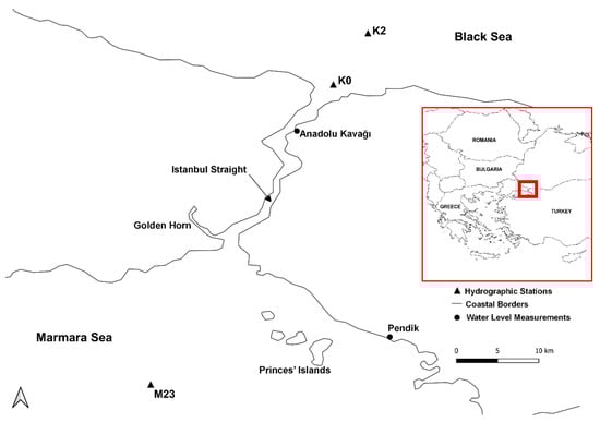
Figure 1.
Study area and hydrographic observation stations in the Istanbul strait [25].
As mentioned above, the most significant feature of the flow in the Istanbul Strait is that there are two different flows in the upper and lower layers in opposite directions. In Figure 2, the longitudinal section of the strait is given with a schematic representation of the flow structure. While the upper layer flow is towards the south, from the Black Sea to the Marmara Sea, the lower layer flow is towards the north, from the Marmara Sea to the Black Sea. Less salty (hence lighter) Black Sea water constitutes the upper layer of the strait. The upper layer is colder than the lower layer in the winter months and warmer in the summer months. The lower layer is saltier than the upper layer, and coming from the Mediterranean Sea [4]. The intermediate (mixing) layer lies between the upper and lower layers, and the thickness of this layer oscillates with the effect of internal waves.
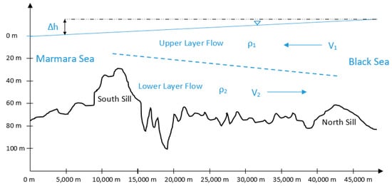
Figure 2.
Schematic description of the longitudinal section of the Istanbul Strait based on [2].
For setting up a reliable numerical model, bathymetric, mareographic, hydrographic, and meteorological data are essential. For the present study, bathymetric data was obtained from the Turkish Navy Office of Navigation, Hydrography, and Oceanography.
The water-level differences between two sides of the strait—which govern the hydrodynamic structure of the flow through the strait—are used as input forcing in the model. For this purpose, mareographic data for 2003 was obtained from the Turkish Naval Forces. The southern and northern boundaries of the strait are represented by the water-level data of the Pendik and Anadolu Kavağı stations, respectively, as shown in Figure 3. The hourly measured water-level data is input in the model, but in Figure 3, the daily averaged data is presented for the sake of keeping the figure visually simple. As it is known, the water level of the Black Sea is higher than the Marmara Sea side over the whole year, except for the cases involving strong southerly blowing winds. The water-level data is consistent with this fact, and is thus seen to be reliable.
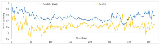
Figure 3.
Daily water-level values in the Pendik and Anadolu Kavağı mareography stations in 2003.
As stated above, the main reason for the stratification of the strait is the density variation by depth. Two main factors affecting the density variation, salinity and temperature, are incorporated in the hydrodynamic model. Salinity and temperature variation data were taken from the ISKI (Istanbul Water and Sewerage Administration) hydrographic observation stations [25]. Stations K0 and K2 are selected for the northern boundary, whereas station M23 is chosen for the southern boundary, which are shown in Figure 1. For two boundaries of the strait, monthly observations of the salinity and temperature data are used as an input parameter in the model (Figure 4). As seen in Figure 4, salinity and temperature data are measured monthly, and they generally reflect the stratification in the strait. It can be seen apparently in the temperature data that a cold intermediate layer is prominent in the months between May and September, as mentioned before.
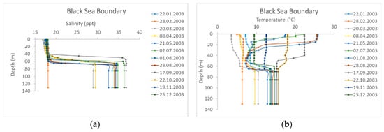
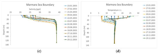
Figure 4.
The first row shows (a) the salinity and (b) temperature of the Black Sea boundaries of the Istanbul Strait; and the second row shows (c) the salinity and (d) temperature of the Marmara Sea boundaries of the Istanbul Strait.
For modeling the hydrodynamical structure of the Istanbul Strait, meteorological data is required to include the effect of atmosphere–sea interaction taking place at the near-surface part of the water mass, since wind shear and barometric differences are important flow forcing factors, as well as the water-level and density differences. To serve as input data for the model, mean sea-level pressure values, and wind velocity components u (east–west direction) and v (north–south direction) at 10-m altitude are obtained from European Centre for Medium-Range Weather Forecasts (ECMWF) database.
Model Setup
The hydrodynamic model of the Istanbul Strait is established in Delft3D-FLOW. This model is based on the finite element method, and is often used in the hydrodynamical modeling of coasts, rivers, estuaries, and seas, with governing equations of fluid dynamics [35]. These equations are the Navier–Stokes equations, which also includes Reynolds stresses (RANS equations) with the k-ε closure. It should be noted that Delft3D-FLOW operates with hydrostatic pressure instead of solving the whole suit of RANS equations. Details can be found in [35].
To set up the hydrodynamic model in Delft3D-FLOW, the following steps are applied: (1) computational grid generation, (2) an input of bathymetric conditions, (3) the input of other parameter values, (4) an initial conditions assignment, (5) a boundary conditions assignment, and (6) selection of the observation point locations (locations for model output).
To simulate fluid motions, continuity and momentum equations (RANS equations) should be solved. However, these equations—especially momentum equations—are in the form of non-linear partial differential equations. Since these equations are non-linear, it is not possible to solve them analytically. The numerical finite difference method is used to approach the exact solution of these equations in a computationally efficient manner. The computational grid, which is an important part of the solution scheme, was generated by discretizing the flow domain using the RGFGRID module of Delft3D. In the model, horizontal and vertical grids were used. The horizontal grid facilitates the representation of the fluid motions throughout the strait in the north–south direction (Figure 5a). The Horizontal Grid domain used in the model covers the region between 30.0354–28.0944 longitudes and 41.4756–40.7878 latitudes. The total horizontal grid cell quantity is 685. The maximum and minimum grid lengths are 6161 m and 198 m, respectively. The coarse (≈6000 m) section of the computational grid corresponds to open sea zones. The grid spacing gets finer inside of the Istanbul Strait for maintaining the computational efficiency as well as computational accuracy.
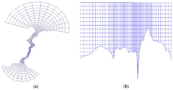
Figure 5.
Hydrodynamic grid of the model in the (a) vertical and (b) horizontal directions.
The vertical grid is also important to observe the stratification effect. Unlike many previous research studies [36,37,38], a z-model was used in this study in favor of a σ-model, meaning that the number of grid cells in the vertical were not constant, but rather variable as a function of depth. This is because the z-model is known to be more capable to accurately model stratified flow conditions [35]. As shown in Figure 5b, the vertical grid lines are perpendicular. Nevertheless, the perpendicularity of grids is distorted occasionally, especially in the near-bottom regions. However, in the Intermediate Layer, the perpendicularity is intact and avails stratification of the flow field. All vertical grid lengths are taken as constant at 5 m.
The bottom topography of the strait exhibits an irregular and variable shape. Figure 6 shows the point-based (raw data) and refined area based bathymetry. Refined bathymetry is established in the QUICKIN module of Delft3D by the triangular interpolation method. This way, a more realistic bathymetric boundary condition can be achieved.
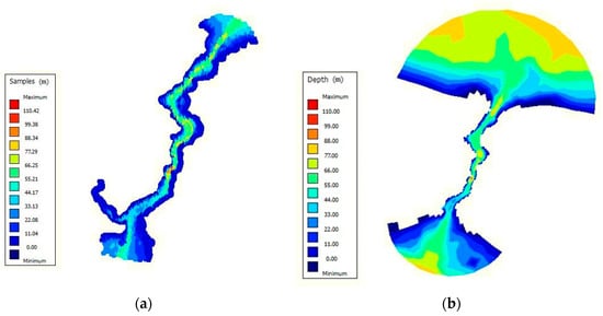
Figure 6.
Point-based (raw) (a) and area-based (refined) bathymetry data of the strait (b).
There are several other input parameters in the model such as time-related parameters, roughness, viscosity, and turbulence parameters. Time-related parameters include the time domain and time step parameters. The time domain of the numerical run starts on 1 January 2003 at 00:00:00 and finishes on 1 January 2004 at 00:00:00. The time step of 0.25 min (15 s) was chosen, as it was small enough to accurately capture the unsteady behavior of the flow. Five of the input parameters: (1) Manning roughness coefficient, (2) horizontal eddy viscosity, (3) slope in log–log spectrum, (4) Prandtl–Schmidt number, and (5) spatial low-pass filter—are designated as calibration parameters. The vertical eddy viscosity and diffusivity parameters are 10−4 m2/s and 10–5 m2/s [35]. As mentioned above, the k- turbulence model is selected in the model.
Water-level values at both ends of the strait were chosen for the hydrodynamic open-boundary conditions. As mentioned above, as the northern boundary conditions, we dictated Anadolu Kavağı water-level data (Figure 3) to the model as input, and for the southern boundary conditions, we dictated Pendik water-level data (also in Figure 3) to the model as input.
For the transport boundary conditions, hydrographic (salinity and temperature) data were used. For northern boundary conditions, the data given in Figure 4a,b were used, whereas the data presented in Figure 4c,d were adopted for southern boundary conditions.
The initial conditions values of four model parameters needed to be defined, which were: water level, velocity, salinity, and temperature. In the model, the initial water level and velocity values were assumed as 0, termed as "Cold Start". This means that the boundary conditions will determine the flow structure of the model substantially. As salinity and temperature, the average values of Figure 4 were adopted. For instance, the average values of Figure 4a,c, give us a representative salinity data for the whole domain. In the same way, the mean values of Figure 4b,d, conceive initial temperature values.
In order to calibrate the model by flowrates, two different techniques were used in addition to the manual calibration: (1) the gradient-based Levenberg–Marquardt method [39,40,41], and (2) the covariance matrix adaptation evolution strategy (CMA-ES) [42,43]. The Levenberg–Marquardt (LM) method finds the local best solution, whereas CMA-ES is a global metaheuristic search algorithm. Although there is another well-known method available in PEST toolbox i.e., the shuffled complex evolutionary algorithm [44], we chose CMA-ES, as it usually converges faster. There are many more methods in the optimization literature such as the genetic algorithm, Dynamically Dimensioned Search (DDS) etc.; however, we focused on only these two methods to limit our experiments within the time limit of this Special Issue. We used two metrics—(1) SPAtial EFficiency (SPAEF) [45] and the (2) correlation coefficient (CORR)—to evaluate the temperature and salinity profiles simulated by the model.
3. Results
Before the calibration process, the most sensitive parameters that affect the model results are determined using the one-at-a-time local sensitivity analysis method based on the Jacobian matrix in the PEST toolbox [39]. Initially, the number of calibration parameter candidates was 17. These parameters are the Manning roughness coefficient; horizontal and vertical eddy viscosities; horizontal and vertical eddy diffusivities; wind stress coefficients A, B and C; wind speed coefficients A, B and C; Secchi depth; Stanton and Dalton numbers; slope in log–log turbulence spectrum; Prandt–-Schmidt number; and spatial low-pass filter coefficient. The relative sensitivity values of these parameters, as evaluated by the Levenberg–Marquardt method, are given in Table 1. According to this sensitivity analysis, the spatial low-pass filter coefficient, horizontal eddy viscosity, Prandtl–Schmidt number, slope in log–log spectrum, and Manning roughness coefficient are the parameters for which the model results have the highest sensitivity. Therefore, these five parameters were selected for the model calibration using the LM and CMA-ES methods.

Table 1.
Sensitivity analysis results using the Levenberg–Marquardt algorithm (PEST) tool [41,46]
After the sensitivity analysis, the important parameters were selected and calibrated, as shown in Table 2.
Table 2.
Calibrated values of the model parameters using three methods. CMA-ES: covariance matrix adaptation evolution strategy, LM: Levenberg–Marquardt.
Table 2 shows that PEST-LM yielded the most realistic value as far as the Manning roughness coefficient is concerned. For the Istanbul Strait, having a non-vegetated naturally formed seabed, a textbook guess for the Manning roughness coefficient would be around 0.025–0.035 [47]. While 0.02 is quite below this expected range, the value calibrated by the PEST-LM method successfully captures this range.
Likewise for the horizontal eddy viscosity, a value around at the order of 10 m2/s is much more realistic than a value around 1 m2/s, considering that the mesh (grid) size adopted in the present study is in the order of hundreds to thousands of meters, and the enhanced resistance due to subgrid turbulence should be accounted for in the horizontal eddy viscosity value.
When it comes to the other calibration parameters given in Table 2, the values achieved by all three methods are not radically different from each other, also are close to the values given in the literature. To sum up, among the three methods employed, PEST-LM proved to yield the most physically consistent values for all the parameters.
The flow rates calculated by the model were extracted as model output in the sections that are located in the northernmost and the southernmost parts of the strait. To test the reliability of the flow rate results of the model, ensemble-averaged monthly mean flow rate measurements for each month from 1999 to 2010 were taken into consideration, as shown in Table 3 [21]. In this table, lower layer flow rate values directed to the north are shown as a negative, while the velocity vectors of southward flow in the upper layer are assumed as positive.
Table 3.
The average of 10 years of in situ flow rate values measured in the north and south of the strait [21].
3.1. Hydrodynamic Model Calibration
In this study, the monthly average flow rate values (from January to December) computed by the numerical model are compared with the ensemble-averaged monthly mean values of the 10 years of in situ observations. Figure 7 and Figure 8 show the modeled and observed monthly average flow rates for the lower and upper layers at the northern and southern parts of the strait.
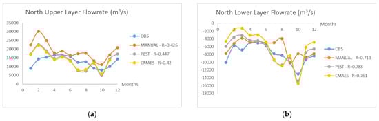
Figure 7.
Upper (a) and lower (b) flow rate values of the northern part of the strait.
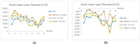
Figure 8.
Upper (a) and lower (b) flow rate values of southern part of the strait.
When Figure 7 and Figure 8 are investigated, it can apparently be seen that the Levenberg–Marquardt calibration algorithm (PEST-LM) is the best-fitting method generally [39]. Especially in the northern part of the strait, the agreement of the PEST-calibrated model output with the observed values is remarkable. On the other hand, the PEST-LM method cannot be said to be the most efficient method for calibration. When it comes to the south station measurements, manual calibration and CMA-ES performed slightly better than the PEST-LM method.
According to Figure 7 and Figure 8, it is understood that observations and modeled flow rates are generally in accordance. One can easily see that the north and south flow rates are not the same. This difference between flow rates originates from the mixing taking place between the lower and upper flow layers. For instance, a water element traveling from the Marmara Sea through the lower layer northwards tends to entrain to the upper layer in the “hydraulic control” sections. As mentioned before, these sections are the locations of the most significant vertical mixing flows in the strait. This mass transfer between the two layers introduces the differences between flow rates recorded at the north and south sections.
Altiok et al. [26] mentioned two extreme conditions in 2003, which are seen in Figure 7 and Figure 8. According to the research, the upper layer flow rate increased uncommonly because of the augmentation in Danube River discharge during that year. The Danube River is the most effectual stream for the Black Sea, which impacts the strait’s upper layer flow rate. The other extreme event is the extraordinary increment in the lower layer flow rate in October, which was due to the anticyclonic eddies in the northern side of the strait. The results of the proposed model seem to capture both of these exceptional events, so it could be said that the flow rate values can be estimated with a fair consistency.
3.2. Hydrographic Model Validation
As mentioned above, the model is calibrated according to monthly average flow rate values. Although the performance of the calibration process was shown to be satisfactory, calibration alone is not always sufficient to prove the reliability of the model. To validate the model in a robust way, the salinity and temperature process profiles along the strait are also examined. Figure 9 presents the longitudinal salinity profiles of the Istanbul Strait for four different months, namely January, April, July, and October. According to this figure, the dispersion and distribution of salinity in the model substantially agrees with the in situ observations. Stratification in the strait clearly reveals itself in salinity profiles, such that the upper and lower flow layers can easily be distinguished. Normally, the upper zones are less saline, around 18–20 ppt, and the deeper zones are more saline, around 38–40 ppt. This is because the upper layer originates from Black Sea, and is thus fed by less saline sources such as the Danube River, while the source of the lower layer is the saline waters of Marmara, Aegean, and Mediterranean seas. It can be seen from the model results as well as observations that when the flow rate of the upper layer increases, the thickness of this layer with the less saline water mass (blue in the figures) also increases.
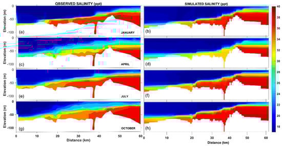
Figure 9.
Salinity profiles observed (a) and modeled (b) in January, observed (c) and modeled (d) in April, observed (e) and modeled (f) in July, and observed (g) and modeled (h) in October.
Another conspicuous feature of the strait is the variation in seawater temperature in the vertical measurements. Figure 10 gives the longitudinal temperature profiles of the strait, respectively in January, April, July, and October. This figure also involves the model results as well as the measured temperature profiles. The most imperative feature of the strait, stratification, is also clearly represented by the numerical model from the temperature viewpoint. Although a general agreement between the model results and the measured data can be assessed, it is seen that the performance of the numerical model for modeling the temperature profiles is not as effective as salinity modeling. The potential reason is that more complicated atmospheric effects (such as atmospheric cooling and warming) are engaged in the temperature modeling, and this is in contrast to the salinity, which is mostly governed by the oceanographic/mareographic parameters. Nevertheless, it can generally be said that the profiles of the stratified temperature structure were captured by the numerical model results, even though it is not as accurate as the salinity profiles. For instance, in January and April, the upper layer is colder than the lower layer, and in July and October, vice versa. Both conditions are exhibited in the numerical model within a fair approximation. A visible drawback in the model is that the thickness of the intermediate layer could not always be properly modeled. Especially in the July results, this defect is observed. Irrespective of the drawback, it can be said that the observed temperature profiles are modeled with a fair agreement. Along with the agreement of the model results and measurements, the salinity and temperature profiles are also accord with recent studies such as those of Sözer and Özsoy [30], Sannino et al. [31], and Aydoğdu et al. [48]. Although these studies do not include modeling seasonal variations of salinity and temperature profiles, results regarding the stratification and density gradient phenomena are generally overlapping with the present study. Considering that only a few studies have included seasonal hydrographical modeling [49,50], modeling the hydrographical features of the strait in various seasons may be recorded as a novelty of this study. Based on the SPAEF results in Table 4, the fit between monthly observed and simulated salinity profiles are reasonable. Only the summer temperature performance of the model revealed low SPAEF (−0.45) and CORR (−0.04) values that are both below zero. The main reason for this poor fit is thought to be that modeling the wintry cold intermediate layer is quite complicated. When the atmospheric temperature rises, the upper layer of the strait gets warm. As a result, the residual winter cold water mass in the upper layer settles between the warm upper layer and the cooler lower layer. Conceivably, this involved phenomenon could not be modeled properly.
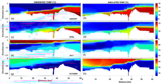
Figure 10.
Temperature profiles observed (a) and modeled (b) in January, observed (c) and modeled (d) in April, observed (e) and modeled (f) in July, and observed (g) and modeled (h) in October.
Table 4.
Visual performance of the model.
4. Discussion
In this study, the Istanbul Strait, one of the most complicated waterways in the world with its meandering shape, stratified structure, and hydraulic control process, was numerically modeled. The main objective of the study is to model the hydrodynamic and hydrographic constitution of the strait, as well as assess the most sensitive hydrodynamic parameters to reach a successful solution.
Three different methods were employed for calibration of the model by comparing the in situ measured flow rates of the upper and lower layers of the north and south parts of the strait with the numerical model results. Among the employed methods, the Levenberg–Marquardt algorithm (PEST method) came out to be the best to calibrate the model, not only due to the closest agreement between the measurements and the model, but also with the physically consistent values of the input parameters attained as the end product of the calibration process. With the mentioned method used, the correlation between numerical model results and observations got higher. Especially in the northern section of the strait, the method was perceptibly successful.
Sensitivity analysis showed that among the 17 input parameters, the following five had the most prominent effect on the results: (1) spatial low-pass filter coefficient, (2) horizontal eddy viscosity, (3) Prandtl–Schmidt number, (4) slope in log–log spectrum, and (5) Manning roughness coefficient.
Apart from the flow rate results of the upper and lower layers, we used the numerical model to assess the salinity and temperature profiles of the stratified flow in the strait, in comparison with the in situ measurements. This latter comparison served as a means of validating the numerical model. The modeled salinity profiles came out to be another prosperous output of this study. Besides the stratification of the strait, the salinity values and layer thicknesses were modeled in good agreement with the measurements, such that the modeled and observed salinity profiles closely resembled each other. When it comes to the temperature profiles, stratification and seasonal variations were seen as fairly represented in the numerical model results. Although the thickness of the intermediate cold layer was not accurately estimated by the model results, the general temperature profiles of the model were seen to be in accord with the observed profiles. Choosing calibration and validation datasets that are very different from each other is one of the unique feature of our study. Obviously, if the calibration framework includes the observed temperature as part of the objective function, the model simulation performance of temperature profiles will substantially increase. This is an ongoing modeling effort, and will be the topic of a subsequent study.
With this numerical modeling study, it was clearly seen that the robustness of the model depends on the sufficient representation of the boundary and initial conditions, as well as the accurate water-level inputs, which are the main forcing factor of the flow. Stratification phenomena can only be modeled through properly assigning the stratified boundary and initial conditions, as was done in the present study.
In future studies, the temporal and spatial domains of the model could be extended in order to model the strait in a more proper way, preferably with a higher grid resolution. As such, the agreement of hydrodynamic and hydrographic outputs between model and the observations could improve in these future studies, and possibly model estimations of the effect of climate change on the delicate flow regime of the Istanbul Strait.
Author Contributions
Conceptualization, M.M.K. and M.C.D.; methodology, M.M.K. and M.C.D.; software, M.M.K. and M.C.D.; validation, M.M.K., M.C.D. and V.S.O.K.; formal analysis, M.C.D. and V.S.O.K.; investigation, M.M.K. and V.S.O.K.; resources, M.M.K. and V.S.O.K.; data curation, M.M.K. and M.O.; writing—original draft preparation, M.M.K., M.C.D., V.S.O.K and M.O.; writing—review and editing, M.C.D. and V.S.O.K.; visualization, M.M.K., M.C.D. and V.S.O.K.; supervision, M.O.
Funding
This research was funded by Istanbul Technical University, grant number 38420. The second author (MCD) is supported by Turkish Scientific and Technical Research Council (TÜBİTAK grant 118C020)
Conflicts of Interest
The authors declare no conflict of interest.
References
- Çeçen, K.; Bayazıt, M.; Sümer, M.; Güçlüer, Ş.; Doğusal, M.; Yüce, H. İstanbul Boğazı’nın Hidrolik ve Oşinografik Etüdü (The Hydraulic and Oceanographic Survey of Istanbul Strait); Istanbul Technical University: Istanbul, Turkey, 1981. [Google Scholar]
- Bayazıt, M.; Sümer, M. İstanbul Boğazı’nın Hidrolik ve Oşinografik Etüdü-2 (The Hydraulic and Oceanographic Survey of Istanbul Strait-2). TBTAK Su. Alma. Ünitesi. Kesin. Rapor. 1982, 23. [Google Scholar]
- Sumer, B.M.; Bakioglu, M. Sea-Strait Flow With Special Reference To Bosphorus; Technical Report; Istanbul Technical University-Civil Engineering Faculty: Istanbul, Turkey, 1981. [Google Scholar]
- Latif, M.A.; Özsoy, E.; Oguz, T.; Ünlüata, Ü. Observations of the Mediterranean inflow into the Black Sea. Deep Sea Res. Part A Oceanogr. Res. Pap. 1991, 38, S711–S723. [Google Scholar] [CrossRef]
- Özsoy, E.; Beşiktepe, Ş.; Latif, M.A. Türk Boğazlar Sistemi’nin Oşinografisi (Oceanography of the Turkish Strait System). In Marmara Denizi 2000 Sempozyumu; Türk Deniz Araştırmaları Vakfı: İstanbul, Turkey, 2000. [Google Scholar]
- Falina, A.; Sarafanov, A.; Özsoy, E.; Utku Turunçoğlu, U. Observed basin-wide propagation of Mediterranean water in the Black Sea. J. Geophys. Res. Ocean. 2017, 122, 3141–3151. [Google Scholar] [CrossRef]
- Sur, H.I.; Özsoy, E.; Ünlüata, Ü. Boundary current instabilities, upwelling, shelf mixing and eutrophication processes in the Black Sea. Prog. Oceanogr. 1994, 33, 249–302. [Google Scholar] [CrossRef]
- Oguz, T.; Özsoy, E.; Latif, M.A.; Sur, H.I.; Ünlüata, Ü. Modeling of hydraulically controlled exchange flow in the Bosphorus Strait. J. Phys. Oceanogr. 1990, 20, 945–965. [Google Scholar] [CrossRef]
- Farmer, D.M.; Armi, L. Maximal two-layer exchange over a sill and through the combination of a sill and contraction with barotropic flow. J. Fluid Mech. 1986, 164, 53–76. [Google Scholar] [CrossRef]
- Armi, L.; Farmer, D.M. Maximal two-layer exchange through a contraction with barotropic net flow. J. Fluid Mech. 1986, 164, 27–51. [Google Scholar] [CrossRef]
- Armi, L. The hydraulics of two layers with different densities. J. Fluid Mech. 1986, 163, 27–58. [Google Scholar] [CrossRef]
- Dorrell, R.M.; Peakall, J.; Sumner, E.J.; Parsons, D.R.; Darby, S.E.; Wynn, R.B.; Özsoy, E.; Tezcan, D. Flow dynamics and mixing processes in hydraulic jump arrays: Implications for channel-lobe transition zones. Mar. Geol. 2016, 381, 181–193. [Google Scholar] [CrossRef]
- Beşiktepe, Ş.T.; Sur, H.I.; Özsoy, E.; Latif, M.A.; Oǧuz, T.; Ünlüata, Ü. The circulation and hydrography of the Marmara Sea. Prog. Oceanogr. 1994, 34, 285–334. [Google Scholar] [CrossRef]
- Özsoy, E.; Latif, M.A.; Besiktepe, S.; Çetin, N.; Gregg, M.C.; Belokopytov, V.; Goryachkin, Y.; Diaconu, V. The Bosporus Strait: Exchange Fluxes, Currents and Sea-Level Changes. NATO Sci. Ser. 2 Environ. Secur. 1998, 47, 1–28. [Google Scholar]
- Gregg, M.C.; Özsoy, E.; Latif, M.A. Quasi-steady exchange flow in the Bosphorus. Geophys. Res. Lett. 1999, 26, 83–86. [Google Scholar] [CrossRef]
- Gregg, M.C.; Özsoy, E. Flow, water mass changes, and hydraulics in the Bosphorus. J. Geophys. Res. 2002, 107. [Google Scholar] [CrossRef]
- Güler, I.; Yüksel, Y.; Yalçiner, A.C.; Çevik, E.; Ingerslev, C. Measurement and evaluation of the hydrodynamics and secondary currents in and near a strait connecting large water bodies-A field study. Ocean Eng. 2006, 33, 1718–1748. [Google Scholar] [CrossRef]
- Yuksel, Y.; Ayat, B.; Özturk, M.N.; Aydogan, B.; Guler, I.; Cevik, E.O.; Yalçiner, A.C. Responses of the stratified flows to their driving conditions-A field study. Ocean Eng. 2008, 35, 1304–1321. [Google Scholar] [CrossRef]
- Aydoǧan, B.; Ayat, B.; Özturk, M.N.; Özkan Çevik, E.; Yüksel, Y. Current velocity forecasting in straits with artificial neural networks, a case study: Strait of Istanbul. Ocean Eng. 2010, 37, 443–453. [Google Scholar] [CrossRef]
- Jarosz, E.; Teague, W.J.; Book, J.W.; Beşiktepe, Ş. Observed volume fluxes in the Bosphorus Strait. Geophys. Res. Lett. 2011, 38. [Google Scholar] [CrossRef]
- Altiok, H.; Kayişoğlu, M. Seasonal and interannual variability of water exchange in the Strait of Istanbul. Mediterr. Mar. Sci. 2015, 16, 644–655. [Google Scholar] [CrossRef]
- Özsoy, E.; Cagatay, M.N.; Balkis, N.; Balkis, N.; Ozturk, B. The Sea of Marmara; Marine Biodiversity, Fisheries, Conservation and Governance; Turkish Marine Research Foundation (TUDAV) Publication: Istanbul, Turkey, 2016; ISBN 9789758825349. [Google Scholar]
- Çolpan Polat, S.; Tugrul, S. Nutrient and organic carbon exchanges between the Black and Marmara Seas through the Bosphorus Strait. Cont. Shelf Res. 1995, 15, 1115–1132. [Google Scholar] [CrossRef]
- Hubareva, E.; Svetlichny, L.; Kideys, A.; Isinibilir, M. Fate of the Black Sea Acartia clausi and Acartia tonsa (Copepoda) penetrating into the Marmara Sea through the Bosphorus. Estuar. Coast. Shelf Sci. 2008, 76, 131–140. [Google Scholar] [CrossRef]
- Sur, H.İ.; Okuş, E.; Güven, K.; Yüksek, A.; Altiok, H.; Kıratlı, N.; Ünlü, S.; Taş, S.; Aslan Yılmaz, A.; Yılmaz, N.; et al. Water Quality Monitoring: Annual Report (2003); Istanbul University Institute of Marine Sciences and Management: Istanbul, Turkey, 2004. [Google Scholar]
- Altiok, H.; Sur, H.İ.; Yüce, H. Variation of the cold intermediate water in the Black Sea exit of the Strait of Istanbul (Bosphorus) and its transfer through the strait. Oceanologia 2012, 54, 233–254. [Google Scholar] [CrossRef]
- Akay, O. Hydrodynamic Simulation of the Bosphorus. M.Sc. Thesis, Istanbul Technical University, Istanbul, Turkey, 2002. [Google Scholar]
- Öztürk, M.N. İstanbul Boğazı’nın Hidrodinamiği ve Sayısal Modellenmesi (Hydrodynamics of the Istanbul Strait and its Numerical Model). Ph.D. Thesis, Yildiz Technical University, Istanbul, Turkey, 2010. [Google Scholar]
- Sözer, A. Numerical Modeling of the Bosphorus Exchange Flow Dynamics. Ph.D. Thesis, Middle East Technical University, Ankara, Turkey, 2013. [Google Scholar]
- Sözer, A.; Özsoy, E. Modeling of the Bosphorus exchange flow dynamics. Ocean Dyn. 2017, 67, 321–343. [Google Scholar] [CrossRef]
- Sannino, G.; Sözer, A.; Özsoy, E. A high-resolution modelling study of the Turkish Straits System. Ocean Dyn. 2017, 67, 397–432. [Google Scholar] [CrossRef]
- Armi, L.; Farmer, D.M. The Internal Hydraulics of the Strait of Gibraltar and Associated Sills and Narrows. Oceanol. Acta 1985, 8, 37–46. [Google Scholar]
- Bruno, M.; Chioua, J.; Romero, J.; Vázquez, A.; Macías, D.; Dastis, C.; Ramírez-Romero, E.; Echevarria, F.; Reyes, J.; García, C.M. The importance of sub-mesoscale processes for the exchange of properties through the Strait of Gibraltar. Prog. Oceanogr. 2013, 116, 66–79. [Google Scholar] [CrossRef]
- Koşucu, M.M. Three-Dimensional Hydrodynamic Model of the Istanbul Strait. Master’s Thesis, Istanbul Technical University, Istanbul, Turkey, 2016. [Google Scholar]
- Delft3D User Manual Simulation of Multi-dimensional Hydrodynamic Flow and Transport Phenomena, Including Sediments. 2014, p. 684. Available online: https://oss.deltares.nl/documents/183920/185723/Delft3D-FLOW_User_Manual.pdf (accessed on 18 September 2019).
- Cornelissen, S. Numerical Modelling of Stratified Flows Comparison of the σ and z Coordinate Systems. Master’s Thesis, Delft University of Technology, Delft, The Netherlands, 2004. [Google Scholar]
- Lesser, G.R.; Roelvink, J.A.; van Kester, J.A.T.M.; Stelling, G.S. Development and validation of a three-dimensional morphological model. Coast. Eng. 2004, 51, 883–915. [Google Scholar] [CrossRef]
- Huang, W.; Spaulding, M. Modeling horizontal diffusion with sigma coordinate system. J. Hydraul. Eng. 1996, 122, 349–356. [Google Scholar] [CrossRef]
- Doherty, J. PEST: Model Independent Parameter Estimation. Fifth Edition of User Manual; Watermark Numerical Computing: Brisbane, Australia, 2005. [Google Scholar]
- Doherty, J. Calibration and Uncertainty Analysis for Complex Environmental Models. Groundwater 2015, 53, 673–674. [Google Scholar]
- Doherty, J. Model-Independent Parameter Estimation(Part I), 6th ed.; Watermark Numerical Computing: Corinda, Australia, 2016. [Google Scholar]
- Hansen, N.; Ostermeier, A. Completely derandomized self-adaptation in evolution strategies. Evol. Comput. 2001, 9, 159–195. [Google Scholar] [CrossRef] [PubMed]
- Hansen, N.; Ostermeier, A. Adapting arbitrary normal mutation distributions in evolution strategies: The covariance matrix adaptation. In Proceedings of the IEEE international conference on evolutionary computation, Nagoya, Tokyo, 20–22 May 1996; pp. 312–317. [Google Scholar]
- Duan, Q.; Sorooshian, S.; Gupta, V. Effective and efficient global optimization for conceptual rainfall-runoff models. Water Resour. Res. 1992, 28, 1015–1031. [Google Scholar] [CrossRef]
- Demirel, M.C.; Mai, J.; Mendiguren, G.; Koch, J.; Samaniego, L.; Stisen, S. Combining satellite data and appropriate objective functions for improved spatial pattern performance of a distributed hydrologic model. Hydrol. Earth Syst. Sci. 2018, 22, 1299–1315. [Google Scholar] [CrossRef]
- Dahlstrom, D.J. Calibration and Uncertainty Analysis for Complex Environmental Models; Watermark Numerical Computing: Brisbane, Australia, 2015; ISBN 978-0-9943786-0-6. [Google Scholar]
- Dey, S. Fluvial Hyrodynamics: Hydrodynamic and Sediment Transport Phenomena; Springer: Berlin, Germany, 2014; ISBN 978-3-642-19061-2. [Google Scholar]
- Aydoǧdu, A.; Pinardi, N.; Özsoy, E.; Danabasoglu, G.; Gürses, Ö.; Karspeck, A. Circulation of the Turkish Straits System under interannual atmospheric forcing. Ocean Sci. 2018, 14, 999–1019. [Google Scholar] [CrossRef]
- Ferrarin, C.; Umgiesser, G. Hydrodynamic modeling of a coastal lagoon: The Cabras lagoon in Sardinia, Italy. Ecol. Modell. 2005, 188, 340–357. [Google Scholar] [CrossRef]
- Lazure, P.; Garnier, V.; Dumas, F.; Herry, C.; Chifflet, M. Development of a hydrodynamic model of the Bay of Biscay. Validation of hydrology. Cont. Shelf Res. 2009, 29, 985–997. [Google Scholar] [CrossRef]
© 2019 by the authors. Licensee MDPI, Basel, Switzerland. This article is an open access article distributed under the terms and conditions of the Creative Commons Attribution (CC BY) license (http://creativecommons.org/licenses/by/4.0/).