
Numerical Calculation and 3-D Imaging of the Arrhenius Temperature Integral


1
The State Key Laboratory of Refractories and Metallurgy, Wuhan University of Science and Technology, Wuhan 430081, China
2
School of Chemical Engineering, University of New South Wales, Sydney, NSW 2052, Australia
3
Key Laboratory for Ferrous Metallurgy and Resources Utilization of Ministry of Education, Wuhan University of Science and Technology, Wuhan 430081, China
*
Author to whom correspondence should be addressed.
Separations 2023, 10(9), 480; https://doi.org/10.3390/separations10090480
Submission received: 28 July 2023
/
Revised: 23 August 2023
/
Accepted: 30 August 2023
/
Published: 31 August 2023
(This article belongs to the Special Issue Research Progress in Separation and Extraction of Ferrous and Non-ferrous Metals)
Abstract
:The Arrhenius temperature integral is typically used in non-isothermal kinetic analysis, which is widely applied in gas–solid reactions in separation processes. In previous studies, researchers provided various methods to solve the temperature integral, but the error usually became significant when the value of x (x = Ea/RT) was too large or too small. In this paper, we present a new series method and design a computer program to calculate the temperature integral. According to the precise calculation of the temperature integral, we first reveal the relationship among the integral, the temperature, and the activation energy, and we find an interesting phenomenon in which the 3-D image of the temperature integral is of self-similarity according to fractal theory. The work is useful for mechanism and theoretical studies of non-isothermal kinetics.
1. Introduction
Non-isothermal chemical kinetics are very important for gas–solid reactions in separation processes. As a result, they have been extensively introduced in disciplines, such as chemical engineering [1,2], mineral technology [3], metallurgical engineering [4], materials science [5], biomass energy [6,7], etc. The reaction rate of a solid-involved reaction is now generally accepted to be
where α denotes the conversion ratio of the concerned substance at time t, f(α) is the mechanism function, and k is the rate constant expressed by the Arrhenius equation:
where A, T, and Ea are the pre-exponential factor, temperature, and activation energy of the reaction, respectively.
For a linear heating process, the heating rate β is usually a function of time,
Combining all of the above equations, re-arranging them, and integrating Equation (1), we obtain
where T0 represents the initial reaction temperature and is set at 298 K in this study, and the initial reaction extent α0 usually equals zero.
The Arrhenius temperature integral is also known as the integral of Boltzmann factor Ψ(T), which is derived from Equation (4),
where another variable x could be introduced as
Then, the temperature integral could be calculated as
where the upper limit of Equation (7) is usually considered to be ∞ regarding T0 in the denominator, which is equal to 0.
Then, the expression of the temperature integral as shown in Equation (7) is extensively regarded as the most concise and the best one for calculation.
The solution of the temperature integral is usually the basic demand for a non-isothermal kinetic study [8]. However, it cannot be analytically solved. With the solution of the temperature integral, constant activation energy and the corresponding kinetic mechanism could be determined in model-based (single-step) reactions, and variable activation energies could be calculated in model-free iso-conversional (multi-step) reactions.
The model-based non-isothermal analysis was dominant for a long time because of its ability to determine the kinetic triplet (pre-exponential factor, activation energy, and reaction model) [9,10]. However, these methods suffer from several problems, among which is their inability to uniquely determine the reaction model. This issue led to the decline of these methods in favor over the latest two decades of iso-conversional methods that evaluate kinetics without model assumptions [11]. Regardless of the kind of method, the evaluation of the temperature integral is an inevitable issue. As a result, there is a bottleneck in kinetic analysis, namely the calculation of the temperature integral.
The temperature integral was first encountered by scientists in the early thermogravimetric analyses [9,10,11,12,13]. Reich and Levi [14] made mistakes since they did not recognize that it is a transcendental function. Although different efforts have been made to solve this puzzle over the past six decades [15,16,17,18,19,20,21,22,23,24,25,26,27,28], troubles still occasionally arise since ‘there is no true value for the integral’, as stated by Tang [27]. The temperature integral has been playing an ‘enigmatic’ role in non-isothermal kinetic analysis. That is, it has appeared to be a necessary evil to be addressed [25].
Flynn [25] and Órfão [17] provided excellent reviews of the temperature integral. According to Flynn’s categorization, these solutions of the temperature integral are classified into three categories: series solutions, complex approximations [29,30], and simple approximations. It is given accurately for x greater than 2 by the rational fraction expression. Truncating the number of terms in the fraction expression, we can obtain one, two, three, and four “rational approximations”. Other series solutions, such as Schlömilch expansion, Bernouli number expansion, and Asymptotic expansion, are all available for the calculation limitation of x in different ranges [13,25].
In model-based non-isothermal analysis, simple and complex approximations were preferred and truncated from those series solutions because the truncated solutions could give the temperature integral an analytical expression and make the whole non-isothermal kinetics analytically solvable. For example, truncating the two-term asymptotic approximation, we can obtain the famous linear plot of ln(g(α)/T2) against 1/T, resulting in a slope of Ea/R. In the other words, it is exactly the famous Coats–Redfern method [12]. In addition to the truncations, some modified approximations were also proposed to improve the calculation precision [8,17,18,19,20,26,27,28].
The numerical calculation of the temperature integral is usually carried out by series methods, and model-free iso-conversional non-isothermal kinetics are usually required. Although the precision of the numerical calculation is better today, there are still backward calculations because of the limitations of the series method itself. Numerical calculation based on the quadrature method was occasionally mentioned in previous papers [24,28]. However, the residual error usually increases with the rise in the upper limit temperature of the integration, or it increases with the decrease in x [25]. As a disquieting situation, some published papers provided the wrong quadrature results as standard integral values, such as in Ref. [24].
There were hundreds of papers focused on the solution of the temperature integral once it was suggested that a relative error of 10% for the temperature integral could be acceptable for many calculations. However, more accurate values are still necessary for scientific purposes, such as distinguishing between reaction mechanisms [25]. Furthermore, a more accurate solution possible today with computer technology. All in all, accurate values and numerical calculation methods of the temperature integral are always attractive in non-isothermal kinetic analysis.
2. Theory
So far, most of the solutions for the temperature integral have been based on the concise Equation (7). However, the upper limit of the integration may be far from ∞, resulting in the corresponding inaccurate mathematical equations of series methods.
At the same time, all approximations of the temperature integral take a detour; errors and troubles cannot be eradicated. The only way to obtain the exact numerical solution of the integral is to develop an appropriate series solution, which easily reaches convergence. Here, we provide a new series solution based on Taylor’s expansion:
where ΔT is the difference between T and T0, T = T0 + ΔT, and n denotes the order of Taylor expansion.
Then, the exact derivative value at temperature T0 could be calculated using Equations (7)–(9).
The n-th-order derivative expression shown as Equation (9) is established according to Leibniz formula [31]. With the help of the general form of the n-th-order derivative equation, we designed a computer program to calculate the integral of the Boltzmann factor with Equation (6). The numerical value can converge within a sufficiently small residual error when the derivative order n is large enough, and ΔT is small enough. Computing the results shows that the value usually converges with reasonably little error when n is greater than 4 and ΔT is no greater than 50 K. Consequently, a multi-step integral method is applied to compute the integral value when the difference between the upper and lower limit temperature is larger than 50 K. The corresponding error analysis of the present calculation method is also provided below.
3. Error Analysis
Table 1 shows the converging evolution of the integral value with increasing order of Taylor expansion. Most of the values converge within a relative error of 1‰ when the Taylor order is larger than 4. A relative error within 10−8 can be achieved when the Taylor order increases to 10. To reach high accuracy, a 3D image (Figure 1a) of the integral function is established based on 200 × 200 calculation nodes, and each node is computed with a Taylor order of 20.
As shown in Figure 1a–d, the integral values have differences in orders of magnitude from each other with different temperatures and activation energies. To control computing error, the relative residual was defined as follows:
where Ψ(n, T, Ea) denotes the integral of Boltzmann factor with upper limit temperature of T, activation energy of Ea, and Taylor order of n. The relative residual δ denotes a tolerance when it is presupposed as a maximum limitation that should not be exceeded.
Figure 1a–d demonstrates the minimum required Taylor order for calculating the temperature integral under error tolerances of 10−4, 10−8, 10−12, and 10−16, respectively. According to Figure 1a,b, the relative residual errors in Figure 1a are no greater than 10−4 under the domain of definition, and most of the values have a residual error of 10−8. The smaller that the minimum required Taylor order is, the more easily that the iteration reaches tolerance. In previous studies, it is simply concluded that the errors become significant when the value of x (x = Ea/RT) is too small or too large [25]. However, according to these figures, a different trend is discovered. Generally, the trend that is proved by these four figures is that the minimum required Taylor order rises with a decreasing upper limit or an increase in the activation energy when the upper limit temperature is greater than about 350 K, and the minimum required Taylor order rises with increasing the upper limit or increase in the activation energy when the temperature is between 298 and 350 K.
Furthermore, the relationships among T, Ea, and Taylor order n are more complicated than monotonic, and some singular points also exist in the plots. However, the maximum required Taylor order is no greater than 45 under a tolerance of 10−16, which proves that it is easier to approach convergence than the former methods [25].
Another series solution is established to perform a comparison. Using the Newton–Leibniz quadrature method as a usual idea to resolve it, we obtain:
where
However, we find that the Newton–Leibniz quadrature method was difficult to converge, as shown in Table 2. Moreover, it is not realistic to adopt this method in kinetic analysis because it always requires a massive amount of time to reach high precision. As shown in Table 1, the results converge within 8 accurate digits after the decimal point when the Taylor order n is only larger than 15.
Table 3 provides specific expressions of the commonly used approximate solutions for the temperature integral. The values of temperature integral calculated by MATLAB were used to check the accuracy of other approximation methods. Table 4 reports the temperature integral values calculated by different methods. Except for the present solution, the other values are calculated based on a published article [29], in which the original values are equivalent to Ψ/[T·exp(−Ea/(RT))]. In Table 4, the temperature integral values of the present method and Órfão III’s approximation are fully consistent with MATLAB’s values. Therefore, the new series solution can provide sufficient, accurate values. In contrast, other approximations provide unreliable values when the value of x tends toward minority.
4. Results and Discussion
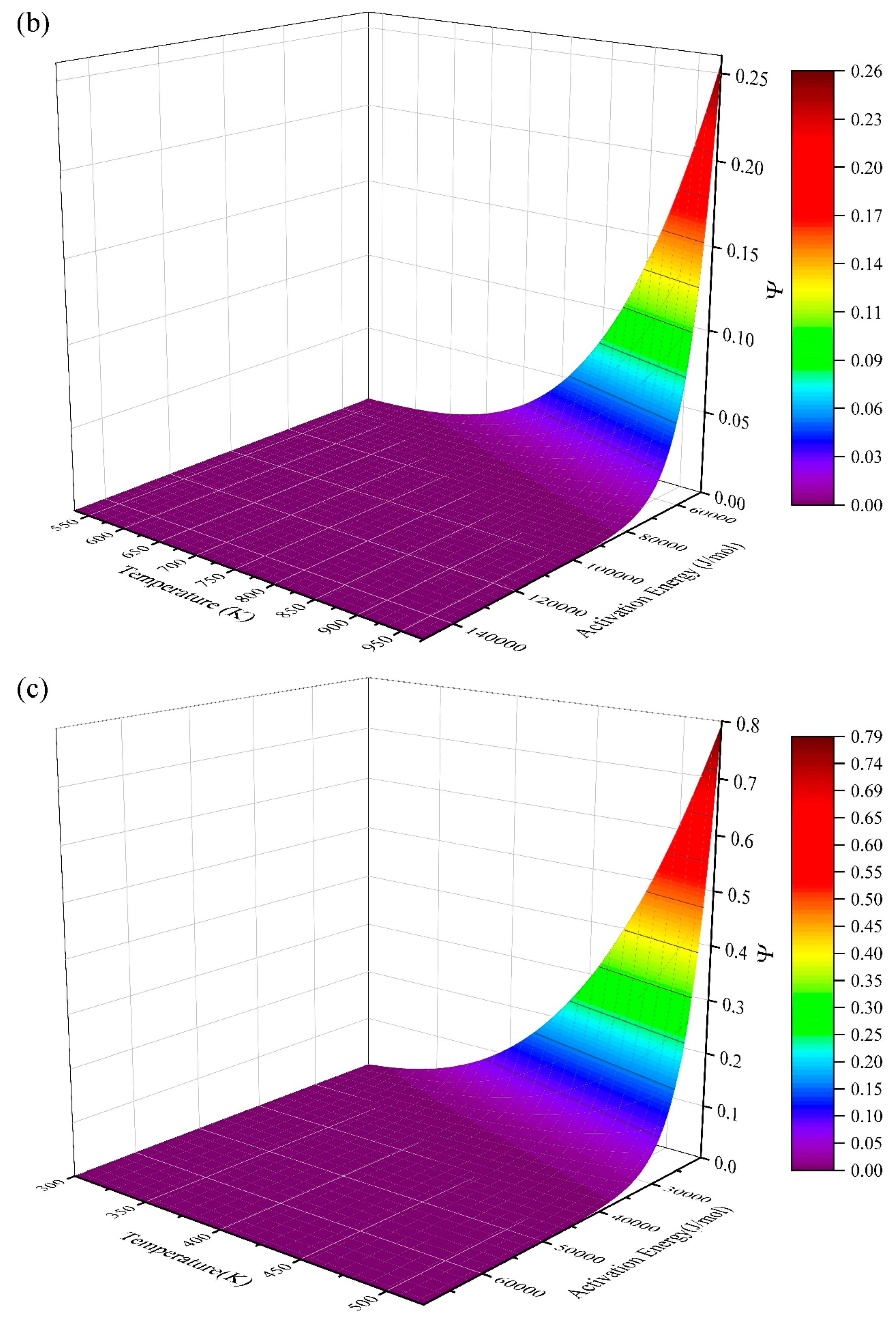
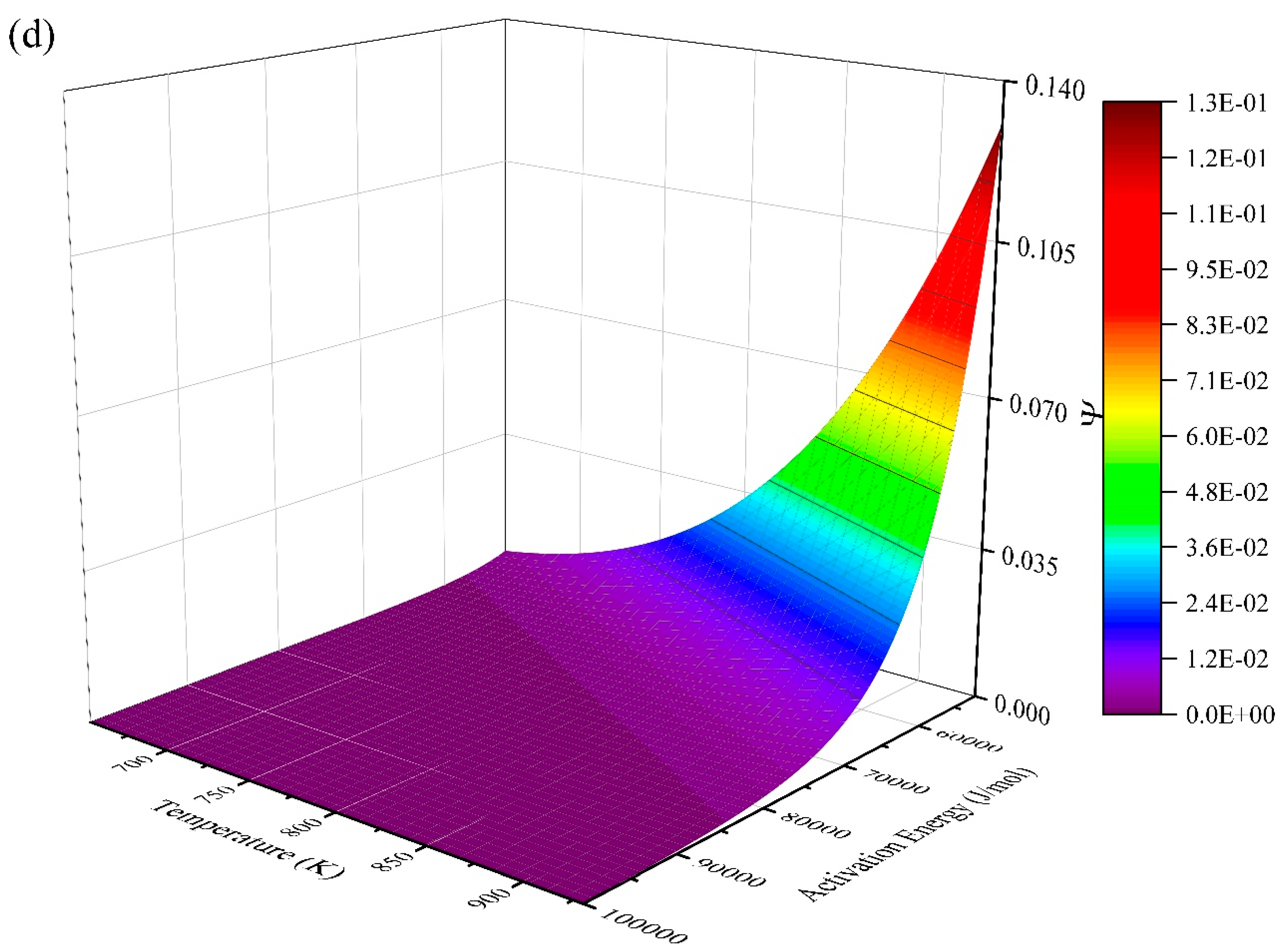
The dependence of the temperature integral on Ea and T has always been a mysterious relationship. Here, we show the true value of the integral in Figure 2a. This image is drawn based on 200 × 200 calculation nodes, and each node is computed with the Taylor order of 20 to ensure the numerical value is accurate enough. It can be seen that the integral value declines by an order of magnitude with the growth of the activation energy, proving that the integral value is extremely sensitive to the activation energy. Therefore, the approximation method often provides an inaccurate value and fails to distinguish the kinetic mechanisms [26]. The integral value tends to be equivalent to the value of ΔT when Ea infinitely approaches 0 kJ/mol, while the integral value declines by an order of magnitude and tends to be 0 when Ea is greater than about 75 kJ/mol.
There is also an interesting phenomenon in that the profile of the 3D surface is relatively similar to others if the independent variables (temperature, activation energy) are arbitrarily truncated, such as in images (b), (c), and (d). Image (a) is drawn based on a 200 × 200 node network, and each node is computed with the Taylor order of 20 to ensure the numerical value is accurate enough. Independent variables Ea and T vary from 2 to 200,002 J/mol and 300 to 1200 K, respectively. In the aforementioned node network (200 × 200), mid nodes (Ea varies from 50,002 to 149,002 J/mol, and T varies from 529.5 to 975 K) are chosen to form a new node network (100 × 100); then, image (b) can be drawn. The node network of image (c) is 50 × 50, and its values of Ea and T change from 20,002 to 69,002 J/mol and from 300 to 520.5 K, respectively. Regarding image (d), its node network is 49 × 63, and corresponding ranges of Ea and T are 52,002 to 100,002 J/mol and 651 to 930 K, respectively. As we can see, the truncated images b, c, and d are similar to the original image a. This phenomenon indicates the self-similarity property of the figure according to fractal theory [38].
5. Conclusions
Because of the demand for accurate solutions related to non-isothermal kinetics, previous researchers have provided various methods to solve the temperature integral, but the error usually becomes significant when the value of x (x = Ea/RT) is too small or too large. A numerical method is proposed to obtain an accurate value of the temperature integral. Multi-step and 20th Taylor expansion are applied to ensure the high accuracy of results calculated by the new method.
The results show that, when the upper limit temperature is greater than about 350 K, the error rises with the decreasing upper limit or the increasing activation energy; when the temperature is between 298 and 350 K, the error rises with the increasing upper limit or the increasing activation energy.
The temperature integral function is very sensitive to the activation energy according to the error analysis and could be well displayed by the 3-D image. The reason why the solution is always divergent when the value of x (x = Ea/RT) is too small or too large, as widely encountered in previous study, can be well interpreted by the contour image of the minimum Taylor order required when using the present method within the iterative tolerances. More interesting, the 3-D image of the temperature integral demonstrates self-similarity according to fractal theory.
6. Resource Codes
Here we share our resource codes for scientific purposes. Anyone who directly uses/translates these codes to produce new papers must cite this paper. All codes below are written in Visual Basic language.
These codes are easily transplanted into a project because they are written in functions. To use these codes, one should first define the environmental temperature (T0, default as 298 K), the presupposed Taylor expansion order (s), the Arrhenius energy (Ea), and the upper limit temperature (T1) of the integral. If the precision worsens, it only requires a smaller iteration temperature (default as 50 K in the code) and a larger Taylor expansion order. Usually, an iteration temperature of 50 K and a Taylor expansion order of 10 are good enough to reach a rational precision.
Option Explicit
Public T0 As Double’ T0 is the initial reaction temperature, default as 298K
Public i As Integer, k As Integer
Public ddg() As Double
Public store() As Double ‘Dynamic array for storage
Public store2() As Double
Public sum As Double
Function Psai(s As Integer, Ea, t1) ‘ Main function: calculation at an arbitrary temperature T1
Dim hun As Integer, jj As Integer
hun = Int((t1 − T0)/50)
ReDim Preserve store2(hun)
Dim sum0 As Double
sum0 = 0
If hun = 0 Then
Psai = gT(s, Ea, t1, T0)
Else
For jj = 1 To hun
store2(jj − 1) = gT(s, Ea, T0 + jj * 50, T0 + (jj − 1) * 50)
sum0 = sum0 + store2(jj − 1)
Next jj
Psai = sum0 + gT(s, Ea, t1, T0 + hun * 50)
End If
End Function
Function Factorial(n) ‘The n-th Factorial
If n = 0 Then
Factorial = 1
Else
Factorial = 1
For i = 1 To n
Factorial = Factorial * i
Next
End If
End Function
Function dg(n As Integer, Ea, T) As Double ‘ n-th derivative of g(T) for successive calculation.
Erase ddg()
ReDim ddg(n) ‘The n-th item in the polynomial expression of n-th-order derivative
ReDim Preserve store(n)
sum = 0
ddg(0) = Exp(−Ea/(8.314 * T))
store(0) = ddg(0)
If n > 0 Then
ddg(1) = Ea * Exp(−Ea/(8.314 * T)) * T ^ −2/8.314
store(1) = ddg(1)
End If
If n = 0 Then
dg = ddg(0)
ElseIf n = 1 Then dg = ddg(1)
Else
Dim m As Integer
m = n − 1
For k = 0 To m Step 1
ddg(k + 1) = (−1) ^ (m − k) * (m + 1 − k) * (Factorial(m)/Factorial(k)) * store(k) * T ^ (k − m − 2)
sum = sum + ddg(k + 1)
Next k
store(n) = sum * Ea/8.314
dg = store(n)
End If
End Function
Function dg_X(n As Integer, Ea, T) ‘ n-th-order derivative of g(T), unconditional
ReDim Preserve store(n)
For i = 0 To n
store(i) = dg(i, Ea, T)
Next i
dg_X = store(n)
End Function
Function gT(n As Integer, Ea, T, T00) ‘ Calculation for temperature difference smaller than 50 K
Dim j As Integer
sum = 0
For j = 1 To n
sum = sum + dg_X(j − 1, Ea, T00) * (T − T00) ^ j/Factorial(j)
Next j
gT = sum
End Function
7. Standard Integral Values
To be compared with the other values of temperature integrals, the standard integral values calculated by the present method are reported in Table 5 below.
Author Contributions
Conceptualization: W.Z.; writing—original draft: W.Z., Q.Z. and K.L.; writing and editing: X.Y. and Y.S. All authors have read and agreed to the published version of the manuscript.
Funding
This research was funded by the Key Technologies R & D Program of Hubei Province, grant number 2022BCA058 and The APC was funded by the same funder.
Data Availability Statement
All data are available by contacting the corresponding author.
Acknowledgments
Many thanks to Chengzhi Li, Juhua Zhang, and Guangqiang Li for their suggestions and to Zhengliang Xue for his support.
Conflicts of Interest
The authors declare no conflict of interest.
References
- Gautam, R.; Vinu, R. Unraveling the interactions in fast co-pyrolysis of microalgae model compounds via pyrolysis-GC/MS and pyrolysis-FTIR techniques. React. Chem. Eng. 2019, 4, 278–297. [Google Scholar] [CrossRef]
- Nestler, F.; Müller, V.P.; Ouda, M.; Hadrich, M.J.; Schaadt, A.; Bajohr, S.; Kolb, T. A novel approach for kinetic measurements in exothermic fixed bed reactors: Advancements in non-isothermal bed conditions demonstrated for methanol synthesis. React. Chem. Eng. 2021, 6, 1092–1107. [Google Scholar] [CrossRef]
- Zhang, J.; Zhang, W.; Xue, Z. Oxidation Kinetics of Vanadium Slag Roasting in the Presence of Calcium Oxide. Miner. Process. Extr. Metall. Rev. 2017, 38, 265–273. [Google Scholar] [CrossRef]
- Wang, H.H.; Li, G.Q.; Yang, J.; Ma, J.; Khan, B.S. The behavior of phosphorus during reduction and carburization of high-phosphorus oolitic hematite with H2 and CH4. Metall. Mater. Trans. B Process Metall. Mater. Process. Sci. 2016, 47, 2571–2581. [Google Scholar] [CrossRef]
- Jiang, Y.H.; Liu, F.; Song, S.J. An extended analytical model for solid-state phase transformation upon continuous heating and cooling processes: Application in γ/α transformation. Acta Mater. 2012, 60, 3815–3829. [Google Scholar] [CrossRef]
- Fermoso, J.; Gil, M.V.; Pevida, C.; Pis, J.J.; Rubiera, F. Kinetic models comparison for non-isothermal steam gasification of coal–biomass blend chars. Chem. Eng. J. 2010, 161, 276–284. [Google Scholar] [CrossRef]
- Tai, H.-C.; Li, G.-C.; Huang, S.-J.; Jhu, C.-R.; Chung, J.-H.; Wang, B.Y.; Hsu, C.-S.; Brandmair, B.; Chung, D.-T.; Chen, H.M.; et al. Chemical distinctions between Stradivari’s maple and modern tonewood. Proc. Natl. Acad. Sci. USA 2017, 114, 27–32. [Google Scholar] [CrossRef]
- Aghili, A. Representation and evaluation of the Arrhenius and general temperature integrals by special functions. Thermochim. Acta 2021, 705, 179034. [Google Scholar] [CrossRef]
- Zhang, W.; Li, K.; Dong, J.H.; Li, C.Z.; Liu, A.H.; Zhang, J.H.; Xue, Z.L. Kinetic triplet from low-temperature carburization and carbon deposition reactions. J. Iron Steel Res. Int. 2022, 29, 1545–1558. [Google Scholar] [CrossRef]
- Li, K.; Zhang, W.; Fu, M.; Li, C.; Xue, Z. Discussion on Criterion of Determination of the Kinetic Parameters of the Linear Heating Reactions. Minerals 2022, 12, 81. [Google Scholar] [CrossRef]
- Li, K.; Gan, C.; Zhang, W.; Li, C.; Li, G. Validity of isothermal kinetic prediction by advanced isoconversional method. Chem. Phys. 2023, 567, 111801. [Google Scholar] [CrossRef]
- Coats, A.W.; Redfern, J.P. Kinetic parameters from thermogravimetric data. Nature 1964, 201, 68–69. [Google Scholar] [CrossRef]
- Doyle, C.D. Series approximation to the equation of thermogravimetric data. Nature 1965, 207, 290–291. [Google Scholar] [CrossRef]
- Reich, L.; Levi, D. Thermal stability indices for polymeric materials based on energy considerations. Die Makromol. Chemie. 1963, 66, 102–113. [Google Scholar] [CrossRef]
- Doyle, C.D. Integral methods of kinetic analysis of thermogravimetric data. Macromol. Chem. Phys. 1964, 80, 220–224. [Google Scholar] [CrossRef]
- Zsakó, J. Kinetic analysis of thermogravimetric data, VI—Some problems of deriving kinetic parameters from TG curves. J. Therm. Anal. Calorim. 1973, 5, 239–251. [Google Scholar] [CrossRef]
- Órfão, J.J.M. Review and evaluation of the approximations to the temperature integral. AIChE J. 2007, 53, 2905–2915. [Google Scholar] [CrossRef]
- Neglur, R.; Grooff, D.; Hosten, E.; Aucamp, M.; Liebenberg, W. Approximation-based integral versus differential isoconversional approaches to the evaluation of kinetic parameters from thermogravimetry: Kinetic analysis of the dehydration of a pharmaceutical hydrate. J. Therm. Anal. Calorim. 2016, 123, 2599–2610. [Google Scholar] [CrossRef]
- Han, J.; Liu, D.; Qin, L.; Chen, W.; Xing, F. A modified temperature integral approximation formula and its application in pyrolysis kinetic parameters of waste tire. Energy Sources Part A Recover. Util. Environ. Eff. 2018, 40, 220–226. [Google Scholar] [CrossRef]
- Lin, Y.; Tian, Y.; Xia, Y.; Fang, S.; Liao, Y.; Yu, Z.; Ma, X. General distributed activation energy model (G-DAEM) on co-pyrolysis kinetics of bagasse and sewage sludge. Bioresour. Technol. 2019, 273, 545–555. [Google Scholar] [CrossRef]
- Senum, G.I.; Yang, R.T. Rational approximations of the integral of the Arrhenius function. J. Therm. Anal. Calorim. 1977, 11, 445–447. [Google Scholar] [CrossRef]
- Zsakó, J. Kinetic analysis of thermogravimetric data—XIV. Three integral methods and their computer programs. J. Therm. Anal. Calorim. 1980, 19, 333–345. [Google Scholar] [CrossRef]
- Serra, R.; Nomen, R.; Sempere, J. The Non-Parametric Kinetics A New Method for the Kinetic Study of Thermoanalytical Data. J. Therm. Anal. Calorim. 1998, 52, 933–943. [Google Scholar] [CrossRef]
- Rao, V.K.; Bardon, M.F. Integral of the boltzmann factor-A new approximation. J. Therm. Anal. 1996, 46, 323–326. [Google Scholar] [CrossRef]
- Flynn, J.H. The ‘Temperature Integral’—Its use and abuse. Thermochim. Acta 1997, 300, 83–92. [Google Scholar] [CrossRef]
- Vyazovkin, S. Modification of the integral isoconversional method to account for variation in the activation energy. J. Comput. Chem. 2001, 22, 178–183. [Google Scholar] [CrossRef]
- Tang, W.; Liu, Y.; Zhang, H.; Wang, C. New approximate formula for Arrhenius temperature integral. Thermochim. Acta 2003, 408, 39–43. [Google Scholar] [CrossRef]
- Capela, J.M.V.; Capela, M.V.; Ribeiro, C.A. Approximations for the generalized temperature integral: A method based on quadrature rules. J. Therm. Anal. Calorim. 2009, 97, 521–524. [Google Scholar] [CrossRef]
- Budrugeac, P. Applicability of some approximations of the temperature integral used for heating processes to processes taking place on cooling. J. Therm. Anal. Calorim. 2016, 124, 479–485. [Google Scholar] [CrossRef]
- Chen, H.X.; Liu, N.A. Approximations for the temperature integral. J. Therm. Anal. Calorim. 2008, 92, 573–578. [Google Scholar] [CrossRef]
- Chu, W. Derivative inverse series relations and lagrange expansion formula. Int. J. Number Theory 2013, 9, 1001–1013. [Google Scholar] [CrossRef]
- Doyle, C.D. Estimating isothermal life from thermogravimetric data. J. Appl. Polym. Sci. 1962, 6, 639–642. [Google Scholar] [CrossRef]
- Gorbachev, V.M. A solution of the exponential integral in the non-isothermal kinetics for linear heating. J. Therm. Anal. Calorim. 1975, 8, 349–350. [Google Scholar] [CrossRef]
- Pérez-Maqueda, L.A.; Criado, J.M. The Accuracy of Senum and Yang’s Approximations to the Arrhenius Integral. J. Therm. Anal. Calorim. 2000, 60, 909–915. [Google Scholar] [CrossRef]
- Urbanovici, E.; Segal, E. Some problems concerning the temperature integral in non-isothermal kinetics: Part I. Generalities and some simple applications. Thermochim. Acta 1990, 168, 71–87. [Google Scholar] [CrossRef]
- Chen, H.; Liu, N. New procedure for derivation of approximations for temperature integral. AIChE J. 2006, 52, 4181–4185. [Google Scholar] [CrossRef]
- Ji, L.Q. New rational fraction approximating formulas for the temperature integral. J. Therm. Anal. Calorim. 2008, 91, 885–889. [Google Scholar] [CrossRef]
- Mandelbrot, B. How long is the coast of Britian? Statistical self-similarity and fractal dimension. Science 1967, 156, 636–638. [Google Scholar] [CrossRef]
Figure 1.
The minimum Taylor order required when using present method within the iterative tolerances of (a) 10−4, (b) 10−8, (c) 10−12, and (d) 10−16.
Figure 1.
The minimum Taylor order required when using present method within the iterative tolerances of (a) 10−4, (b) 10−8, (c) 10−12, and (d) 10−16.
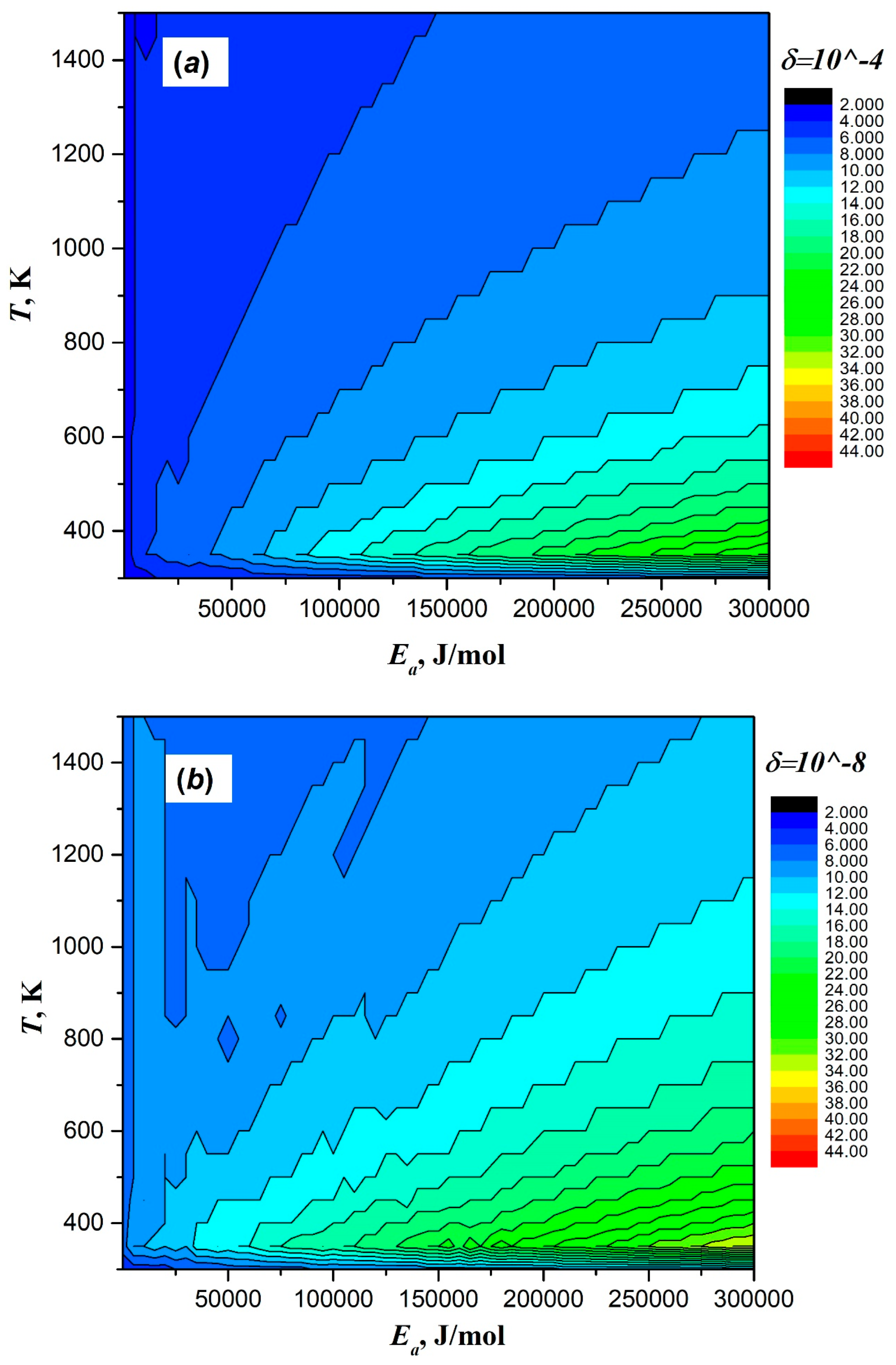

Figure 2.
Three-dimensional image of the integral function of Boltzmann factor.


Table 1.
The integral values of Boltzmann factor with varying Taylor order n.
| Taylor Order n | Ea = 2 J/mol | Ea = 200 J/mol | Ea = 20,000 J/mol | Ea = 200,000 J/mol | ||||
|---|---|---|---|---|---|---|---|---|
| T = 600 K | T = 1200 K | T = 600 K | T = 1200 K | T = 600 K | T = 1200 K | T = 600 K | T = 1200 K | |
| 1 | 301.82115578 | 901.64929838 | 284.65221331 | 867.71805582 | 1.47187736 | 41.45574855 | 1.11339239 × 10⁻¹⁷ | 6.64568260 × 10⁻⁸ |
| 2 | 301.83262904 | 901.66613166 | 285.72844879 | 869.31399874 | 1.84315996 | 44.66857854 | 2.03501118 × 10⁻¹⁷ | 9.66472837 × 10⁻⁸ |
| 3 | 301.83160096 | 901.66487181 | 285.63545060 | 869.19891467 | 1.88712698 | 44.76038220 | 3.15684847 × 10⁻¹⁷ | 1.05477139 × 10⁻⁷ |
| 4 | 301.83170869 | 901.66499125 | 285.64482423 | 869.20938372 | 1.88871043 | 44.75981330 | 4.17892561 × 10⁻¹⁷ | 1.07227989 × 10⁻⁷ |
| 5 | 301.83169624 | 901.66497815 | 285.64378407 | 869.20828368 | 1.88857776 | 44.75969041 | 4.88644170 × 10⁻¹⁷ | 1.07474026 × 10⁻⁷ |
| δ | 4.12482 × 10⁻⁸ | 1.5 × 10⁻⁸ | 3.6 × 10⁻⁶ | 1.3 × 10⁻⁶ | 7 × 10⁻⁵ | 2.7 × 10⁻⁶ | 0.144792 | 0.002289 |
| 6 | 301.83169778 | 901.66497973 | 285.64390756 | 869.20841067 | 1.88857039 | 44.75968614 | 5.27169484 × 10⁻¹⁷ | 1.07498862 × 10⁻⁷ |
| 7 | 301.83169758 | 901.66497953 | 285.64389214 | 869.20839504 | 1.88857151 | 44.75968706 | 5.44047391 × 10⁻¹⁷ | 1.07500633 × 10⁻⁷ |
| 8 | 301.83169761 | 901.66497955 | 285.64389414 | 869.20839705 | 1.88857153 | 44.75968709 | 5.50078992 × 10⁻¹⁷ | 1.07500716 × 10⁻⁷ |
| 9 | 301.83169761 | 901.66497955 | 285.64389388 | 869.20839679 | 1.88857152 | 44.75968708 | 5.51849690 × 10⁻¹⁷ | 1.07500718 × 10⁻⁷ |
| 10 | 301.83169761 | 901.66497955 | 285.64389391 | 869.20839682 | 1.88857152 | 44.75968708 | 5.52277114 × 10⁻¹⁷ | 1.07500718 × 10⁻⁷ |
| δ | 0 | 0 | 1.05 × 10⁻¹⁰ | 3.45 × 10⁻¹¹ | 0 | 0 | 0.000774 | 0 |
| 11 | 301.83169761 | 901.66497955 | 285.64389391 | 869.20839682 | 1.88857152 | 44.75968708 | 5.52361451 × 10⁻¹⁷ | 1.07500718 × 10⁻⁷ |
| 12 | 301.83169761 | 901.66497955 | 285.64389391 | 869.20839682 | 1.88857152 | 44.75968708 | 5.52374846 × 10⁻¹⁷ | 1.07500718 × 10⁻⁷ |
| 13 | 301.83169761 | 901.66497955 | 285.64389391 | 869.20839682 | 1.88857152 | 44.75968708 | 5.52376503 × 10⁻¹⁷ | 1.07500718 × 10⁻⁷ |
| 14 | 301.83169761 | 901.66497955 | 285.64389391 | 869.20839682 | 1.88857152 | 44.75968708 | 5.52376652 × 10⁻¹⁷ | 1.07500718 × 10⁻⁷ |
| 15 | 301.83169761 | 901.66497955 | 285.64389391 | 869.20839682 | 1.88857152 | 44.75968708 | 5.52376660 × 10⁻¹⁷ | 1.07500718 × 10⁻⁷ |
| δ | 0 | 0 | 0 | 0 | 0 | 0 | 1.45 × 10⁻⁸ | 0 |
| 16 | 301.83169761 | 901.66497955 | 285.64389391 | 869.20839682 | 1.88857152 | 44.75968708 | 5.52376660 × 10⁻¹⁷ | 1.07500718 × 10⁻⁷ |
| 17 | 301.83169761 | 901.66497955 | 285.64389391 | 869.20839682 | 1.88857152 | 44.75968708 | 5.52376660 × 10⁻¹⁷ | 1.07500718 × 10⁻⁷ |
| 18 | 301.83169761 | 901.66497955 | 285.64389391 | 869.20839682 | 1.88857152 | 44.75968708 | 5.52376660 × 10⁻¹⁷ | 1.07500718 × 10⁻⁷ |
| 19 | 301.83169761 | 901.66497955 | 285.64389391 | 869.20839682 | 1.88857152 | 44.75968708 | 5.52376660 × 10⁻¹⁷ | 1.07500718 × 10⁻⁷ |
| 20 | 301.83169761 | 901.66497955 | 285.64389391 | 869.20839682 | 1.88857152 | 44.75968708 | 5.52376660 × 10⁻¹⁷ | 1.07500718 × 10⁻⁷ |
| δ | 0 | 0 | 0 | 0 | 0 | 0 | 0 | 0 |
Table 2.
Results of the Newton–Leibniz quadrature method.
| Quadrature Node m | Ea = 2 J/mol | Ea = 200 J/mol | Ea = 20,000 J/mol | Ea = 200,000 J/mol | ||||
|---|---|---|---|---|---|---|---|---|
| T = 600 K | T = 1200 K | T = 600 K | T = 1200 K | T = 600 K | T = 1200 K | T = 600 K | T = 1200 K | |
| 1 × 10² | 304.84987233 | 910.68041913 | 288.48730649 | 877.78754503 | 1.91652897 | 45.37009283 | 6.12793756 × 10⁻¹⁷ | 1.16596876 × 10⁻⁷ |
| 1 × 10³ | 302.13351522 | 902.56652506 | 285.92824787 | 870.06645411 | 1.89135955 | 44.82059549 | 5.58241547 × 10⁻¹⁷ | 1.08390284 × 10⁻⁷ |
| δ | −0.008990585 | −0.00899 | −0.00895 | −0.00887 | −0.01331 | −0.01226 | −0.09772 | −0.07571 |
| 1 × 10⁴ | 301.86187937 | 901.75513412 | 285.67232943 | 869.29420397 | 1.88885024 | 44.76577660 | 5.52961379 × 10⁻¹⁷ | 1.07589474 × 10⁻⁷ |
| δ | −0.000899059 | −0.0009 | −0.0009 | −0.00089 | −0.00133 | −0.00122 | −0.00946 | −0.00739 |
| 1 × 10⁵ | 301.83471578 | 901.67399501 | 285.64673746 | 869.21697755 | 1.88859939 | 44.76029602 | 5.52435114 × 10⁻¹⁷ | 1.07509592 × 10⁻⁷ |
| δ | −8.99949 × 10⁻⁵ | −9 × 10⁻⁵ | −9 × 10⁻⁵ | −8.9 × 10⁻⁵ | −0.00013 | −0.00012 | −0.00095 | −0.00074 |
| 1 × 10⁶ | 301.83199942 | 901.66588110 | 285.64417826 | 869.20925489 | 1.88857430 | 44.75974797 | 5.52382505 × 10⁻¹⁷ | 1.07501606 × 10⁻⁷ |
| δ | −8.99949 × 10⁻⁶ | −9 × 10⁻⁶ | −9 × 10⁻⁶ | −8.9 × 10⁻⁶ | −1.3 × 10⁻⁵ | −1.2 × 10⁻⁵ | −9.5 × 10⁻⁵ | −7.4 × 10⁻⁵ |
Table 3.
Expressions of the approximation for temperature integral.
| Model | Approximation | P(x) |
|---|---|---|
| D | Doyle [32] | |
| CR | Coats and Redfern [12] | |
| G1 | Gorbachev (1st degree) [33] | |
| SY4 | Senum and Yang (4th degree) [21] | |
| PC8 | Perez-Maqueda and Criado (8th degree) [34] | |
| US4 | Urbanovici and Segal IV [35] | |
| CL | Chen and Liu [36] | |
| O3 | Órfão III [17] | |
| J3 | Ji III [37] |
Table 4.
The temperature integral value calculated by the present method and the other approximation methods.
Table 4.
The temperature integral value calculated by the present method and the other approximation methods.
| X = Ea/(RT) (T = 600 K) | MTALAB | Present Solution (n = 10) | Numerical Quadrature | D | CR | G1 | SY4 | PC8 | US4 | CL | O3 | J3 |
|---|---|---|---|---|---|---|---|---|---|---|---|---|
| 1 | 7.8106 × 101 | 7.8106 × 101 | 8.9108 × 101 | 6.6486 × 10⁻¹ | −2.2086 × 10² | 6.3661 × 101 | 7.7575 × 101 | 7.8076 × 101 | 7.6156 × 101 | 9.8401 × 101 | 7.8106 × 101 | 7.8362 × 101 |
| 2 | 2.1597 × 101 | 2.1597 × 101 | 2.2517 × 101 | 6.2429 × 10⁻¹ | −6.6416 × 101 | 1.9419 × 101 | 2.1575 × 101 | 2.1597 × 101 | 2.1429 × 101 | 2.8311 × 101 | 2.1597 × 101 | 2.1601 × 101 |
| 4 | 1.9093 × 100 | 1.9093 × 100 | 1.9187 × 100 | 1.7034 × 10⁻¹ | 1.3648 × 100 | 1.8221 × 100 | 1.9092 × 100 | 1.9093 × 100 | 1.9059 × 100 | 2.5173 × 100 | 1.9093 × 100 | 1.9094 × 100 |
| 6 | 1.9083 × 10⁻¹ | 1.9083 × 10⁻¹ | 1.9096 × 10⁻¹ | 3.1556 × 10⁻² | 1.6513 × 10⁻¹ | 1.8579 × 10⁻¹ | 1.9083 × 10⁻¹ | 1.9083 × 10⁻¹ | 1.9071 × 10⁻¹ | 2.4537 × 10⁻¹ | 1.9083 × 10⁻¹ | 1.9083 × 10⁻¹ |
| 8 | 2.0481 × 10⁻² | 2.0481 × 10⁻² | 2.0490 × 10⁻² | 5.1394 × 10⁻³ | 1.8868 × 10⁻² | 2.0126 × 10⁻² | 2.0481 × 10⁻² | 2.0481 × 10⁻² | 2.0475 × 10⁻² | 2.5632 × 10⁻² | 2.0481 × 10⁻² | 2.0481 × 10⁻² |
| 10 | 2.2981 × 10⁻³ | 2.2981 × 10⁻³ | 2.2982 × 10⁻³ | 7.8368 × 10⁻⁴ | 2.1792 × 10⁻³ | 2.2700 × 10⁻³ | 2.2981 × 10⁻³ | 2.2981 × 10⁻³ | 2.2978 × 10⁻³ | 2.8087 × 10⁻³ | 2.2981 × 10⁻³ | 2.2981 × 10⁻³ |
| 12 | 2.6575 × 10⁻⁴ | 2.6575 × 10⁻⁴ | 2.6576 × 10⁻⁴ | 1.1470 × 10⁻⁴ | 2.5601 × 10⁻⁴ | 2.6332 × 10⁻⁴ | 2.6575 × 10⁻⁴ | 2.6575 × 10⁻⁴ | 2.6572 × 10⁻⁴ | 3.1836 × 10⁻⁴ | 2.6575 × 10⁻⁴ | 2.6575 × 10⁻⁴ |
| 14 | 3.1404 × 10⁻⁵ | 3.1404 × 10⁻⁵ | 3.1402 × 10⁻⁵ | 1.6322 × 10⁻⁵ | 3.0546 × 10⁻⁵ | 3.1182 × 10⁻⁵ | 3.1404 × 10⁻⁵ | 3.1404 × 10⁻⁵ | 3.1402 × 10⁻⁵ | 3.6997 × 10⁻⁵ | 3.1404 × 10⁻⁵ | 3.1404 × 10⁻⁵ |
| 16 | 3.7724 × 10⁻⁶ | 3.7724 × 10⁻⁶ | 3.7724 × 10⁻⁶ | 2.2751 × 10⁻⁶ | 3.6926 × 10⁻⁶ | 3.7512 × 10⁻⁶ | 3.7724 × 10⁻⁶ | 3.7724 × 10⁻⁶ | 3.7723 × 10⁻⁶ | 4.3821 × 10⁻⁶ | 3.7724 × 10⁻⁶ | 3.7724 × 10⁻⁶ |
| 18 | 4.5901 × 10⁻⁷ | 4.5901 × 10⁻⁷ | 4.5900 × 10⁻⁷ | 3.1218 × 10⁻⁷ | 4.5126 × 10⁻⁷ | 4.5690 × 10⁻⁷ | 4.5901 × 10⁻⁷ | 4.5901 × 10⁻⁷ | 4.5900 × 10⁻⁷ | 5.2684 × 10⁻⁷ | 4.5901 × 10⁻⁷ | 4.5901 × 10⁻⁷ |
| 20 | 5.6429 × 10⁻⁸ | 5.6429 × 10⁻⁸ | 5.6430 × 10⁻⁸ | 4.2306 × 10⁻⁸ | 5.5651 × 10⁻⁸ | 5.6213 × 10⁻⁸ | 5.6429 × 10⁻⁸ | 5.6429 × 10⁻⁸ | 5.6428 × 10⁻⁸ | 6.4106 × 10⁻⁸ | 5.6429 × 10⁻⁸ | 5.6429 × 10⁻⁸ |
Table 5.
Standard values of temperature integral calculated by present method.
| T/K | Ea = 2 J/mol | Ea = 20,002 J/mol | Ea = 40,002 J/mol | Ea = 60,002 J/mol | Ea = 80,002 J/mol | Ea = 100,002 J/mol | Ea = 120,002 J/mol | Ea = 140,002 J/mol | Ea = 160,002 J/mol | Ea = 180,002 J/mol | Ea = 200,002 J/mol |
|---|---|---|---|---|---|---|---|---|---|---|---|
| 300 | 1.9984 × 100 | 6.4068 × 10⁻⁴ | 2.0545 × 10⁻⁷ | 6.5897 × 10⁻¹¹ | 2.1142 × 10⁻¹⁴ | 6.7844 × 10⁻¹⁸ | 2.1777 × 10⁻²¹ | 6.9916 × 10⁻²⁵ | 2.2453 × 10⁻²⁸ | 7.2121 × 10⁻³² | 2.3172 × 10⁻³⁵ |
| 318 | 1.9984 × 101 | 8.1688 × 10⁻³ | 3.4100 × 10⁻⁶ | 1.4524 × 10⁻⁹ | 6.3035 × 10⁻¹³ | 2.7834 × 10⁻¹⁶ | 1.2483 × 10⁻¹⁹ | 5.6766 × 10⁻²³ | 2.6130 × 10⁻²⁶ | 1.2157 × 10⁻²⁹ | 5.7090 × 10⁻³³ |
| 336 | 3.7971 × 101 | 1.9709 × 10⁻² | 1.0915 × 10⁻⁵ | 6.3972 × 10⁻⁹ | 3.9296 × 10⁻¹² | 2.5059 × 10⁻¹⁵ | 1.6455 × 10⁻¹⁸ | 1.1055 × 10⁻²¹ | 7.5617 × 10⁻²⁵ | 5.2465 × 10⁻²⁸ | 3.6823 × 10⁻³¹ |
| 354 | 5.5959 × 101 | 3.6632 × 10⁻² | 2.7010 × 10⁻⁵ | 2.1870 × 10⁻⁸ | 1.8958 × 10⁻¹¹ | 1.7247 × 10⁻¹⁴ | 1.6239 × 10⁻¹⁷ | 1.5678 × 10⁻²⁰ | 1.5425 × 10⁻²³ | 1.5400 × 10⁻²⁶ | 1.5556 × 10⁻²⁹ |
| 372 | 7.3947 × 101 | 6.0526 × 10⁻² | 5.9036 × 10⁻⁵ | 6.5170 × 10⁻⁸ | 7.8001 × 10⁻¹¹ | 9.8417 × 10⁻¹⁴ | 1.2870 × 10⁻¹⁶ | 1.7265 × 10⁻¹⁹ | 2.3604 × 10⁻²² | 3.2746 × 10⁻²⁵ | 4.5961 × 10⁻²⁸ |
| 390 | 9.1935 × 101 | 9.3187 × 10⁻² | 1.1877 × 10⁻⁴ | 1.7523 × 10⁻⁷ | 2.8220 × 10⁻¹⁰ | 4.7989 × 10⁻¹³ | 8.4604 × 10⁻¹⁶ | 1.5301 × 10⁻¹⁸ | 2.8199 × 10⁻²¹ | 5.2736 × 10⁻²⁴ | 9.9776 × 10⁻²⁷ |
| 408 | 1.0992 × 1002 | 1.3659 × 10⁻¹ | 2.2414 × 10⁻⁴ | 4.3258 × 10⁻⁷ | 9.1447 × 10⁻¹⁰ | 2.0423 × 10⁻¹² | 4.7284 × 10⁻¹⁵ | 1.1229 × 10⁻¹⁷ | 2.7174 × 10⁻²⁰ | 6.6724 × 10⁻²³ | 1.6574 × 10⁻²⁵ |
| 426 | 1.2791 × 1002 | 1.9288 × 10⁻¹ | 4.0116 × 10⁻⁴ | 9.9213 × 10⁻⁷ | 2.6921 × 10⁻⁹ | 7.7171 × 10⁻¹² | 2.2931 × 10⁻¹⁴ | 6.9882 × 10⁻¹⁷ | 2.1700 × 10⁻¹⁹ | 6.8371 × 10⁻²² | 2.1792 × 10⁻²⁴ |
| 444 | 1.4590 × 1002 | 2.6432 × 10⁻¹ | 6.8611 × 10⁻⁴ | 2.1336 × 10⁻⁶ | 7.2838 × 10⁻⁹ | 2.6265 × 10⁻¹¹ | 9.8160 × 10⁻¹⁴ | 3.7621 × 10⁻¹⁶ | 1.4691 × 10⁻¹⁸ | 5.8205 × 10⁻²¹ | 2.3327 × 10⁻²³ |
| 462 | 1.6389 × 1002 | 3.5330 × 10⁻¹ | 1.1278 × 10⁻³ | 4.3345 × 10⁻⁶ | 1.8290 × 10⁻⁸ | 8.1498 × 10⁻¹¹ | 3.7631 × 10⁻¹³ | 1.7817 × 10⁻¹⁵ | 8.5949 × 10⁻¹⁸ | 4.2063 × 10⁻²⁰ | 2.0823 × 10⁻²² |
| 480 | 1.8189 × 1002 | 4.6228 × 10⁻¹ | 1.7901 × 10⁻³ | 8.3718 × 10⁻⁶ | 4.2978 × 10⁻⁸ | 2.3293 × 10⁻¹⁰ | 1.3079 × 10⁻¹² | 7.5303 × 10⁻¹⁵ | 4.4167 × 10⁻¹⁷ | 2.6281 × 10⁻¹⁹ | 1.5817 × 10⁻²¹ |
| 498 | 1.9988 × 1002 | 5.9379 × 10⁻¹ | 2.7540 × 10⁻³ | 1.5456 × 10⁻⁵ | 9.5179 × 10⁻⁸ | 6.1862 × 10⁻¹⁰ | 4.1652 × 10⁻¹² | 2.8751 × 10⁻¹⁴ | 2.0216 × 10⁻¹⁶ | 1.4420 × 10⁻¹⁸ | 1.0404 × 10⁻²⁰ |
| 516 | 2.1787 × 1002 | 7.5038 × 10⁻¹ | 4.1200 × 10⁻³ | 2.7401 × 10⁻⁵ | 1.9987 × 10⁻⁷ | 1.5384 × 10⁻⁹ | 1.2263 × 10⁻¹¹ | 1.0021 × 10⁻¹³ | 8.3418 × 10⁻¹⁶ | 7.0436 × 10⁻¹⁸ | 6.0155 × 10⁻²⁰ |
| 534 | 2.3586 × 1002 | 9.3461 × 10⁻¹ | 6.0104 × 10⁻³ | 4.6837 × 10⁻⁵ | 4.0012 × 10⁻⁷ | 3.6055 × 10⁻⁹ | 3.3646 × 10⁻¹¹ | 3.2183 × 10⁻¹³ | 3.1354 × 10⁻¹⁵ | 3.0985 × 10⁻¹⁷ | 3.0969 × 10⁻¹⁹ |
| 552 | 2.5385 × 1002 | 1.1490 × 100 | 8.5707 × 10⁻³ | 7.7461 × 10⁻⁵ | 7.6707 × 10⁻⁷ | 8.0102 × 10⁻⁹ | 8.6610 × 10⁻¹¹ | 9.5978 × 10⁻¹³ | 1.0833 × 10⁻¹⁴ | 1.2401 × 10⁻¹⁶ | 1.4358 × 10⁻¹⁸ |
| 570 | 2.7184 × 1002 | 1.3962 × 100 | 1.1972 × 10⁻² | 1.2433 × 10⁻⁴ | 1.4140 × 10⁻⁶ | 1.6953 × 10⁻⁸ | 2.1043 × 10⁻¹⁰ | 2.6767 × 10⁻¹² | 3.4675 × 10⁻¹⁴ | 4.5560 × 10⁻¹⁶ | 6.0542 × 10⁻¹⁸ |
| 588 | 2.8984 × 1002 | 1.6786 × 100 | 1.6410 × 10⁻² | 1.9419 × 10⁻⁴ | 2.5151 × 10⁻⁶ | 3.4332 × 10⁻⁸ | 4.8509 × 10⁻¹⁰ | 7.0233 × 10⁻¹² | 1.0355 × 10⁻¹³ | 1.5485 × 10⁻¹⁵ | 2.3418 × 10⁻¹⁷ |
| 606 | 3.0783 × 1002 | 1.9987 × 100 | 2.2112 × 10⁻² | 2.9587 × 10⁻⁴ | 4.3305 × 10⁻⁶ | 6.6785 × 10⁻⁸ | 1.0659 × 10⁻⁹ | 1.7432 × 10⁻¹¹ | 2.9029 × 10⁻¹³ | 4.9027 × 10⁻¹⁵ | 8.3734 × 10⁻¹⁷ |
| 624 | 3.2582 × 1002 | 2.3588 × 100 | 2.9328 × 10⁻² | 4.4062 × 10⁻⁴ | 7.2372 × 10⁻⁶ | 1.2522 × 10⁻⁷ | 2.2419 × 10⁻⁹ | 4.1121 × 10⁻¹¹ | 7.6803 × 10⁻¹³ | 1.4547 × 10⁻¹⁴ | 2.7864 × 10⁻¹⁶ |
| 642 | 3.4382 × 1002 | 2.7613 × 100 | 3.8340 × 10⁻² | 6.4261 × 10⁻⁴ | 1.1769 × 10⁻⁵ | 2.2698 × 10⁻⁷ | 4.5293 × 10⁻⁹ | 9.2588 × 10⁻¹¹ | 1.9271 × 10⁻¹² | 4.0673 × 10⁻¹⁴ | 8.6810 × 10⁻¹⁶ |
| 660 | 3.6181 × 1002 | 3.2084 × 100 | 4.9459 × 10⁻² | 9.1936 × 10⁻⁴ | 1.8663 × 10⁻⁵ | 3.9888 × 10⁻⁷ | 8.8190 × 10⁻⁹ | 1.9973 × 10⁻¹⁰ | 4.6052 × 10⁻¹² | 1.0768 × 10⁻¹³ | 2.5458 × 10⁻¹⁵ |
| 678 | 3.7980 × 1002 | 3.7022 × 100 | 6.3022 × 10⁻² | 1.2921 × 10⁻³ | 2.8918 × 10⁻⁵ | 6.8119 × 10⁻⁷ | 1.6597 × 10⁻⁸ | 4.1417 × 10⁻¹⁰ | 1.0522 × 10⁻¹¹ | 2.7106 × 10⁻¹³ | 7.0607 × 10⁻¹⁵ |
| 696 | 3.9780 × 1002 | 4.2448 × 100 | 7.9394 × 10⁻² | 1.7866 × 10⁻³ | 4.3858 × 10⁻⁵ | 1.1330 × 10⁻⁶ | 3.0267 × 10⁻⁸ | 8.2811 × 10⁻¹⁰ | 2.3065 × 10⁻¹¹ | 6.5139 × 10⁻¹³ | 1.8601 × 10⁻¹⁴ |
| 714 | 4.1579 × 1002 | 4.8382 × 100 | 9.8971 × 10⁻² | 2.4329 × 10⁻³ | 6.5210 × 10⁻⁵ | 1.8388 × 10⁻⁶ | 5.3615 × 10⁻⁸ | 1.6009 × 10⁻⁹ | 4.8659 × 10⁻¹¹ | 1.4995 × 10⁻¹² | 4.6725 × 10⁻¹⁴ |
| 732 | 4.3378 × 1002 | 5.4841 × 100 | 1.2217 × 10⁻¹ | 3.2666 × 10⁻³ | 9.5191 × 10⁻⁵ | 2.9175 × 10⁻⁶ | 9.2446 × 10⁻⁸ | 2.9995 × 10⁻⁹ | 9.9066 × 10⁻¹¹ | 3.3172 × 10⁻¹² | 1.1231 × 10⁻¹³ |
| 750 | 4.5178 × 1002 | 6.1844 × 100 | 1.4944 × 10⁻¹ | 4.3290 × 10⁻³ | 1.3660 × 10⁻⁴ | 4.5323 × 10⁻⁶ | 1.5545 × 10⁻⁷ | 5.4593 × 10⁻⁹ | 1.9514 × 10⁻¹⁰ | 7.0716 × 10⁻¹² | 2.5910 × 10⁻¹³ |
| 768 | 4.6977 × 1002 | 6.9407 × 100 | 1.8124 × 10⁻¹ | 5.6671 × 10⁻³ | 1.9292 × 10⁻⁴ | 6.9041 × 10⁻⁶ | 2.5538 × 10⁻⁷ | 9.6713 × 10⁻⁹ | 3.7276 × 10⁻¹⁰ | 1.4565 × 10⁻¹¹ | 5.7539 × 10⁻¹³ |
| 786 | 4.8777 × 1002 | 7.7547 × 100 | 2.1808 × 10⁻¹ | 7.3347 × 10⁻³ | 2.6845 × 10⁻⁴ | 1.0326 × 10⁻⁵ | 4.1051 × 10⁻⁷ | 1.6707 × 10⁻⁸ | 6.9194 × 10⁻¹⁰ | 2.9052 × 10⁻¹¹ | 1.2332 × 10⁻¹² |
| 804 | 5.0576 × 1002 | 8.6277 × 100 | 2.6045 × 10⁻¹ | 9.3922 × 10⁻³ | 3.6840 × 10⁻⁴ | 1.5183 × 10⁻⁵ | 6.4661 × 10⁻⁷ | 2.8188 × 10⁻⁸ | 1.2505 × 10⁻⁹ | 5.6239 × 10⁻¹¹ | 2.5568 × 10⁻¹² |
| 822 | 5.2376 × 1002 | 9.5613 × 100 | 3.0890 × 10⁻¹ | 1.1908 × 10⁻² | 4.9903 × 10⁻⁴ | 2.1970 × 10⁻⁵ | 9.9934 × 10⁻⁷ | 4.6526 × 10⁻⁸ | 2.2043 × 10⁻⁹ | 1.0586 × 10⁻¹⁰ | 5.1393 × 10⁻¹² |
| 840 | 5.4175 × 1002 | 1.0557 × 101 | 3.6398 × 10⁻¹ | 1.4956 × 10⁻² | 6.6780 × 10⁻⁴ | 3.1317 × 10⁻⁵ | 1.5172 × 10⁻⁶ | 7.5228 × 10⁻⁸ | 3.7955 × 10⁻⁹ | 1.9410 × 10⁻¹⁰ | 1.0035 × 10⁻¹¹ |
| 858 | 5.5975 × 1002 | 1.1615 × 101 | 4.2624 × 10⁻¹ | 1.8620 × 10⁻² | 8.8349 × 10⁻⁴ | 4.4018 × 10⁻⁵ | 2.2653 × 10⁻⁶ | 1.1931 × 10⁻⁷ | 6.3933 × 10⁻⁹ | 3.4725 × 10⁻¹⁰ | 1.9066 × 10⁻¹¹ |
| 876 | 5.7774 × 1002 | 1.2737 × 101 | 4.9628 × 10⁻¹ | 2.2991 × 10⁻² | 1.1564 × 10⁻³ | 6.1058 × 10⁻⁵ | 3.3297 × 10⁻⁶ | 1.8581 × 10⁻⁷ | 1.0549 × 10⁻⁸ | 6.0707 × 10⁻¹⁰ | 3.5313 × 10⁻¹¹ |
| 894 | 5.9574 × 1002 | 1.3925 × 101 | 5.7468 × 10⁻¹ | 2.8168 × 10⁻² | 1.4983 × 10⁻³ | 8.3647 × 10⁻⁵ | 4.8224 × 10⁻⁶ | 2.8447 × 10⁻⁷ | 1.7073 × 10⁻⁸ | 1.0385 × 10⁻⁹ | 6.3849 × 10⁻¹¹ |
| 912 | 6.1373 × 1002 | 1.5179 × 101 | 6.6205 × 10⁻¹ | 3.4258 × 10⁻² | 1.9229 × 10⁻³ | 1.1326 × 10⁻⁴ | 6.8879 × 10⁻⁶ | 4.2858 × 10⁻⁷ | 2.7130 × 10⁻⁸ | 1.7405 × 10⁻⁹ | 1.1286 × 10⁻¹⁰ |
| 930 | 6.3173 × 1002 | 1.6500 × 101 | 7.5901 × 10⁻¹ | 4.1377 × 10⁻² | 2.4458 × 10⁻³ | 1.5167 × 10⁻⁴ | 9.7100 × 10⁻⁶ | 6.3598 × 10⁻⁷ | 4.2375 × 10⁻⁸ | 2.8613 × 10⁻⁹ | 1.9529 × 10⁻¹⁰ |
| 948 | 6.4972 × 1002 | 1.7888 × 101 | 8.6618 × 10⁻¹ | 4.9650 × 10⁻² | 3.0845 × 10⁻³ | 2.0100 × 10⁻⁴ | 1.3520 × 10⁻⁵ | 9.3033 × 10⁻⁷ | 6.5120 × 10⁻⁸ | 4.6192 × 10⁻⁹ | 3.3118 × 10⁻¹⁰ |
| 966 | 6.6772 × 1002 | 1.9345 × 101 | 9.8419 × 10⁻¹ | 5.9209 × 10⁻² | 3.8590 × 10⁻³ | 2.6375 × 10⁻⁴ | 1.8606 × 10⁻⁵ | 1.3426 × 10⁻⁶ | 9.8548 × 10⁻⁸ | 7.3300 × 10⁻⁹ | 5.5104 × 10⁻¹⁰ |
| 984 | 6.8571 × 1002 | 2.0872 × 101 | 1.1137 × 100 | 7.0196 × 10⁻² | 4.7913 × 10⁻³ | 3.4288 × 10⁻⁴ | 2.5324 × 10⁻⁵ | 1.9130 × 10⁻⁶ | 1.4698 × 10⁻⁷ | 1.1444 × 10⁻⁸ | 9.0052 × 10⁻¹⁰ |
| 1002 | 7.0371 × 1002 | 2.2468 × 101 | 1.2553 × 100 | 8.2759 × 10⁻² | 5.9062 × 10⁻³ | 4.4183 × 10⁻⁴ | 3.4108 × 10⁻⁵ | 2.6929 × 10⁻⁶ | 2.1623 × 10⁻⁷ | 1.7594 × 10⁻⁸ | 1.4468 × 10⁻⁹ |
| 1020 | 7.2170 × 1002 | 2.4134 × 101 | 1.4096 × 100 | 9.7058 × 10⁻² | 7.2309 × 10⁻³ | 5.6459 × 10⁻⁴ | 4.5484 × 10⁻⁵ | 3.7473 × 10⁻⁶ | 3.1398 × 10⁻⁷ | 2.6657 × 10⁻⁸ | 2.2872 × 10⁻⁹ |
| 1038 | 7.3970 × 1002 | 2.5872 × 101 | 1.5774 × 100 | 1.1326 × 10⁻¹ | 8.7955 × 10⁻³ | 7.1572 × 10⁻⁴ | 6.0085 × 10⁻⁵ | 5.1581 × 10⁻⁶ | 4.5032 × 10⁻⁷ | 3.9834 × 10⁻⁸ | 3.5609 × 10⁻⁹ |
| 1056 | 7.5770 × 1002 | 2.7680 × 101 | 1.7592 × 100 | 1.3153 × 10⁻¹ | 1.0633 × 10⁻² | 9.0047 × 10⁻⁴ | 7.8665 × 10⁻⁵ | 7.0268 × 10⁻⁶ | 6.3830 × 10⁻⁷ | 5.8746 × 10⁻⁸ | 5.4638 × 10⁻⁹ |
| 1074 | 7.7569 × 1002 | 2.9561 × 101 | 1.9556 × 100 | 1.5206 × 10⁻¹ | 1.2779 × 10⁻² | 1.1248 × 10⁻³ | 1.0212 × 10⁻⁴ | 9.4789 × 10⁻⁶ | 8.9471 × 10⁻⁷ | 8.5562 × 10⁻⁸ | 8.2686 × 10⁻⁹ |
| 1092 | 7.9369 × 1002 | 3.1513 × 101 | 2.1674 × 100 | 1.7504 × 10⁻¹ | 1.5272 × 10⁻² | 1.3954 × 10⁻³ | 1.3149 × 10⁻⁴ | 1.2667 × 10⁻⁵ | 1.2409 × 10⁻⁶ | 1.2315 × 10⁻⁷ | 1.2350 × 10⁻⁸ |
| 1110 | 8.1168 × 1002 | 3.3537 × 101 | 2.3952 × 100 | 2.0067 × 10⁻¹ | 1.8156 × 10⁻² | 1.7199 × 10⁻³ | 1.6801 × 10⁻⁴ | 1.6778 × 10⁻⁵ | 1.7036 × 10⁻⁶ | 1.7524 × 10⁻⁷ | 1.8216 × 10⁻⁸ |
| 1128 | 8.2968 × 1002 | 3.5634 × 101 | 2.6395 × 100 | 2.2914 × 10⁻¹ | 2.1474 × 10⁻² | 2.1067 × 10⁻³ | 2.1310 × 10⁻⁴ | 2.2035 × 10⁻⁵ | 2.3165 × 10⁻⁶ | 2.4671 × 10⁻⁷ | 2.6550 × 10⁻⁸ |
| 1146 | 8.4768 × 1002 | 3.7803 × 101 | 2.9010 × 100 | 2.6067 × 10⁻¹ | 2.5276 × 10⁻² | 2.5652 × 10⁻³ | 2.6840 × 10⁻⁴ | 2.8704 × 10⁻⁵ | 3.1210 × 10⁻⁶ | 3.4376 × 10⁻⁷ | 3.8259 × 10⁻⁸ |
| 1164 | 8.6567 × 1002 | 4.0045 × 101 | 3.1804 × 100 | 2.9548 × 10⁻¹ | 2.9615 × 10⁻² | 3.1059 × 10⁻³ | 3.3578 × 10⁻⁴ | 3.7104 × 10⁻⁵ | 4.1682 × 10⁻⁶ | 4.7432 × 10⁻⁷ | 5.4538 × 10⁻⁸ |
| 1182 | 8.8367 × 1002 | 4.2360 × 101 | 3.4782 × 100 | 3.3380 × 10⁻¹ | 3.4544 × 10⁻² | 3.7402 × 10⁻³ | 4.1741 × 10⁻⁴ | 4.7609 × 10⁻⁵ | 5.5203 × 10⁻⁶ | 6.4836 × 10⁻⁷ | 7.6941 × 10⁻⁸ |
| 1200 | 9.0166 × 1002 | 4.4748 × 101 | 3.7950 × 100 | 3.7584 × 10⁻¹ | 4.0124 × 10⁻² | 4.4808 × 10⁻³ | 5.1571 × 10⁻⁴ | 6.0659 × 10⁻⁵ | 7.2526 × 10⁻⁶ | 8.7835 × 10⁻⁷ | 1.0748 × 10⁻⁷ |
Disclaimer/Publisher’s Note: The statements, opinions and data contained in all publications are solely those of the individual author(s) and contributor(s) and not of MDPI and/or the editor(s). MDPI and/or the editor(s) disclaim responsibility for any injury to people or property resulting from any ideas, methods, instructions or products referred to in the content. |
© 2023 by the authors. Licensee MDPI, Basel, Switzerland. This article is an open access article distributed under the terms and conditions of the Creative Commons Attribution (CC BY) license (https://creativecommons.org/licenses/by/4.0/).
Share and Cite
MDPI and ACS Style
Zhang, W.; Zheng, Q.; Yu, X.; Shen, Y.; Li, K. Numerical Calculation and 3-D Imaging of the Arrhenius Temperature Integral. Separations 2023, 10, 480. https://doi.org/10.3390/separations10090480
AMA Style
Zhang W, Zheng Q, Yu X, Shen Y, Li K. Numerical Calculation and 3-D Imaging of the Arrhenius Temperature Integral. Separations. 2023; 10(9):480. https://doi.org/10.3390/separations10090480
Chicago/Turabian StyleZhang, Wei, Qiaoyu Zheng, Xiaobing Yu, Yansong Shen, and Kui Li. 2023. "Numerical Calculation and 3-D Imaging of the Arrhenius Temperature Integral" Separations 10, no. 9: 480. https://doi.org/10.3390/separations10090480
Note that from the first issue of 2016, this journal uses article numbers instead of page numbers. See further details here.