Convective Flow in an Aquifer Layer

Abstract

Here, we investigate weakly nonlinear hydrothermal two-dimensional convective flow in a horizontal aquifer layer with horizontal isothermal and rigid boundaries. We treat such a layer as a porous medium, where Darcy’s law holds, subjected to the conditions that the porous layer’s permeability and the thermal conductivity are variable in the vertical direction. This analysis is restricted to the case that the subsequent hydraulic resistivity and diffusivity have a small rate of change with respect to the vertical variable. Applying the weakly nonlinear approach, we derive various order systems and express their solutions. The solutions for convective flow quantities such as vertical velocity and the temperature that arise as the Rayleigh number exceeds its critical value are computed and presented in graphical form.

1. Introduction

A porous medium is a material that consists of a solid matrix with an interconnected void, and it is characterized by its porosity. Mathematical treatment and research on convection in porous media have been presented in many research articles. Darcy’s law for porous media is the momentum equation, which is analogous to the Navier–Stokes equation. Heat transfer through a porous medium is a very common phenomenon. The natural tendency of fluid to expand when heated causes a density inversion to occur, if the heating is strong enough and a circulatory motion follows, termed convection. Convection in the fluid layer is a well-studied phenomenon, and it occurs in many natural settings: in the atmosphere, in the Earth’s mantle and in many industrial applications including solidification and heating. Convective flows in a horizontal dendritic layer during alloy solidification are known to produce chimneys in the final form of the alloy.

The problem of thermal convection in an aquifer layer that occurs in many application areas, notably in environmental sciences and, in particular, in ground water flow [1,2], is fundamentally a problem within the category of convective flow in a porous medium. The effect of the aquifer nonhomogeneity on the onset of thermal convection, as well as on heat transfer through the aquifer has been analyzed [3]. Many cases of convection through aquifers involve horizontal layers, which are non-homogeneous with variable permeability and thermal conductivity.

Riahi [4] studied convection when the boundaries have finite thermal conductivities. Vafai [5] investigated wall effects due to variable porosity. Riahi [6] used a perturbation approach for three-dimensional convection involving nonuniform temperature. He considered the case of a continuous finite bandwidth of modes [7]. An aquifer model was presented by Fowler [8]. Many studies have been presented by various authors [9,10,11,12,13,14,15] to investigate convection in porous media. The effect of variable permeability in porous media was analyzed analytically and numerically by Rees and Pop [16]. Convection in cavities with conducting boundaries was carried out by Rees and Tyvand [17]. The eigenvalue problem for cavities of various shapes was solved by them numerically. Rees and Barletta [18] described a linear stability analysis of a sloping porous layer with isoflux boundaries. Rees et al. [19,20] studied the effect of x-dependent variation in permeability. Bhatta et al. [21,22,23] studied weakly nonlinear convective flows in mushy layers with and without the magnetic effect and permeable mush-liquid interface. Rees and Barletta [24] analyzed the three-dimensional stability of a finite-amplitude convection in a porous layer heated from below.

The present paper studies the problem of nonlinear thermal convection in a horizontal aquifer layer with horizontal rigid and isothermal boundaries, and the aquifer layer is assumed to have variable permeability and thermal conductivity. The analysis is based on the weakly nonlinear theory [4] for the particular case of convection in a porous medium with rigid and isothermal boundaries and is extended here to porous layers with variable permeability and thermal diffusivity. We restrict our analysis to the non-dimensional form of the governing equations in a porous layer subjected to Darcy’s law, and such a non-dimensional form of the governing system introduces three non-dimensional parameters, which are the Rayleigh number, hydraulic resistivity, which is the ratio of the viscosity to permeability, and non-dimensional thermal diffusivity, which is the ratio of diffusivity to a reference diffusivity at the lower boundary [3]. The last two parameters are assumed to vary in the vertical direction, and the magnitude of the vertical rate of change of each of these two parameters is to be kept small.

We have found some interesting results, and in particular, we found that variations in the hydraulic resistivity or thermal diffusivity introduces asymmetry with respect to the mid-plane in the vertical profiles for the convective flow quantities. For the case where the vertical rate of change of either hydraulic resistivity or thermal diffusivity increases in the upward direction, then the flow appears to be stabilizing, while the flow is destabilizing if such a vertical rate of change decreases in the upward direction.

2. Governing Systems and Solutions

The non-dimensional system can be expressed as:

$$\begin{array}{c}\nabla .\overrightarrow{\mathcal{U}}=0\hfill \end{array}$$

(1)

$$\begin{array}{c}\xi \overrightarrow{\mathcal{U}}-R\mathcal{T}\hat{k}+\nabla \mathcal{P}=0\hfill \end{array}$$

(2)

$$\begin{array}{c}\gamma \frac{\partial \mathcal{T}}{\partial t}+\overrightarrow{\mathcal{U}}·\nabla \mathcal{T}=\nabla ·\left(\zeta \nabla \mathcal{T}\right)\hfill \end{array}$$

(3)

Here, $\overrightarrow{\mathcal{U}}$, $\mathcal{T}$, $\mathcal{P}$, R, $\hat{k}$, t, z, $\xi$, $\gamma$ and $\zeta$ respectively represent the velocity, temperature, pressure, Rayleigh number, unit vector in the upward vertical direction, time, vertical coordinate, hydraulic resistivity, coefficient and diffusivity parameter. The coefficient $\gamma$ is given by Rubin [3].

$$\begin{array}{c}\gamma =\frac{\psi \rho C_w+{\rho }_s{C}_s(1-\psi )}{\rho C_w}\hfill \end{array}$$

where $\psi$ is the porosity, $\rho$ is the fluid density, $C_s,C_w$ are the specific heat of the solid and fluid, respectively, and ${\rho }_s$ denotes the density of the solid fraction.

For small $\delta (\delta \ll 1),$ we write:

$$\begin{array}{c}\xi =1+\delta {\xi }_1\left(z+\frac{1}{2}\right)\hfill \end{array}$$

(4)

$$\begin{array}{c}\zeta =1+\delta {\zeta }_1\left(z+\frac{1}{2}\right)\hfill \end{array}$$

(5)

Here, ${\xi }_1$ and ${\zeta }_1$ are constants.

The boundary conditions are:

$$\begin{array}{c}\mathcal{T}=1, W=0\mathrm{at}z=-\frac{1}{2}\end{array}$$

(6)

$$\begin{array}{c}\mathcal{T}=0, W=0\mathrm{at}z=\frac{1}{2}\end{array}$$

(7)

where W is the vertical component of $\overrightarrow{\mathcal{U}}$.

2.1. Basic State Solutions

These are steady state and horizontally-independent solutions, expressing:

$$\begin{array}{ccc}\hfill {\mathcal{T}}_b={\mathcal{T}}_{b0}+\delta {\mathcal{T}}_{b1},& \overrightarrow{\mathcal{U}}=\overrightarrow{0},& R=R_{00}+\delta R_{01}\hfill \end{array}$$

(8)

To zeroth order in $\delta ,$ we have, ${\mathcal{T}}_b={\mathcal{T}}_b\left(z\right), \frac{d^2{\mathcal{T}}_{b0}}{d{z}^2}=0$. Thus, we have ${\mathcal{T}}_{b0}\left(z\right)=c_{0}z+c_1$ and using the boundary conditions, $c_0=-1, c_1=1/2$, which yield:

$$\begin{array}{c}{\mathcal{T}}_{b0}\left(z\right)=\frac{1}{2}-z\hfill \end{array}$$

(9)

Furthermore $\frac{d^2{\mathcal{T}}_{b1}}{d{z}^2}={\zeta }_1$ yielding us:

$$\begin{array}{c}{\mathcal{T}}_{b1}\left(z\right)=\frac{{\zeta }_1}{2}\left(z^2-\frac{1}{4}\right)\hfill \end{array}$$

(10)

Writing:

$$\begin{array}{c}\left(\overrightarrow{\mathcal{U}}, \mathcal{T}, \mathcal{P}\right)=\left(\overrightarrow{0}, {\mathcal{T}}_b, P_b\right)+\left(\overrightarrow{\mathcal{U}}, \theta , P\right)\hfill \end{array}$$

(11)

and using (11) in (1)–(3), boundary Conditions (6) and (7) and defining $\theta =\left(\mathcal{T}-{\mathcal{T}}_b\right)R,$ we obtain the following:

$$\begin{array}{c}\nabla .\overrightarrow{\mathcal{U}}=0\hfill \end{array}$$

(12)

$$\begin{array}{c}\xi \overrightarrow{\mathcal{U}}-\theta \hat{k}+\nabla P=0\hfill \end{array}$$

(13)

$$\begin{array}{c}\gamma \frac{\partial \theta }{\partial t}+\overrightarrow{\mathcal{U}}·\nabla \theta +RW \frac{d{\mathcal{T}}_b}{dz}=\nabla ·\left(\zeta \nabla \theta \right)\hfill \end{array}$$

(14)

with boundary conditions:

$$\begin{array}{cc}\hfill \theta =W=0& \mathrm{at}z=\pm \frac{1}{2}\end{array}$$

(15)

We simplify (12)–(14) using the general representation:

$$\begin{array}{ccc}\hfill \overrightarrow{\mathcal{U}}& =& \overrightarrow{B} \varphi +\overrightarrow{E} \psi \hfill \end{array}$$

(16)

with:

$$\begin{array}{cc}\hfill & \overrightarrow{B}=\nabla \times \nabla \times \hat{k},\hspace{1em}\overrightarrow{E}=\nabla \times \hat{k}\hfill \end{array}$$

(17)

We have $W=-{▵}_2\varphi$ where ${▵}_2=\frac{{\partial }^2}{\partial x^2}+\frac{{\partial }^2}{\partial y^2}$.

Taking the vertical component of the curl of (13), it can be shown that $\nabla \times \hat{k} \psi ·\overrightarrow{\mathcal{U}}$ must vanish, which yields $\overrightarrow{E} \psi =0.$ Taking the vertical component of the double curl of (13) and the use of (16) and (17) give:

$$\begin{array}{c}{▵}_2\left(\xi {\nabla }^2\varphi +\delta {\xi }_1\frac{\partial \varphi }{\partial z}+\theta \right)=0\hfill \end{array}$$

(18)

$$\begin{array}{c}\zeta {\nabla }^2\theta +\delta {\xi }_1\frac{\partial \theta }{\partial z}+R\frac{d{\mathcal{T}}_b}{dz}\left({▵}_2\varphi \right)=\overrightarrow{B}\varphi ·\nabla \theta +\gamma \frac{\partial \theta }{\partial t}\hfill \end{array}$$

(19)

$$\begin{array}{c}\theta =\varphi =0\hspace{1em}\hspace{1em}\mathrm{at}\hspace{1em}z=\pm \frac{1}{2}\hfill \end{array}$$

(20)

Now, writing:

$$\begin{array}{cc}\left(\begin{array}{c}\theta \\ \varphi \end{array}\right)\hfill & =ϵ\left(\begin{array}{c}{\theta }_{10}+\delta {\theta }_{11}+\dots .\\ {\varphi }_{10}+\delta {\varphi }_{11}+\dots .\end{array}\right)+{ϵ}^2\left(\begin{array}{c}{\theta }_{20}+\delta {\theta }_{21}+\dots .\\ {\varphi }_{20}+\delta {\varphi }_{21}+\dots .\end{array}\right)\\ & +{ϵ}^3\left(\begin{array}{c}{\theta }_{30}+{\theta }_{31}+\dots .\\ {\varphi }_{30}+\delta {\varphi }_{31}+\dots .\end{array}\right)+\dots \dots \hfill \end{array}$$

(21)

$$\begin{array}{c}R=\left(R_{00}+\delta R_{01}+\dots .\right)+ϵ\left(R_{10}+\delta R_{11}+\dots .\right)+{ϵ}^2\left(R_{20}+\delta R_{21}+\dots .\right)+\dots \dots \hfill \end{array}$$

(22)

where $ϵ$ is defined as the amplitude of convection, which is small here.

2.2. Linear Problem (Order ${ϵ}^1{\delta }^0$ and ${ϵ}^1{\delta }^1$)

2.2.1. Zeroth Order

To zeroth order in $\delta$ (to order ${ϵ}^1{\delta }^0$, steady case), we have:

$$\begin{array}{c}{▵}_2\left({\nabla }^2{\varphi }_{10}+{\theta }_{10}\right)=0\hfill \end{array}$$

(23)

$$\begin{array}{c}{\nabla }^2{\theta }_{10}-R_{00}\left({▵}_2{\varphi }_{10}\right)=0\hfill \end{array}$$

(24)

$$\begin{array}{c}{\theta }_{10}={\varphi }_{10}=0\hspace{1em}\hspace{1em}\mathrm{at}\hspace{1em}z=\pm \frac{1}{2}\hfill \end{array}$$

(25)

Solutions are given by:

$$\begin{array}{c}{\theta }_{10}=\sqrt{2} \left({\pi }^2+{\alpha }^2\right)H(x,y) cos\pi z ,{\varphi }_{10}=\sqrt{2} H(x,y) cos\pi z\hfill \end{array}$$

(26)

where:

$$\begin{array}{c}H(x,y)=\sum _{n=-N}^N{c}_n{h}_n=\sum _{n=-N}^N{c}_n{e}^{i {\overrightarrow{K}}_n·\overrightarrow{r}}\hfill \end{array}$$

(27)

and:

$$\begin{array}{c}{▵}_2{h}_n=-{\alpha }^2{h}_n, \sum _{n=-N}^N{c}_n{c}_n^{\ast }=1, c_n^{\ast }=c_{-n}, {\overrightarrow{K}}_n·\hat{k}=0, {\overrightarrow{K}}_{-n}=-{\overrightarrow{K}}_n, \left|{\overrightarrow{K}}_n\right|=\alpha \hfill \end{array}$$

(28)

Furthermore, we have:

$$\begin{array}{c}{R}_{00}=\frac{{\left({\pi }^2+{\alpha }^2\right)}^2}{{\alpha }^2},\hspace{1em}{R}_{00c}=4{\pi }^2,\hspace{1em}{\alpha }_c=\pi \hfill \end{array}$$

(29)

2.2.2. Order of $ϵ\delta$

The system in this case is given by:

$$\begin{array}{c}{▵}_2\left[{\nabla }^2{\varphi }_{11}+{\xi }_1\left\{\frac{\partial {\varphi }_{10}}{\partial z}+\left(z+\frac{1}{2}\right){\nabla }^2{\varphi }_{10}\right\}+{\theta }_{11}\right]=0\hfill \end{array}$$

(30)

$$\begin{array}{c}{\nabla }^2{\theta }_{11}+{\zeta }_1\left\{\frac{\partial {\theta }_{10}}{\partial z}+\left(z+\frac{1}{2}\right){\nabla }^2{\theta }_{10}\right\}-R_{00}\left({▵}_2{\varphi }_{11}\right)\\ +R_{00}{\zeta }_{1}z\left({▵}_2{\varphi }_{10}\right)-R_{01}\left({▵}_2{\varphi }_{10}\right)=0\end{array}$$

(31)

with boundary conditions:

$$\begin{array}{c}{\theta }_{11}={\varphi }_{11}=0\hspace{1em}\hspace{1em}\mathrm{at}\hspace{1em}z=\pm \frac{1}{2}\hfill \end{array}$$

(32)

Multiplying (30) by ${\varphi }_{10}$ and (31) by $-\frac{{\theta }_{10}}{R_{00}}$, then we add them and average over the whole layer; and finally, applying (32), we obtain:

$$\begin{array}{c}-{\alpha }^2〈{\xi }_1{\varphi }_{10}\left\{\frac{\partial {\varphi }_{10}}{\partial z}-\left(z+\frac{1}{2}\right)\left({\pi }^2+{\alpha }^2\right){\varphi }_{10}\right\}〉\hfill \\ \hspace{1em}-\frac{1}{4{\pi }^2}〈{\theta }_{10}\left[{\zeta }_1\left\{\frac{\partial {\theta }_{10}}{\partial z}+\left(z+\frac{1}{2}\right){\nabla }^2{\theta }_{10}+R_{00}z\left({▵}_2{\varphi }_{10}\right)\right\}-R_{01}\left({▵}_2{\varphi }_{10}\right)\right]〉=0\hfill \end{array}$$

(33)

Here, we define $<‥>$ as the total horizontal and vertical average of the aquifer layer.

Since:

$$\begin{array}{c}〈{cos}^2\pi z〉=\frac{1}{2},\hspace{1em}〈cos\pi z sin\pi z〉=0,\hspace{1em}{\int }_{-\frac{1}{2}}^{\frac{1}{2}}z {cos}^2\pi z dz=0,\hfill \end{array}$$

we get:

$$\begin{array}{c}-{\alpha }^2\left(-{\pi }^2{\xi }_1\right)-\frac{1}{4{\pi }^2}\left(2{\pi }^2\right)\left[{\pi }^2{R}_{01}-2{\zeta }_1{\pi }^4\right]=0\hfill \end{array}$$

which yields:

$$\begin{array}{c}{R}_{01}=2{\pi }^2\left({\xi }_1+{\zeta }_1\right)\hfill \end{array}$$

(34)

Using (29) and (34), we find the critical Rayleigh number $R_c$ at the onset of motion to be:

$$\begin{array}{c}{R}_c=4{\pi }^2+2{\pi }^2\left({\xi }_1+{\zeta }_1\right)\delta +O\left({\delta }^2\right)\hfill \end{array}$$

(35)

It is seen from $R_c$ that its value is reduced for negative values of ${\xi }_1$ and ${\zeta }_1,$ while the value of $R_c$ increases for positive values of these two parameters.

Now, from (30) and (31), we can obtain:

$$\begin{array}{ll}{▵}_2& \left[{\nabla }^2{\varphi }_{11}+{\theta }_{11}\right]=-\sqrt{2} {\pi }^4{\xi }_1(2z+1)cos\pi z H(x,y)-\sqrt{2} {\pi }^3{\xi }_{1}sin\pi z H(x,y)\\ & =-\sqrt{2} {\pi }^3{\xi }_1\left[\pi (2z+1)cos\pi z+sin\pi z\right]H(x,y)\hfill \end{array}$$

(36)

$$\begin{array}{c}{\nabla }^2{\theta }_{11}-R_{00}\left({▵}_2{\varphi }_{11}\right)=4\sqrt{2}{\pi }^4{\zeta }_{1}z cos\pi z H(x,y)-\sqrt{2} R_{01}{\pi }^{2}cos\pi z H(x,y)\hfill \\ +2\sqrt{2}{\pi }^4{\zeta }_1(2z+1)cos\pi z H(x,y)+2\sqrt{2} {\pi }^3{\zeta }_{1}sin\pi z H(x,y)\hfill \\ =\sqrt{2} {\pi }^2\left[2\pi {\zeta }_{1}sin\pi z+4{\pi }^2{\zeta }_{1}z cos\pi z-R_{01}cos\pi z+2{\pi }^2{\zeta }_1(2z+1)cos\pi z\right]H(x,y)\hfill \end{array}$$

(37)

Let:

$$\begin{array}{c}\left[\begin{array}{c}{\varphi }_{11}\\ {\theta }_{11}\end{array}\right]=\left[\begin{array}{c}{\hat{\varphi }}_{11}\left(z\right)\\ {\hat{\theta }}_{11}\left(z\right)\end{array}\right]H(x,y)\hfill \end{array}$$

(38)

Then, we have:

$$\begin{array}{c}\left(\frac{d^2}{d{z}^2}-{\pi }^2\right){\hat{\varphi }}_{11}+{\hat{\theta }}_{11}=\sqrt{2} \pi {\xi }_1\left[\pi (2z+1)cos\pi z+sin\pi z\right]\hfill \end{array}$$

(39)

$$\begin{array}{c}\left(\frac{d^2}{d{z}^2}-{\pi }^2\right){\hat{\theta }}_{11}+4{\pi }^4{\hat{\varphi }}_{11}=\sqrt{2} {\pi }^2\left[2\pi {\zeta }_{1}sin\pi z\right.\\ \left.+\left\{8{\pi }^2{\zeta }_{1}z-R_{01}+2{\pi }^2{\zeta }_1\right\}cos\pi z\right]\end{array}$$

(40)

with

$${\hat{\theta }}_{11}={\hat{\varphi }}_{11}=0\hspace{1em}\hspace{1em}\mathrm{at}\hspace{1em}z=\pm \frac{1}{2}$$

(41)

To find the particular solution to (39) and (40), we take $\left(\frac{d^2}{d{z}^2}-{\pi }^2\right)$ of (39) and use (40) to eliminate ${\hat{\theta }}_{11}$, which gives us:

$$\begin{array}{c}{\left(\frac{d^2}{d{z}^2}-{\pi }^2\right)}^2{\hat{\varphi }}_{11}-4{\pi }^4{\hat{\varphi }}_{11}=-\sqrt{2} {\pi }^2\left[2{\zeta }_1\pi sin\pi z\right.\hfill \\ \hspace{1em}\left.+\left\{8{\pi }^2{\zeta }_{1}z-R_{01}+2{\pi }^2{\zeta }_1\right\}cos\pi z\right]+\hfill \\ \hspace{1em}-2\sqrt{2} {\pi }^3{\xi }_1\left[\pi cos\pi z+3sin\pi z+\pi z cos\pi z\right]\hfill \end{array}$$

(42)

Assuming:

$${\hat{\varphi }}_{11}=a_1{z}^{2}sin\pi z+a_{2}z sin\pi z+a_{3}z cos\pi z$$

(43)

We have:

$$\begin{array}{c}\frac{d^2{\hat{\varphi }}_{11}}{d{z}^2}=a_1\left(2sin\pi z+4\pi z cos\pi z-{\pi }^2{z}^{2}sin\pi z\right)\hfill \\ +a_2\left(2\pi cos\pi z-{\pi }^{2}z sin\pi z\right)-a_3\left(2\pi sin\pi z+{\pi }^{2}z cos\pi z\right)\hfill \end{array}$$

(44)

and:

$$\begin{array}{c}\frac{d^4{\hat{\varphi }}_{11}}{d{z}^4}={\pi }^2{a}_1\left(-12sin\pi z-8\pi z cos\pi z+{\pi }^2{z}^{2}sin\pi z\right)\hfill \\ +{\pi }^3{a}_2\left(-4cos\pi z+\pi z sin\pi z\right)\hfill \\ +{\pi }^3{a}_3\left(4sin\pi z+\pi z cos\pi z\right)\hfill \end{array}$$

Using the above in (42) and by setting both sides equal and setting similar coefficients to be equal, we obtain the following:

Coefficients of $z^{2}sin\pi z$ yield:

$${\pi }^4{a}_1-2{\pi }^2\left(-{\pi }^2{a}_1\right)+{\pi }^4{a}_1-4{\pi }^4{a}_1=4{\pi }^4{a}_1-4{\pi }^4{a}_1=0$$

From the coefficients of $zsin\pi z$, we obtain:

$${\pi }^4{a}_2-2{\pi }^2\left(-{\pi }^2{a}_2\right)+{\pi }^4{a}_2-4{\pi }^4{a}_2=0$$

The coefficients of $zcos\pi z$ yield:

$$\begin{array}{c}{a}_1\left(-8{\pi }^3\right)+a_3{\pi }^4-2{\pi }^2\left(4\pi a_1-{\pi }^2{a}_3\right)+{\pi }^4{a}_3-4{\pi }^4{a}_3=-2\sqrt{2}{\pi }^4\left(4{\zeta }_1+{\xi }_1\right)\hfill \\ ⟹a_1=\frac{\pi }{4\sqrt{2}}\left(4{\zeta }_1+{\xi }_1\right)\hfill \end{array}$$

(45)

The coefficients of $sin\pi z$ yield:

$$\begin{array}{c}{a}_1\left(-12{\pi }^2\right)+4a_3{\pi }^3-2{\pi }^2\left(2a_1-2a_3\pi \right)=-2\sqrt{2}{\pi }^3\left({\zeta }_1+3{\xi }_1\right)\hfill \\ ⟹-2a_1+\pi a_3=-\frac{\pi }{2\sqrt{2}}\left({\zeta }_1+3{\xi }_1\right)\hfill \end{array}$$

(46)

The coefficients of $cos\pi z$ yield:

$$\begin{array}{c}{a}_2\left(-4{\pi }^3\right)-2{\pi }^2\left(2a_2\pi \right)=\sqrt{2}{\pi }^2\left(R_{01}-2{\pi }^2{\zeta }_1-2{\pi }^2{\xi }_1\right)\hfill \\ ⟹a_2=\frac{1}{4\sqrt{2}\pi }\left\{2{\pi }^2\left({\zeta }_1+{\xi }_1\right)-R_{01}\right\}=0\hfill \end{array}$$

(47)

Furthermore, we have:

$$\begin{array}{c}{a}_3=\frac{1}{\pi }\left[2a_1-\frac{\pi }{2\sqrt{2}}\left({\zeta }_1+3{\xi }_1\right)\right]=\frac{1}{2\sqrt{2}}\left(3{\zeta }_1-2{\xi }_1\right)\hfill \end{array}$$

(48)

We use (43) and (45)–(47) in (39) to find the particular solution for ${\hat{\theta }}_{11}$.

$$\begin{array}{c}{\hat{\theta }}_{11}=-\left(\frac{d^2}{d{z}^2}-{\pi }^2\right){\hat{\varphi }}_{11}+\sqrt{2} \pi {\xi }_1\left[\pi (2z+1)cos\pi z+sin\pi z\right]\hfill \\ =a_1\left(-2sin\pi z-4\pi z cos\pi z+{\pi }^2{z}^{2}sin\pi z\right)\hfill \\ +a_3\left(2\pi sin\pi z+{\pi }^{2}z cos\pi z\right)+a_1{\pi }^2{z}^{2}sin\pi z\hfill \\ +a_3{\pi }^{2}z cos\pi z+\sqrt{2}\pi {\xi }_1\left[(2z+1)cos\pi z+sin\pi z\right]\hfill \\ =b_1{z}^{2}sin\pi z+b_{2}z sin\pi z+b_{3}z cos\pi z+b_{4}sin\pi z+b_{5}cos\pi z\hfill \end{array}$$

(49)

where:

$$\begin{array}{c}{b}_1=2{\pi }^2{a}_1,b_2=0,b_3=-4\pi a_1+2{\pi }^2{a}_3+2\sqrt{2}{\pi }^2{\xi }_1\hfill \\ b_4=-2a_1+2\pi a_3+\sqrt{2}\pi {\xi }_1,b_5=\sqrt{2}{\pi }^2{\xi }_1\hfill \end{array}$$

(50)

Now, we obtain a complementary solution. Designating $\frac{d{\hat{\varphi }}_{11}}{dz}=S_1, \frac{d{\hat{\theta }}_{11}}{dz}=S_2$, we can write:

$$\begin{array}{c}\frac{d{\hat{\varphi }}_{11}}{dz}=S_1,\frac{d{\hat{\theta }}_{11}}{dz}=S_2,\frac{d{S}_1}{dz}={\pi }^2{\hat{\varphi }}_{11}-{\hat{\theta }}_{11},\frac{d{S}_2}{dz}={\pi }^2{\hat{\theta }}_{11}-4{\pi }^4{\hat{\varphi }}_{11}\hfill \end{array}$$

(51)

and using matrix algebra, (51) can be written in matrix form as:

$$\begin{array}{ccc}\hfill X^{\prime }=AX& \mathrm{where}& A=\left[\begin{array}{cccc}0& 0& 1& 0\\ 0& 0& 0& 1\\ {\pi }^2& -1& 0& 0\\ -4{\pi }^4& {\pi }^2& 0& 0\end{array}\right],X=\left[\begin{array}{c}{\hat{\varphi }}_{11}\\ {\hat{\theta }}_{11}\\ S_1\\ S_2\end{array}\right]\hfill \end{array}$$

(52)

The solution to this homogeneous system is given by:

$$\begin{array}{c}X=K{e}^{\lambda z}\hfill \end{array}$$

(53)

Here, $\lambda$ and K can be obtained from:

$$\begin{array}{c}\det \left(A-\lambda I\right)=0\mathrm{and}\left(A-\lambda I\right)K=0\hfill \end{array}$$

respectively. Now, $\det \left(A-\lambda I\right)=0$ yields:

$$\begin{array}{c}{\lambda }^4-2{\pi }^2{\lambda }^2-3{\pi }^4=0\hfill \\ \Rightarrow {\lambda }^2=-{\pi }^2, 3{\pi }^2\hfill \end{array}$$

Thus, we have four eigenvalues as:

$$\begin{array}{c}{\lambda }_1=i\pi , {\lambda }_2=-i\pi , {\lambda }_3=\sqrt{3}\pi , {\lambda }_4=-\sqrt{3}\pi \hfill \end{array}$$

(54)

Let $K_i={\left[\begin{array}{cccc}{k}_{1i};& k_{2i};& k_{3i};& k_{4i}\end{array}\right]}^T$ be the eigenvector corresponding to eigenvalue ${\lambda }_i, i=1,\dots ,4.$ We have:

$$\left(A-{\lambda }_{i}I\right)K_i=0\hspace{1em}⟹\left\{\begin{array}{c}-{\lambda }_i{k}_{1i}+k_{3i}=0\\ -{\lambda }_i{k}_{2i}+k_{4i}=0\\ {\pi }^2{k}_{1i}-k_{2i}-{\lambda }_i{k}_{3i}=0\\ -4{\pi }^4{k}_{1i}+{\pi }^2{k}_{2i}-{\lambda }_i{k}_{4i}=0\end{array}\right.$$

(55)

Solving this system, we obtain:

$$\begin{array}{c}{k}_{1i}=1,k_{2i}=\frac{4{\pi }^4}{{\pi }^2-{\lambda }_i^2},k_{3i}={\lambda }_i,k_{4i}=\frac{4{\pi }^4{\lambda }_i}{{\pi }^2-{\lambda }_i^2}\hfill \end{array}$$

(56)

and we find four solutions:

$$\begin{array}{c}\left[\begin{array}{c}{\hat{\varphi }}_{11}\\ {\hat{\theta }}_{11}\end{array}\right]={\displaystyle \sum _{i=1}^4}{C}_i{K}_{1i}{e}^{{\lambda }_{i}z}+\left[\begin{array}{c}{a}_1\\ b_1\end{array}\right]z^{2}sin\pi z+\left[\begin{array}{c}{a}_2\\ b_2\end{array}\right]zsin\pi z\\ +\left[\begin{array}{c}{a}_3\\ b_3\end{array}\right]zcos\pi z+\left[\begin{array}{c}0\\ b_4\end{array}\right]sin\pi z+\left[\begin{array}{c}0\\ b_5\end{array}\right]cos\pi z\end{array}$$

where the arbitrary constants $C_{i}i=1,\dots ,4$ can be determined by using the four boundary conditions ${\hat{\theta }}_{11}={\hat{\varphi }}_{11}=0atz=\pm \frac{1}{2}$.

3. Nonlinear Problem

3.1. Order of ${ϵ}^2{\delta }^0$

In this case, we have:

$$\begin{array}{c}{▵}_2\left({\nabla }^2{\varphi }_{20}+{\theta }_{20}\right)=0\hfill \end{array}$$

(57)

$$\begin{array}{c}{\nabla }^2{\theta }_{20}-R_{00}\left({▵}_2{\varphi }_{20}\right)-R_{10}\left({▵}_2{\varphi }_{10}\right)=\overrightarrow{B}{\varphi }_{10}·\nabla {\theta }_{10}\hfill \end{array}$$

(58)

$$\begin{array}{c}{\theta }_{20}={\varphi }_{20}=0\mathrm{at}z=\pm \frac{1}{2}\hfill \end{array}$$

(59)

We consider special solutions ${\varphi }_{10n}, {\theta }_{10n}$ of the linear system at order ${ϵ}^1{\delta }^0$:

$$\begin{array}{c}\left[\begin{array}{c}{\varphi }_{10n}\\ {\theta }_{10n}\end{array}\right]=\left[\begin{array}{c}{\hat{\varphi }}_{10}\left(z\right)\\ {\hat{\theta }}_{10}\left(z\right)\end{array}\right]h_n(x,y)\hfill \end{array}$$

(60)

where:

$$\begin{array}{c}{\hat{\varphi }}_{10}\left(z\right)=\sqrt{2}cos\pi z,{\hat{\theta }}_{10}\left(z\right)=2\sqrt{2}{\pi }^{2}cos\pi z\hfill \end{array}$$

(61)

Multiplying (57) by ${\varphi }_{10n}$ and (58) by $-R_{00}^{-1}{\theta }_{10n}$, adding them and averaging over the whole layer and, finally, applying (32), we obtain:

$$R_{10}=-\frac{〈{\theta }_{10n}\left(\overrightarrow{B}{\varphi }_{10}·\nabla {\theta }_{10}\right)〉}{〈{\theta }_{10n}\left({▵}_2{\varphi }_{10}\right)〉}=0$$

(62)

Multiplying (62) by $C_n$ and taking the summation ${\sum }_{n=-N}^N$, we find:

$$R_{10}=-\frac{1}{2}\frac{〈{\theta }_{10}^2\nabla ·{\overrightarrow{u}}_{10}〉}{〈{\theta }_{10n}\left({▵}_2{\varphi }_{10}\right)〉}$$

(63)

Equations (57)–(59) give the solutions for ${\varphi }_{20}$ and ${\theta }_{20}$:

$$\begin{array}{c}{\varphi }_{20}=\sum _{l,p=-N}^{N}F\left(z,{\hat{\varphi }}_{lp}\right)C_l{C}_p{h}_l{h}_p+G\left(z\right),\hfill \end{array}$$

(64)

$$\begin{array}{c}{\theta }_{20}=-D^{2}G\left(z\right)-\sum _{l,p=-N}^N\left[D^2-2{\pi }^2\left(1+{\hat{\varphi }}_{lp}\right)\right]F\left(z{\hat{\varphi }}_{lp}\right)C_l{C}_p{h}_l{h}_p\hfill \end{array}$$

(65)

where:

$${\hat{\varphi }}_{lp}=\frac{{\overrightarrow{K}}_l·{\overrightarrow{K}}_l}{{\pi }^2},D\equiv \frac{d}{dz}$$

(66)

$$G\left(z\right)=\frac{\pi }{4}sin\pi z,F\left(z,{\hat{\varphi }}_{lp}\right)=\frac{\pi }{4}\frac{\left(1+{\hat{\varphi }}_{lp}\right)sin2\pi z}{\left[2+\left(1+{\hat{\varphi }}_{lp}\right)+\frac{1}{2}{\left(1+{\hat{\varphi }}_{lp}\right)}^2\right]}$$

(67)

For the two-dimensional case, (64)–(67) become (since $N=1,$ $C_l=C_p=1/\sqrt{2},$ $h_1=e^{i\pi x},$ $h_{-1}=e^{-i\pi x},$ $l=\pm 1, p=\pm 1$):

$$\begin{array}{c}{\varphi }_{20}=\frac{\pi }{4}\left(1+\frac{cos2\alpha x}{3}\right)sin2\pi z\end{array}$$

(68)

$$\begin{array}{c}{\theta }_{20}={\pi }^{3}sin2\pi z-\frac{\pi }{6}\left[\frac{d^2}{d{z}^2}-4{\pi }^2\right]\frac{sin2\pi z}{2}cos2\alpha x\\ ={\pi }^3\left(1+\frac{2cos2\alpha x}{3}\right)sin2\pi z\end{array}$$

(69)

3.2. Order of ${ϵ}^2{\delta }^1$

In this case, we have:

$$\begin{array}{c}{▵}_2\left({\nabla }^2{\varphi }_{21}+{\theta }_{21}\right)=0\hfill \end{array}$$

(70)

$$\begin{array}{c}{\nabla }^2{\theta }_{21}-R_{00}\left({▵}_2{\varphi }_{21}\right)=R_{11}\left({▵}_2{\varphi }_{10}\right)+\overrightarrow{B}{\varphi }_{11}·\nabla {\theta }_{10}+\overrightarrow{B}{\varphi }_{10}·\nabla {\theta }_{11}\hfill \end{array}$$

(71)

$$\begin{array}{c}{\theta }_{21}={\varphi }_{21}=0\mathrm{at}z=\pm \frac{1}{2}\hfill \end{array}$$

(72)

Multiplying (70) by ${\varphi }_{10n}$ and (71) by $-R_{00}^{-1}{\theta }_{10n}$, adding them and averaging over the whole layer, we obtain:

$$R_{11}=-\frac{〈{\theta }_{10n}\left(\overrightarrow{B}{\varphi }_{11}·\nabla {\theta }_{10}+\overrightarrow{B}{\varphi }_{10}·\nabla {\theta }_{11}\right)〉}{〈{\theta }_{10n}\left({▵}_2{\varphi }_{10}\right)〉}$$

(73)

where:

$$\begin{array}{c}\overrightarrow{B}\varphi ·\nabla \theta \equiv \frac{{\partial }^2\varphi }{\partial x\partial z}\frac{\partial \theta }{\partial x}+\frac{{\partial }^2\varphi }{\partial y\partial z}\frac{\partial \theta }{\partial y}-\left({▵}_2\varphi \right)\frac{\partial \theta }{\partial z}\hfill \\ \equiv u\frac{\partial \theta }{\partial x}+v\frac{\partial \theta }{\partial y}+w\frac{\partial \theta }{\partial z}\hfill \end{array}$$

(74)

For two-dimensional flow, $R_{11}=0.$ The present work presents the two-dimensional case, but we have provided the formulation for a general three-dimensional study so that it can be useful for future extension.

Next, the solvability condition at order ${ϵ}^3$ yields:

$$-R_{20}〈{\theta }_{10n}^{\ast }\left({▵}_2{\varphi }_{10}\right)〉=\left[〈{\theta }_{10n}^{\ast }\left(\overrightarrow{B}{\varphi }_{10}·\nabla {\theta }_{20}+\overrightarrow{B}{\varphi }_{20}·\nabla {\theta }_{10}\right)〉\right]$$

(75)

Furthermore, the heat flux (heat transported by convection) can be estimated as follows:

$$\mathrm{Heat} \mathrm{Flux}=H_c=〈w\theta 〉\approx {\alpha }^2\left(R-R_{00}-\delta R_{01}\right)\frac{〈{\hat{\varphi }}_{10}{\hat{\theta }}_{10}〉}{R_{20}}$$

(76)

For the two-dimensional case:

$$H_c=2\left(R-4{\pi }^2-\delta R_{01}\right),R_{20}={\pi }^4$$

(77)

Using (34) in (77), we find that for the given value of R, the heat flux is higher for negative values of ${\xi }_1$ and ${\zeta }_1,$ while the heat flux is lower for positive values of these parameters.

4. Results

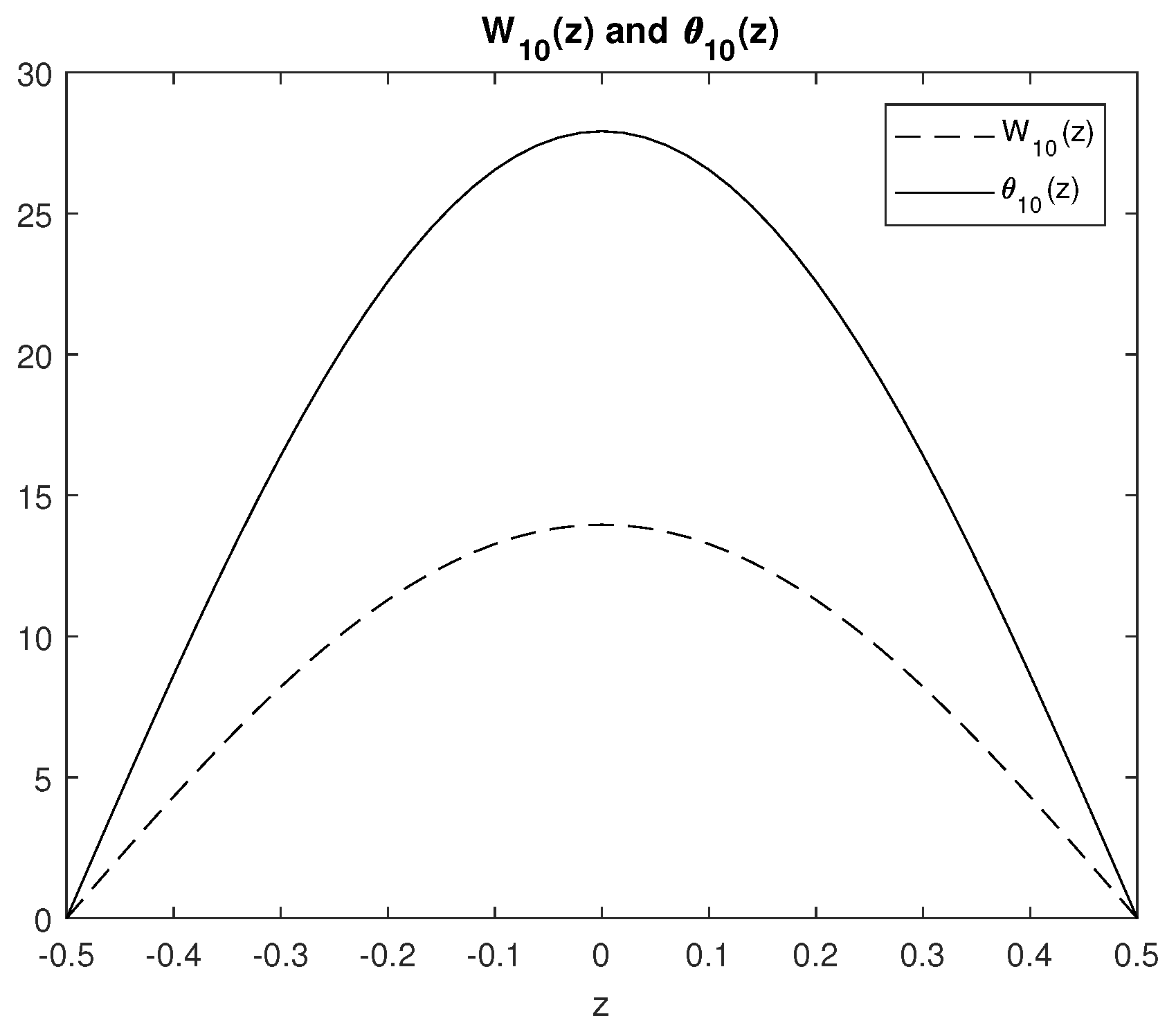
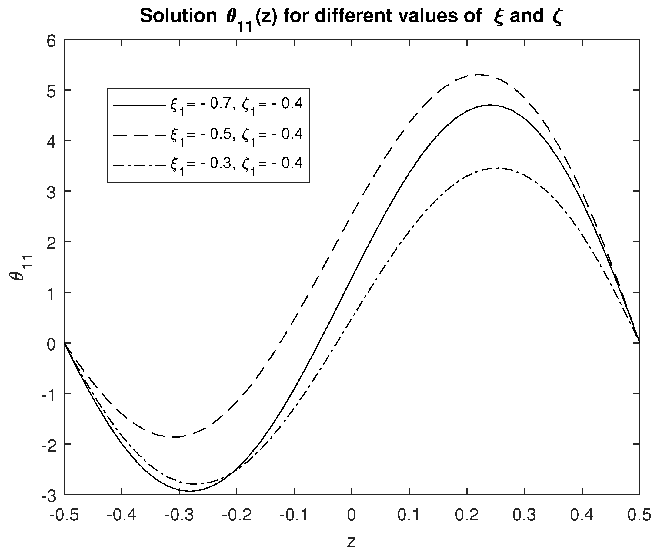
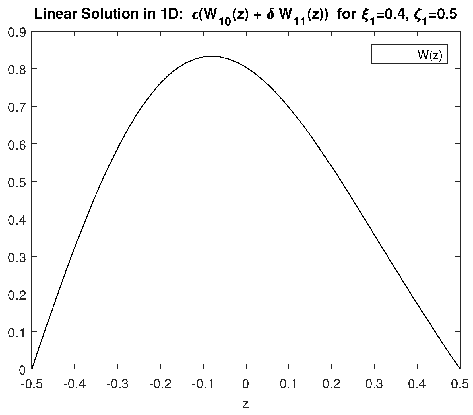
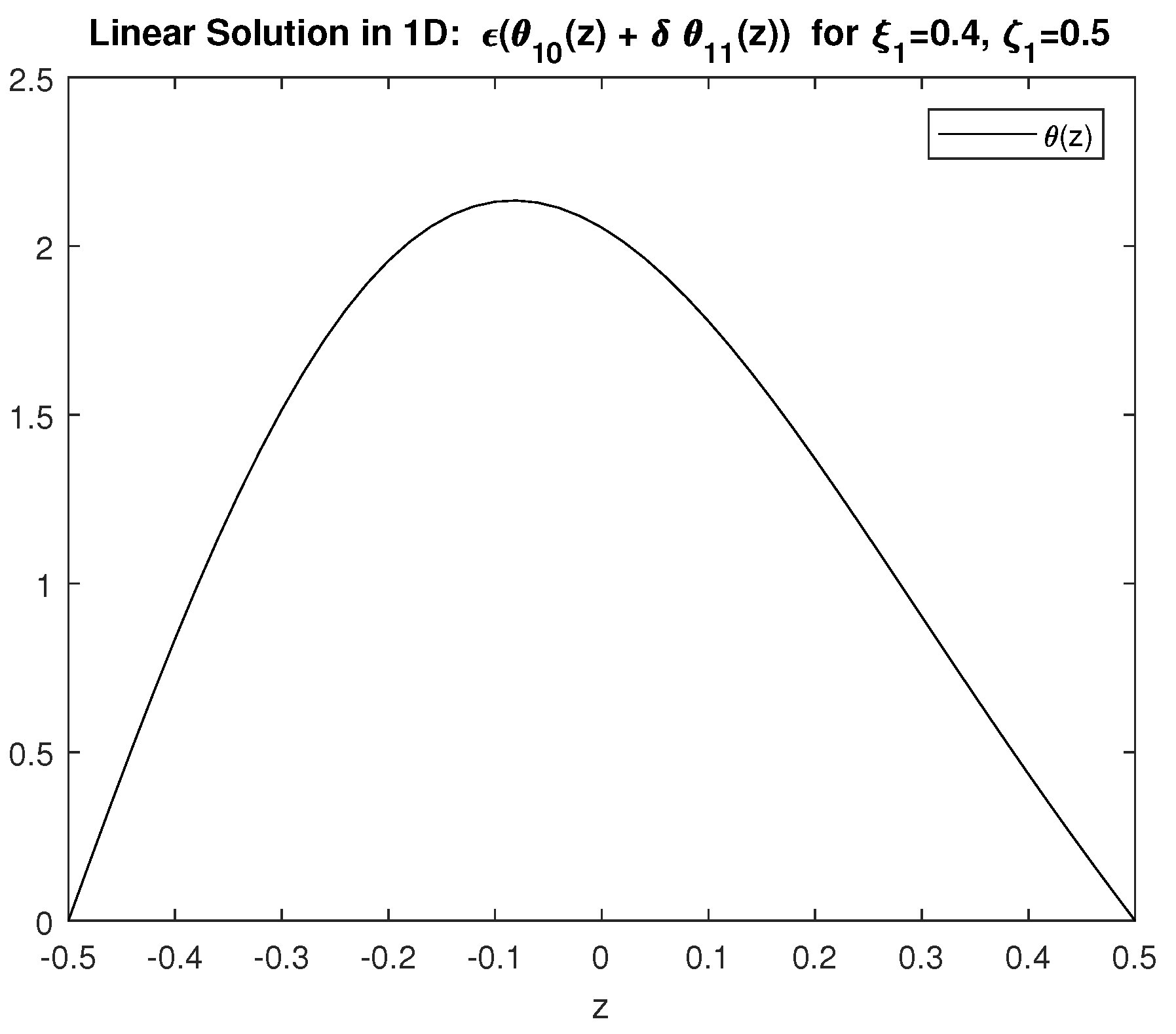
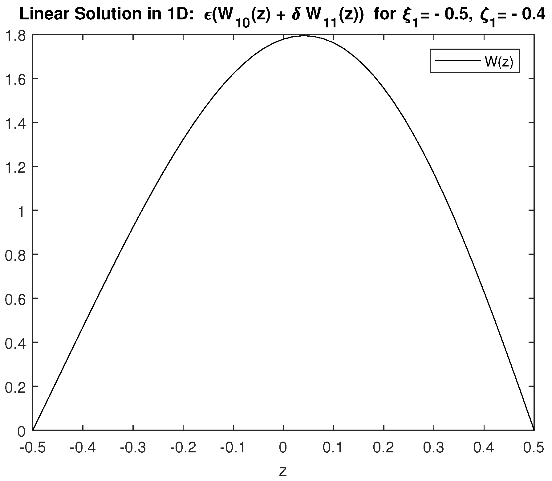
4.1. One-Dimensional Results for the Vertical Dependence of Linear Solutions:

In all our computations, the values of $\delta$ and $ϵ$ used are 0.8 and 0.1, respectively. We have chosen 0.8 as the value of $\delta ,$ even though it is assumed mathematically that $\delta \ll 1,$ in order to make the effects due to variable hydraulic resistivity and diffusivity more visible in the graphs of the figures. Similar types of graphical considerations are made in other research areas. For example, Anderson and Worster [25] studied thin mushy layers with thickness $\delta \ll 1,$ but in their graphical representations, they chose $\delta =0.5$ in order to show more visibly the effect of $\delta$ in their results.

The zeroth order solutions $W_{10}\left(z\right)$ and ${\theta }_{10}\left(z\right)$ are displayed below in Figure 1.

It can be seen from this figure that vertical profiles of the linear flow quantities to zeroth order in $\delta$, which are independent of ${\xi }_1$ and ${\zeta }_1,$ are symmetric with respect to mid-plane at $z=0.$ The following graph in Figure 2 displays $W_{11}\left(z\right)$, whereas Figure 3 displays ${\theta }_{11}\left(z\right)$ for different ${\xi }_1$ keeping ${\zeta }_1$ fixed for positive values of ${\xi }_1$ and ${\zeta }_1$.

It can be seen from Figure 2 and Figure 3 that vertical profiles for flow quantities to first order in $\delta$, which are dependent on ${\xi }_1$ and ${\zeta }_1,$ have lost their symmetry with respect to mid-plane flow and are stabilizing for ${\xi }_1>0.$ The following graph in Figure 4 displays $W_{11}\left(z\right)$, whereas Figure 5 displays ${\theta }_{11}\left(z\right)$ for different values of ${\xi }_1$ keeping ${\zeta }_1$ fixed for negative values of ${\xi }_1$ and ${\zeta }_1$.

A similar asymmetry property holds here for Figure 4 and Figure 5. Figure 6 and Figure 7 present the linear solutions $ϵ\left(W_{10}\left(z\right)+\delta W_{11}\left(z\right)\right)$ and $ϵ\left({\theta }_{10}\left(z\right)+\delta {\theta }_{11}\left(z\right)\right)$ with ${\xi }_1=0.4$ and ${\zeta }_1=0.5$.

It can be seen from Figure 6 and Figure 7 that the vertical profiles of linear flow quantities up to order ${\delta }^2$ are slightly asymmetric due to the order $\delta$ quantities. Similar asymmetry is evident in Figure 8 and Figure 9. Figure 8 and Figure 9 present the linear solutions $ϵ\left(W_{10}\left(z\right)+\delta W_{11}\left(z\right)\right)$ and $ϵ\left({\theta }_{10}\left(z\right)+\delta {\theta }_{11}\left(z\right)\right)$ with ${\xi }_1=-0.5$ and ${\zeta }_1=-0.4$.

It can be seen from the presented linear results for the vertical dependence of the vertical velocity that for positive values of the vertical rate of change of the aquifer parameters (hydraulic resistivity and diffusivity), the magnitude of the vertical velocity decreases, which can imply flow stability, while an instability of the flow can result if such a vertical rate of change of the aquifer parameters is negative.

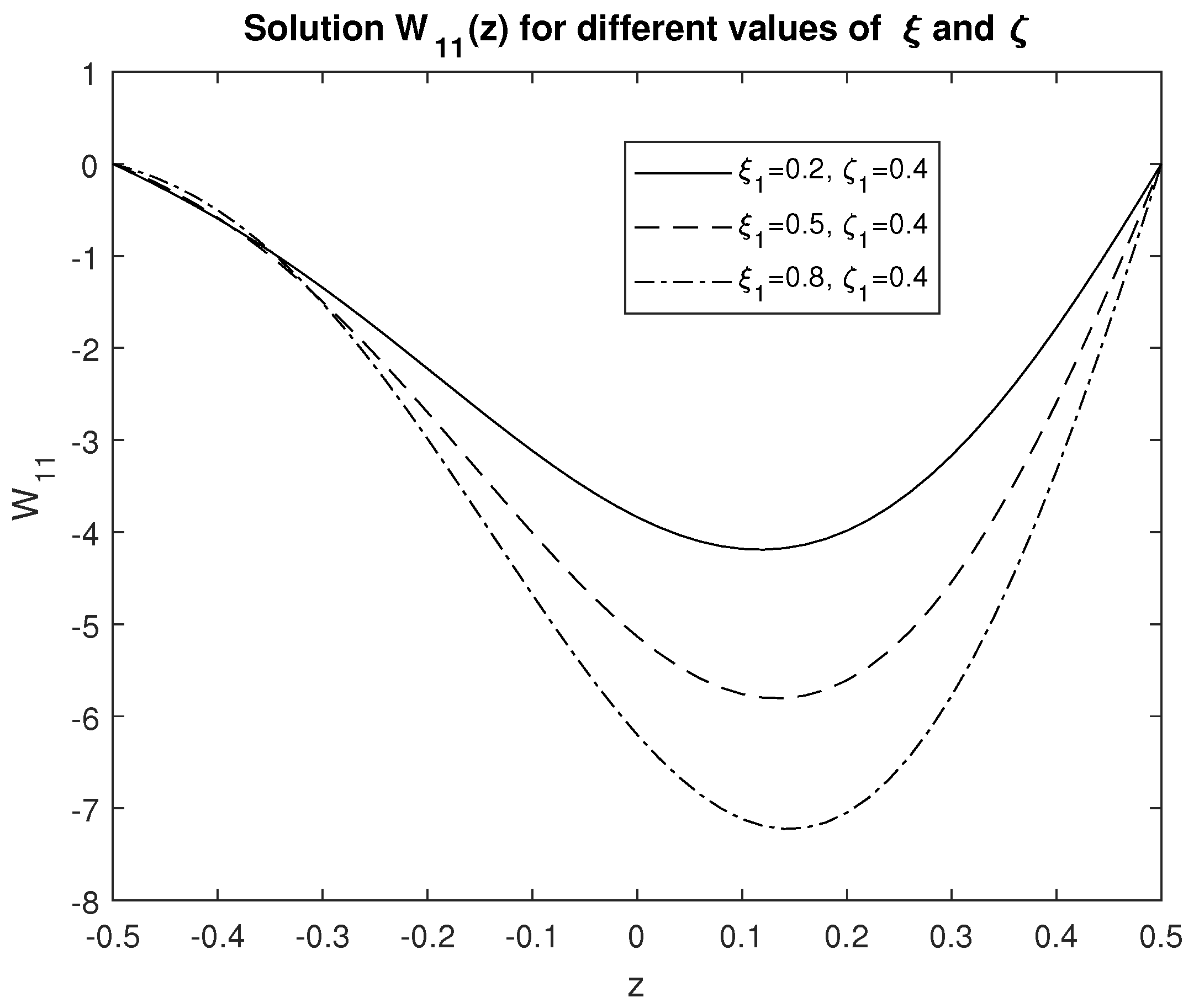
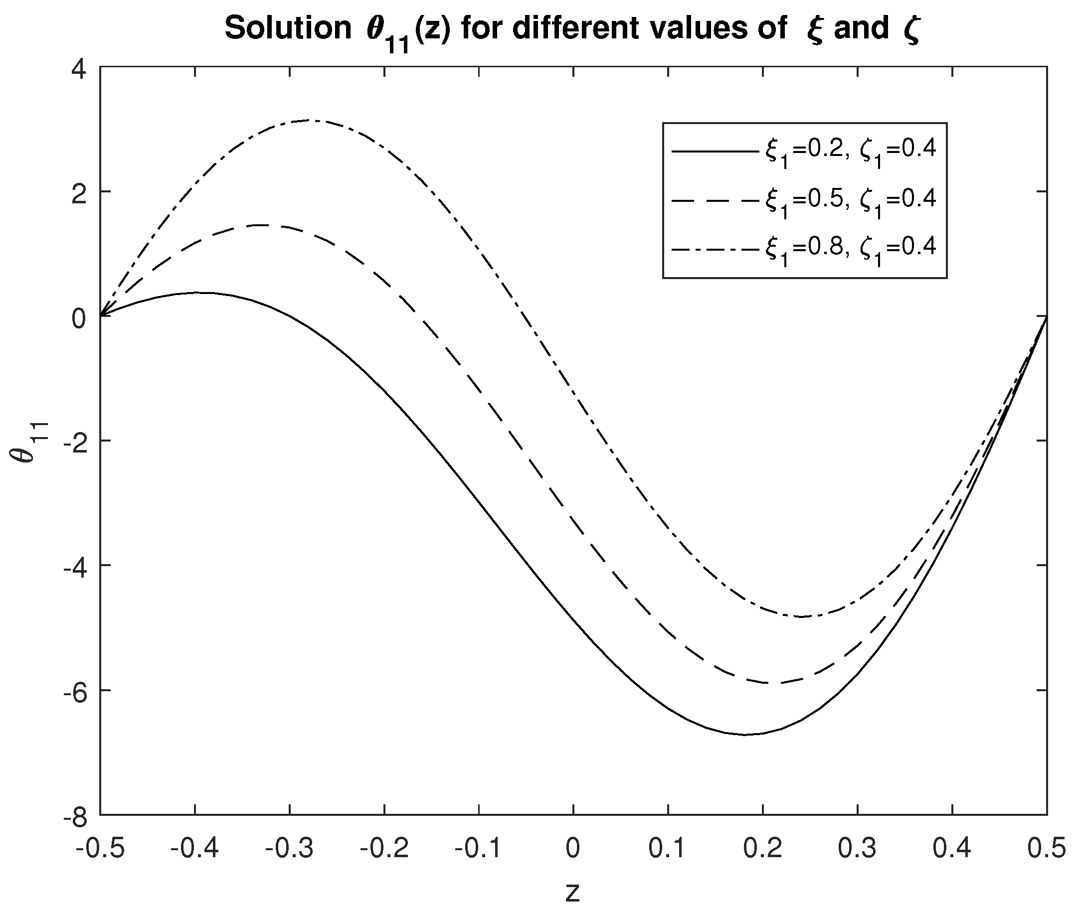
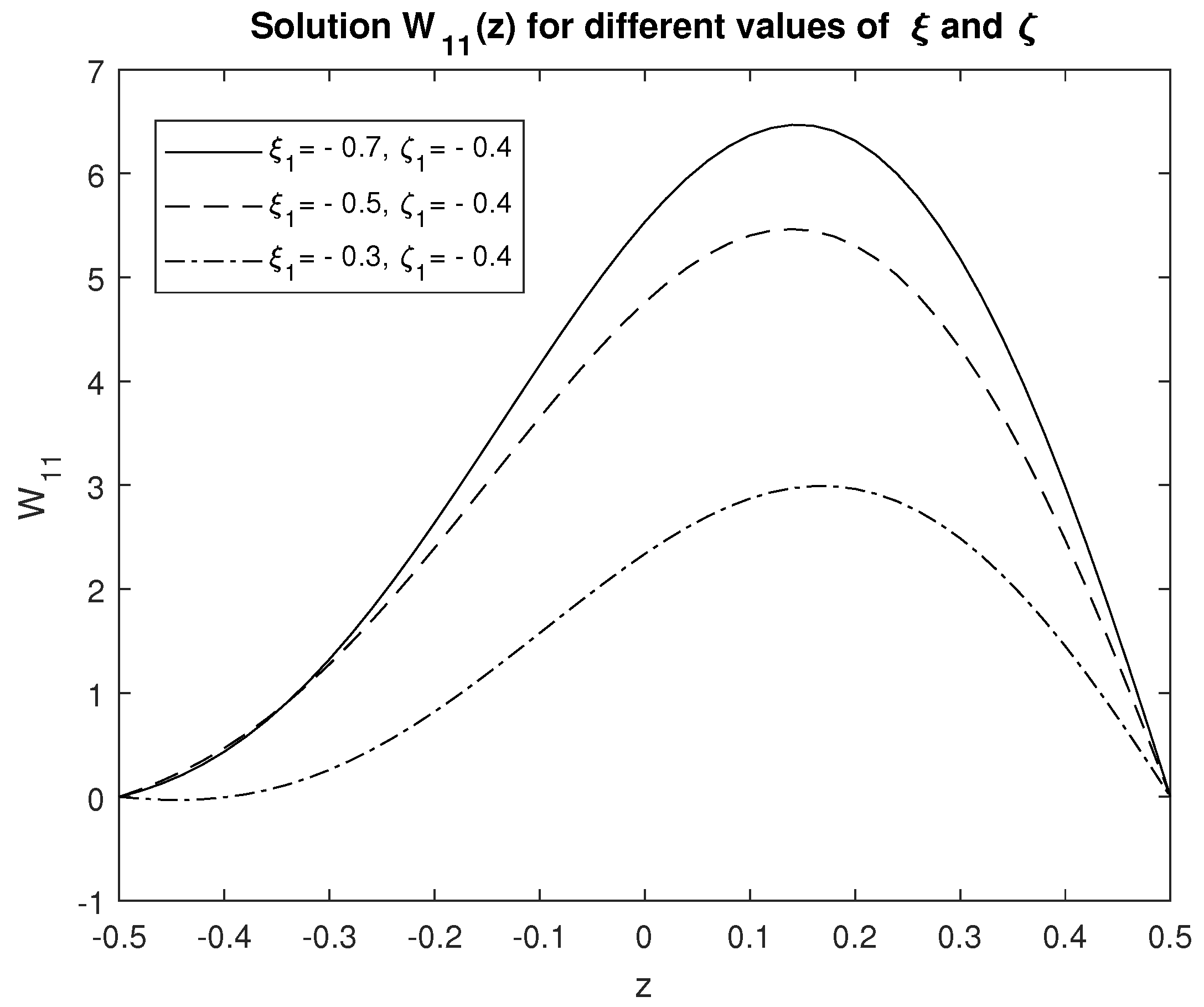
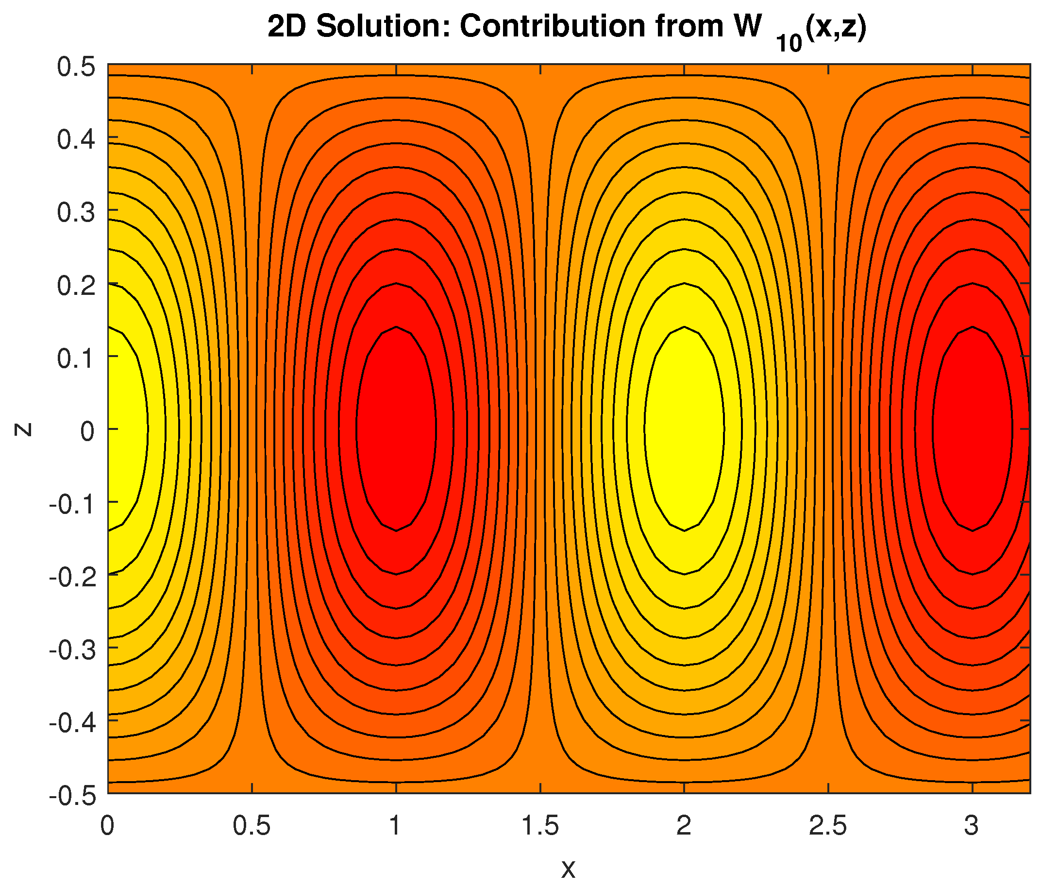
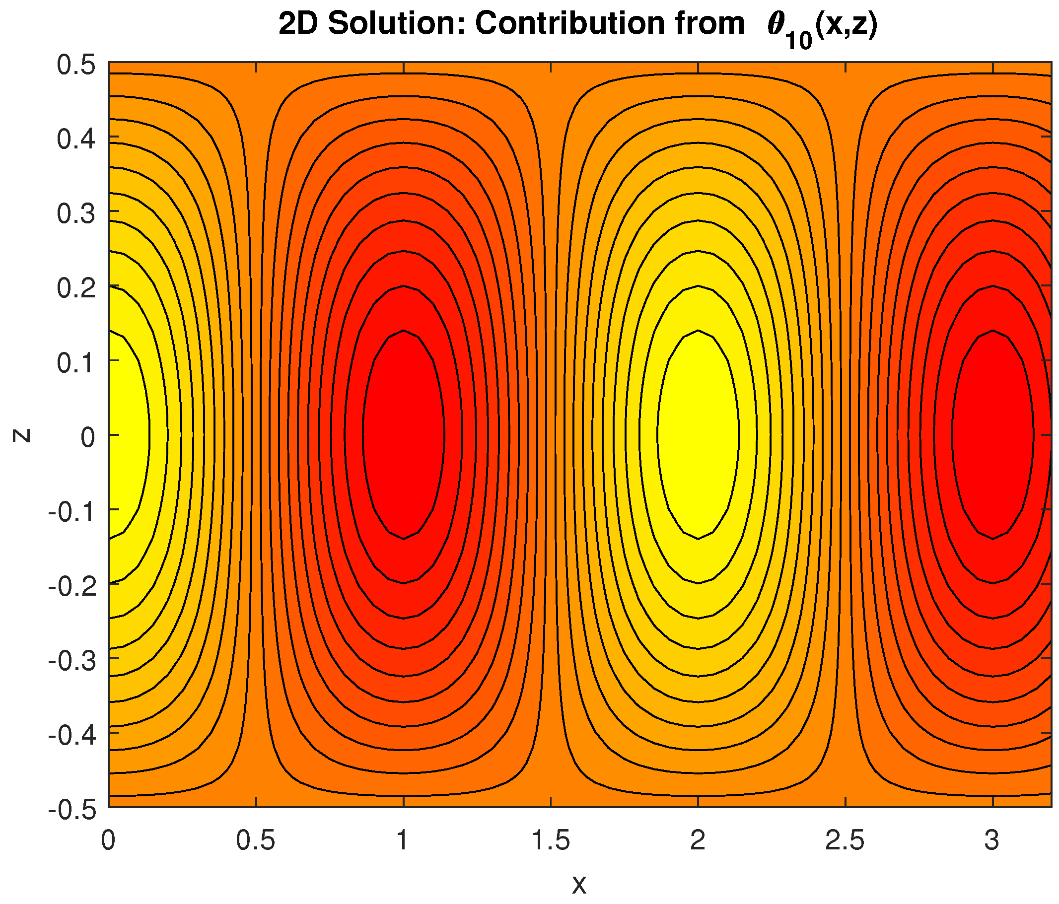
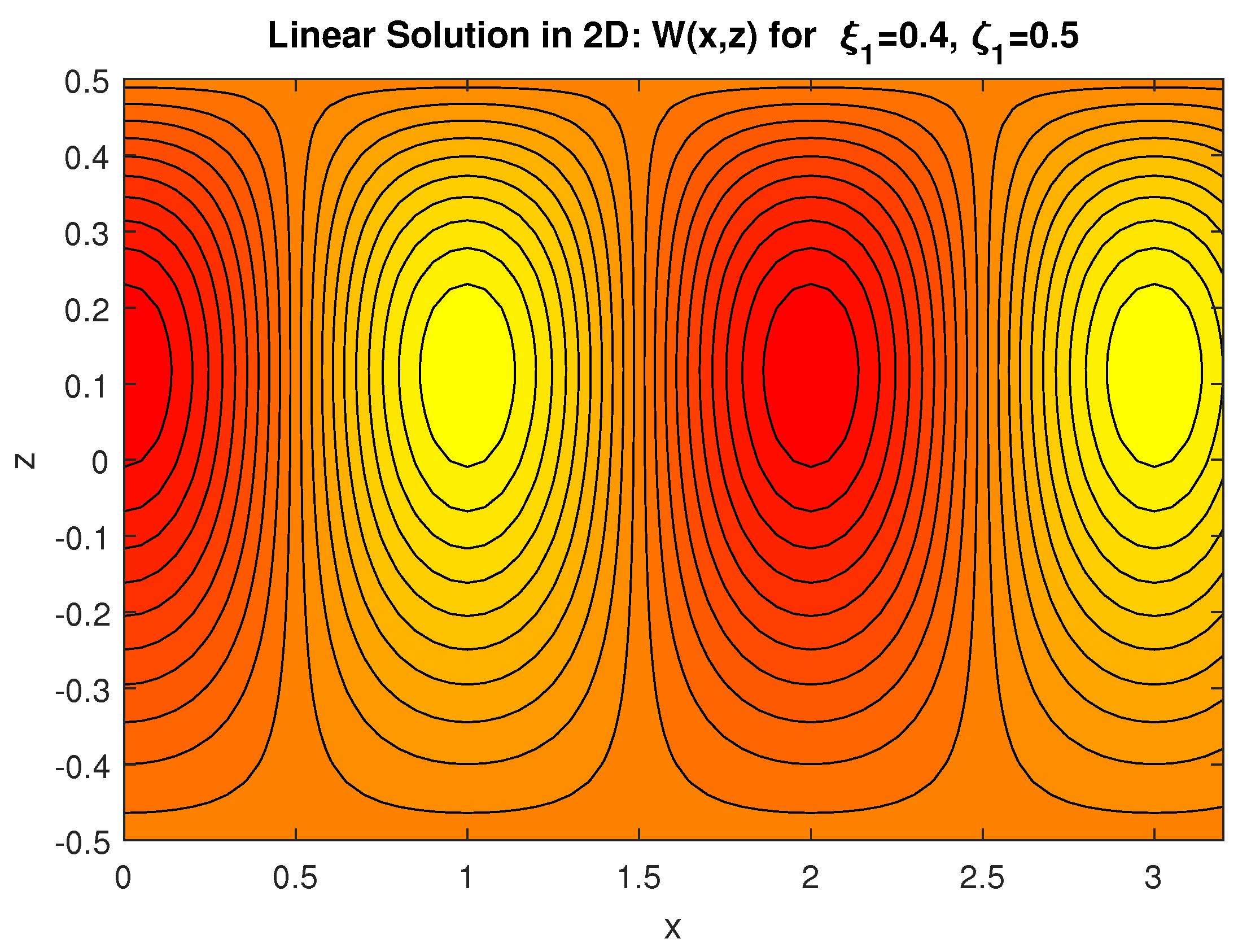
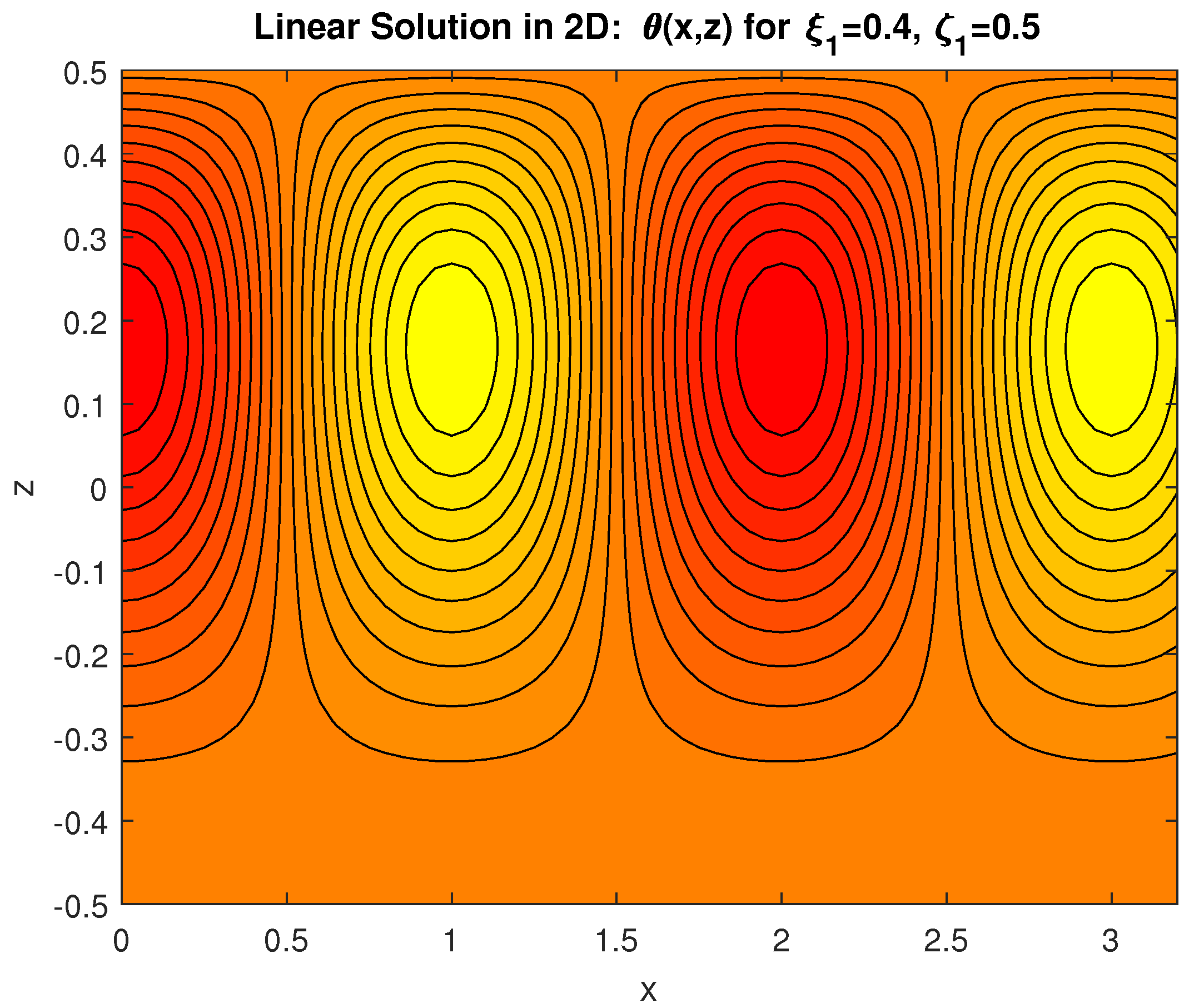
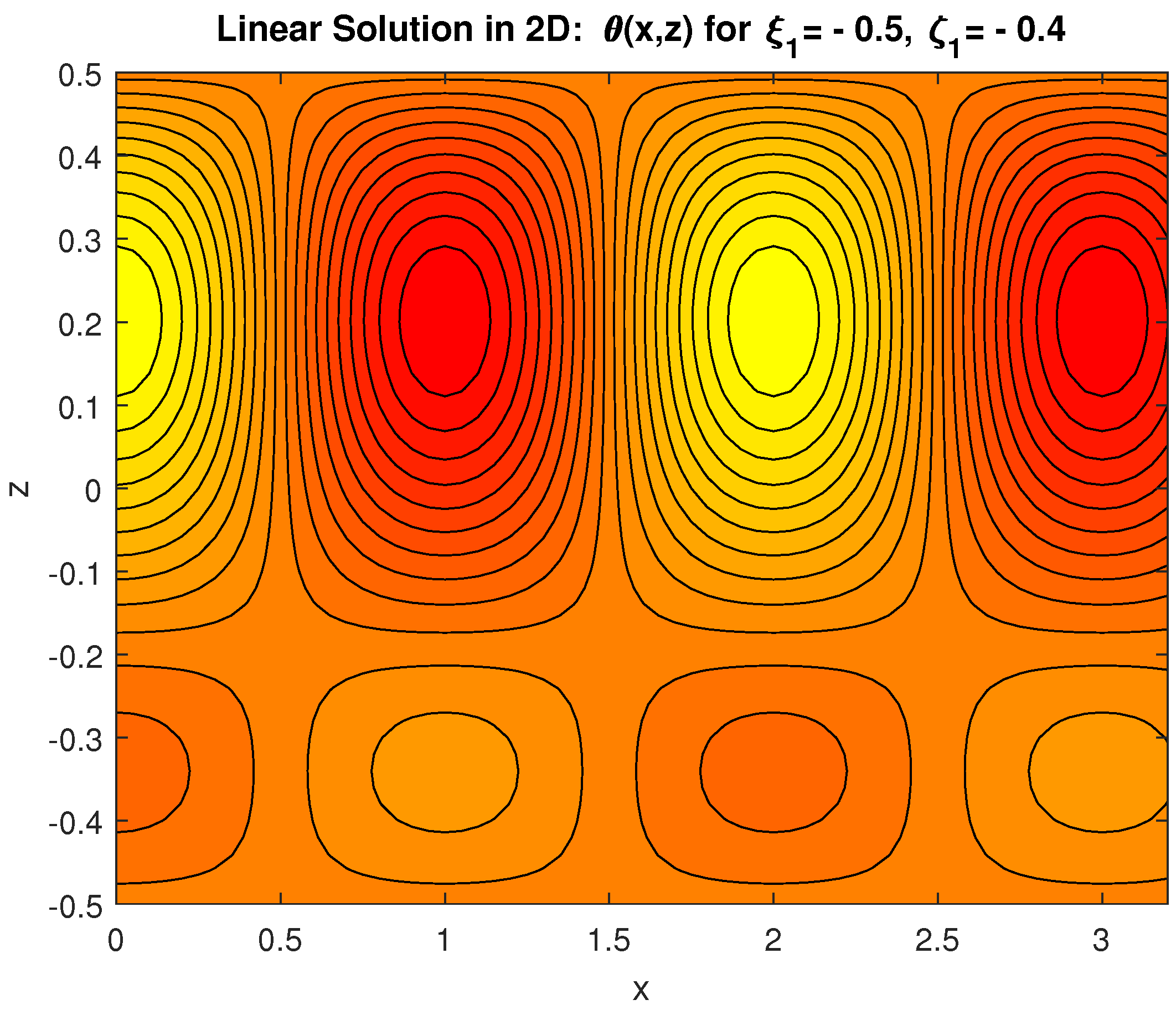
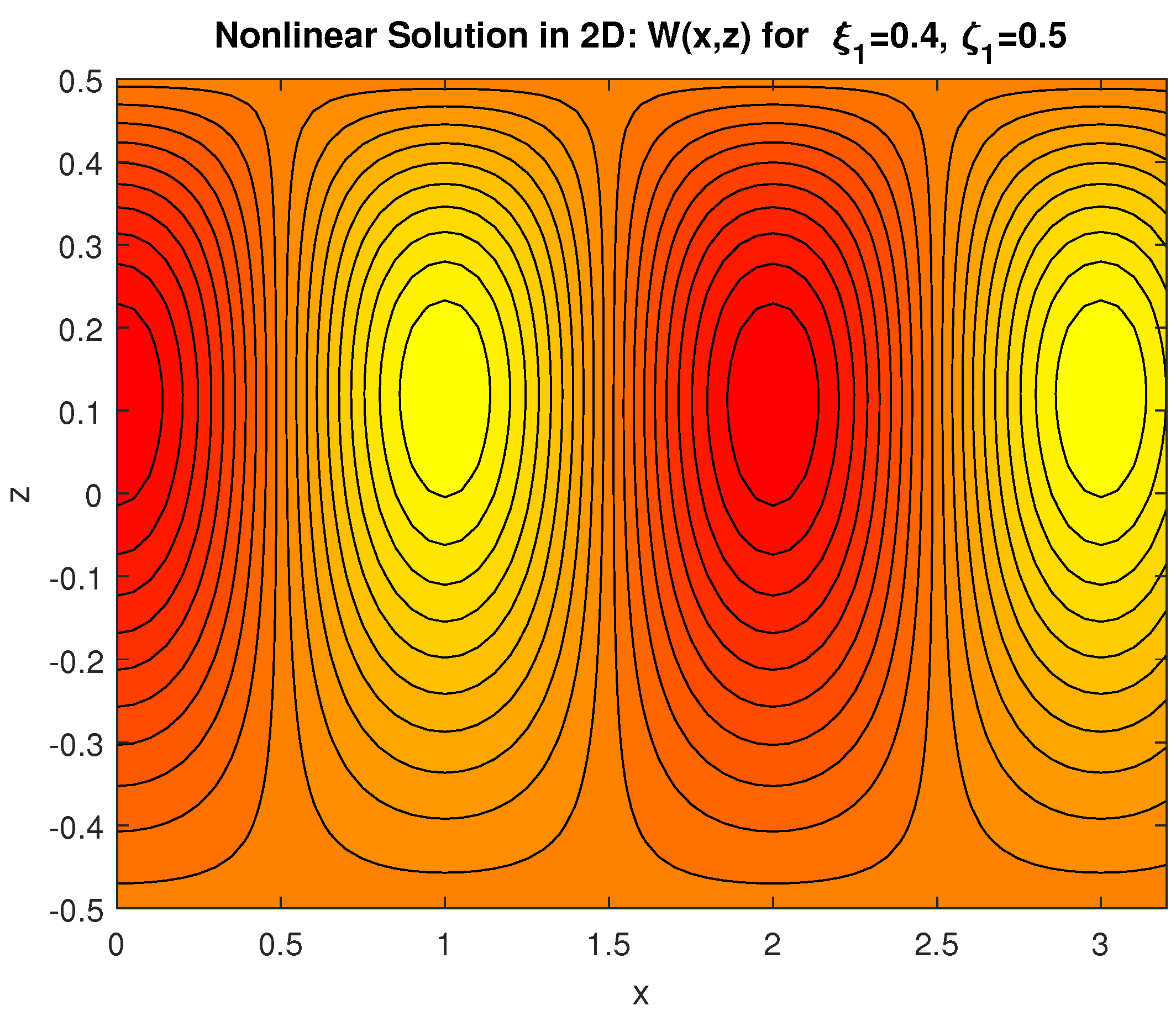
4.2. Two-Dimensional Results for $W_{10}(x.z), {\theta }_{10}(x,z), W_{11}(x,z), {\theta }_{11}(x,z), W_{20}(x,z):$

The two-dimensional zeroth order solution for $W_{10}(x,z)$ is shown in Figure 10, whereas Figure 11 displays the result for zeroth order solutions ${\theta }_{10}(x,z)$.

Two-dimensional views of flow quantities to zeroth order in $\delta$ show periodic behavior with period 2in the horizontal direction for a given z, while symmetric behavior in the vertical for a given $x$.

All the following results (Figure 12 and Figure 13) are for the parameters ${\xi }_1=0.4$ and ${\zeta }_1=0.5.$ Figure 12 presents the 2D linear solution $ϵ(W_{10}(x,z)+\delta W_{11}(x,z))$.

The linear solution $ϵ({\theta }_{10}(x,z)+\delta {\theta }_{11}(x,z))$ is shown in Figure 13.

The results presented by these two figures show the same periodicity as in Figure 10 and Figure 11, but with asymmetric behavior in the vertical for a given $x$. Similar behavior is evident in the next two Figure 14 and Figure 15.

All the following results (Figure 14 and Figure 15) are for the parameters ${\xi }_1=-0.5$ and ${\zeta }_1=-0.4.$ Figure 14 presents the 2D linear solution $ϵ\left(W_{10}(x,z)+\delta W_{11}(x,z)\right)$.

The linear solution $ϵ\left({\theta }_{10}(x,z)+\delta {\theta }_{11}(x,z)\right)$ is shown in Figure 15.

Figure 16 presents the nonlinear solutions $ϵ\left(W_{10}(x,z)+\delta W_{11}(x,z)+ϵW_{20}(x,z)\right)$ with two sets of ${\xi }_1=0.4$ and ${\zeta }_1=0.5$.

The two-dimensional profile of the nonlinear vertical velocity shows the same periodicity in the x-direction, and the vertical velocity shows slightly asymmetric behavior in the vertical direction for a given x value.

5. Conclusions

We investigated the problem of weakly nonlinear two-dimensional convective flow in a horizontal aquifer layer with horizontal isothermal and rigid boundaries. As in the application of such problems in the case of groundwater flow, we treated such a layer as a porous layer, where Darcy’s law holds, subject to the conditions that that the porous layer’s permeability and the thermal conductivity are variable in the vertical direction. The vertical axis is chosen positive in the upward direction anti-parallel to the force of gravity. In addition, our present study is restricted to the case that the subsequent hydraulic resistivity and diffusivity have small rates of change with respect to the vertical variable. We applied a weakly nonlinear approach, assuming a motionless and at most vertically-variable basic state and calculated the solutions for convective flow quantities such as vertical velocity and the temperature that arise as the Rayleigh number R exceeds its critical value $R_c$.

We found that for the case where the vertical rate of either hydraulic resistivity or diffusivity is positive, then the convective flow is stabilizing, while the flow is destabilizing when the vertical rate of such quantities is negative. The results for the flow velocity indicated that asymmetry is projected due to variations of the hydraulic resistivity or thermal diffusivity. Our results also demonstrate the presence of a non-homogeneous effect in the aquifer layer, which is known to exist due to variations in permeability and/or thermal diffusivity. The heat transported by convection increases if the vertical rate of change of either hydraulic resistivity or thermal diffusivity decreases as z increases, while the heat flux due to convection decreases if the vertical rate of change of such quantities increases as z increases.

It should be noted that the present investigation of the aquifer layer was restricted, in particular, to the two-dimensional flow case. However, the present aquifer layer problem with small variations in thermal conductivity or permeability indicated possible flow structure in the form of hexagons, which will be left as one of our future subjects of investigations. In the case of multilayer porous media, we can explore in the future the possibility of the existence of stable hexagonal cells.

References

1. Rubin, H. A note on the heat dispersion effect on thermal convection in a porous media. J. Hydrol. 1975, 25, 167–168. [Google Scholar] [CrossRef]
2. Rubin, H. Seminumerical simulation of singly dispersive convection in ground water. J. Hydrol. 1979, 40, 265–281. [Google Scholar] [CrossRef]
3. Rubin, H. Thermal convection in a nonhomogeneous aquifer. J. Hydrol. 1981, 50, 317–331. [Google Scholar] [CrossRef]
4. Riahi, D.N. Nonlinear convection in a porous layer with finite conducting boundaries. J. Fluid Mech. 1983, 129, 153–171. [Google Scholar] [CrossRef]
5. Vafai, K. Convective flow and heat transfer in variable-porosity media. J. Fluid Mech. 1984, 147, 233–259. [Google Scholar] [CrossRef]
6. Riahi, D.N. Preferred pattern of convection in a porous layer with a spatially non-uniform boundary temperature. J. Fluid Mech. 1993, 246, 529–543. [Google Scholar] [CrossRef]
7. Riahi, D.N. Modal package convection in a porous layer with boundary imperfections. J. Fluid Mech. 1996, 318, 107–128. [Google Scholar] [CrossRef]
8. Fowler, A.C. Mathematical Models in the Applied Sciences; Cambridge University Press: Cambridge, UK, 1997. [Google Scholar]
9. Bejan, A.; Khair, K.R. Heat and mass transfer by natural convection in a porous medium. Int. J. Heat Mass Transf. 1985, 28, 909–918. [Google Scholar] [CrossRef]
10. Bejan, A.; Nield, D.A. Transient forced convection near a suddenly heated plate in a porous medium. Int. Comm. Heat Mass Transf. 1991, 18, 83–91. [Google Scholar] [CrossRef]
11. Balasubramanium, R.; Thangaraj, R.P. Thermal convection in fluid layer sandwiched between two porous layers of different permeabilities. Acta Mech. 1998, 130, 81–93. [Google Scholar] [CrossRef]
12. Nield, D.A. Convection in a porous medium with inclined temperature gradient. Int. J. Heat Mass Transf. 2000, 34, 87–92. [Google Scholar] [CrossRef]
13. Nield, D.A. Some pitfall in the modelling of convective flows in porous media. Transp. Porous Media 2001, 43, 597–601. [Google Scholar] [CrossRef]
14. Rees, D.A.S. The onset of Darcy-Brinkman convection in a porous layer : an aysmptotic analysis. Int. J. Heat Mass Transf. 2002, 45, 2213–2220. [Google Scholar] [CrossRef]
15. Nield, D.A.; Bejan, A. Convection in a Porous Media, 4th ed.; Springer: New York, NY, USA, 2013. [Google Scholar]
16. Rees, D.A.S.; Pop, I. Vertical free convection in a porous medium with variable permeability effects. Int. J. Heat Mass Transf. 2000, 43, 2565–2571. [Google Scholar] [CrossRef]
17. Rees, D.A.S.; Tyvand, P.A. The Helmholtz equation for convection in two-dimensional porous cavities with conducting boundaries. J. Eng. Math. 2004, 49, 181–193. [Google Scholar] [CrossRef]
18. Rees, D.A.S.; Barletta, A. Linear instability of the isoflux Darcy-Benard problem in an inclined porous layer. Transp. Porous Media 2011, 87, 665–678. [Google Scholar] [CrossRef]
19. Rees, D.A.S.; Riley, D.S. The three-dimensional stability of finite-amplitude convection in a layered porous medium heated from below. J. Fluid Mech. 1990, 211, 437–461. [Google Scholar] [CrossRef]
20. Rees, D.A.S.; Tyvand, P.A. Onset of convection in a porous layer with continuous peridic horizontal stratification. Part I. Two-dimensional convection. Transp. Porous Media 2009, 77, 187–205. [Google Scholar] [CrossRef]
21. Bhatta, D.; Muddamallappa, M.S.; Riahi, D.N. On perturbation and marginal stability analysis of magneto-convection in active mushy layer. Transp. Porous Media 2010, 82, 385–399. [Google Scholar] [CrossRef]
22. Bhatta, D.; Riahi, D.N.; Muddamallappa, M.S. On nonlinear evolution of convective flow in an active mushy layer. J. Eng. Math. 2012, 82, 385–399. [Google Scholar] [CrossRef]
23. Bhatta, D.; Muddamallappa, M.S.; Riahi, D.N. Magnetic and permeability effects on a weakly nonlinear magneto-convective flow in active mushy layer. Int. J. Fluid Mech. Res. 2012, 39, 494–520. [Google Scholar] [CrossRef]
24. Rees, D.A.S.; Barletta, A. Onset of convection in a porous layer with continuous peridic horizontal stratification. Part II. Three-dimensional convection. Eur. J. Mech. B Fluids 2014, 47, 57–67. [Google Scholar] [CrossRef] [Green Version]
25. Anderson, D.M.; Worster, M.G. Weakly nonlinear analysis of convection in mushy layers during the solidification of binary alloy. J. Fluid Mech. 1995, 302, 307–331. [Google Scholar] [CrossRef]
Figure 1. Zeroth order solutions W 10 ( z ) .
Fluids 02 00052 g001
Figure 2. Solutions W 11 ( z ) for positive ξ 1 .
Fluids 02 00052 g002
Figure 3. Solutions θ 11 ( z ) for positive ξ 1 .
Fluids 02 00052 g003
Figure 4. Solutions W 11 ( z ) for negative ξ 1 .
Fluids 02 00052 g004
Figure 5. Solutions θ 11 ( z ) for negative ξ 1 .
Fluids 02 00052 g005
Figure 6. Linear 1D solution for W , i.e., ϵ W 10 ( z ) + δ W 11 ( z ) .
Fluids 02 00052 g006
Figure 7. Linear 1D solution for θ , i.e., ϵ θ 10 ( z ) + δ θ 11 ( z ) .
Fluids 02 00052 g007
Figure 8. Linear 1D solution for W , i.e., ϵ W 10 ( z ) + δ W 11 ( z ) .
Fluids 02 00052 g008
Figure 9. Linear 1D solution for θ i.e., ϵ θ 10 ( z ) + δ θ 11 ( z ) .
Fluids 02 00052 g009
Figure 10. Solution for W 10 ( x , z ) .
Fluids 02 00052 g010
Figure 11. Solution for θ 10 ( x , z ) .
Fluids 02 00052 g011
Figure 12. Linear 2D solution for W , i.e., ϵ W 10 ( x , z ) + δ W 11 ( x , z ) .
Fluids 02 00052 g012
Figure 13. Linear 2D solution for θ , i.e., ϵ θ 10 ( x , z ) + δ θ 11 ( x , z ) .
Fluids 02 00052 g013
Figure 14. Linear 2D solution for W , i.e., ϵ W 10 ( x , z ) + δ W 11 ( x , z ) .
Fluids 02 00052 g014
Figure 15. Linear 2D solution for θ , i.e., ϵ θ 10 ( x , z ) + δ θ 11 ( x , z ) .
Fluids 02 00052 g015
Figure 16. Nonlinear 2D solution for W , i.e., ϵ W 10 ( x , z ) + δ W 11 ( x , z ) + ϵ W 20 ( x , z ) .
Fluids 02 00052 g016