Modeling of Carbon Dioxide Leakage from Storage Aquifers

Abstract

Long-term geological storage of CO₂ in deep saline aquifers offers the possibility of sustaining access to fossil fuels while reducing emissions. However, prior to implementation, associated risks of CO₂ leakage need to be carefully addressed to ensure safety of storage. CO₂ storage takes place by several trapping mechanisms that are active on different time scales. The injected CO₂ may be trapped under an impermeable rock due to structural trapping. Over time, the contribution of capillary, solubility, and mineral trapping mechanisms come into play. Leaky faults and fractures provide pathways for CO₂ to migrate upward toward shallower depths and reduce the effectiveness of storage. Therefore, understanding the transport processes and the impact of various forces such as viscous, capillary and gravity is necessary. In this study, a mechanistic model is developed to investigate the influence of the driving forces on CO₂ migration through a water saturated leakage pathway. The developed numerical model is used to determine leakage characteristics for different rock formations from a potential CO₂ storage site in central Alberta, Canada. The model allows for preliminary analysis of CO₂ leakage and finds applications in screening and site selection for geological storage of CO₂ in deep saline aquifers.

1. Introduction

It is generally accepted that increase in concentrations of greenhouse gases (GHG) such as carbon dioxide (CO₂), methane (CH₄) and nitrous oxide (N₂O) is the main cause of global warming [1]. It has been reported that the anthropogenic emissions have increased atmospheric concentrations of CO₂ by around 35% during the last 200 years, from 280 ppm in 1800 to 380 ppm in 2005 [1]. The rate of anthropogenic emissions to the atmosphere is also continuing to increase. In 1950, anthropogenic emissions of CO₂ were around 6 Gt of CO₂; in 2000, this number was around 22 Gt CO₂/year; and in 2015 the number was estimated to be approximately 37 Gt CO₂/year [2]. From this amount, approximately 45% of the emitted anthropogenic carbon remains in the atmosphere, and the other 55% goes into the ocean and land biomass [2]. Therefore, to mitigate the effects on climate change, CO₂ emissions to the atmosphere should be reduced, and the concentration of CO₂ needs to be stabilized at around 450 ppm by 2050 [1]. One attractive option for reducing CO₂ emissions is carbon capture and storage (CCS) [1]. CCS involves capturing CO₂ from energy related sources such as large industrial plants, transporting it to a suitable storage location and storing it in deep geological formations, before it is emitted to the atmosphere.

Among the proposed CCS options, sequestration in deep saline aquifers appears to be the most promising option due to the relatively larger storage capacity and worldwide distribution of these formations [1]. Deep saline aquifers are permeable layers (usually found in sedimentary basins), saturated with salt water and bounded from below and above by less permeable rocks. Proper analysis of CO₂ storage in deep saline aquifers requires understanding of the properties of carbon dioxide and other fluids involved in the system, as well as properties of the geological formations. For temperatures greater than T_c = 31.1 °C and pressures greater than P_c = 7.38 MPa (critical point), CO₂ is in the supercritical state. The depth of CO₂ injection in sedimentary basins is usually considered sufficiently deep to maintain the CO₂ in a supercritical state.

Trapping of carbon dioxide in saline aquifers can be broadly classified into structural/stratigraphic, residual, solubility, and mineral trapping mechanisms. Structural/stratigraphic trapping refers to the processes in which CO₂ is trapped in free phase under a geological structure such as an impermeable layer [3]. In this case, CO₂ could be mobile but trapped since an impermeable layer prevents upward migration of CO₂. In residual trapping, CO₂ is stored as an immobile phase due to capillary forces and relative permeability hysteresis. In a longer period of time, solubility and mineral trapping contribute in reduction of the free phase CO₂. Carbon dioxide storage is likely secure in the cases of residual trapping as well as mineral and dissolution trapping. However, in the case where CO₂ is in structural/stratigraphic traps, buoyancy will always act to drive free and mobile CO₂ upward and, if CO₂ encounters a high permeable pathway, it will leak into the overlying formation (e.g., shallower groundwater or atmosphere) which might cause serious environmental impacts such as contamination of groundwater resources used for agricultural, industrial or human consumption, or might be a risk to vegetation, animal and human life [1].

Two approaches are commonly considered to study sequestration processes. The first approach involves long-term (century-to-millennium) processes such as dissolution of CO₂ in the aquifer brine and geochemical mineralization of CO₂. These studies focus on the convective dissolution and mineral trapping of carbon dioxide. Emami-Meybodi et al. [4] provided a complete review of convective mixing as a result of CO₂ dissolution at the interface between the CO₂ plume and the underlying brine. The second approach involves short time scales (during injection and shortly after CO₂ injection is ceased) and uses the principles of two-phase flow in porous media. It considers supercritical CO₂ and brine as two immiscible fluid phases, which can be described by relative permeability and capillary pressure relationships. In this study, we focus on the second approach and ignore the dissolution to investigate the processes and driving forces that are active on relatively short time scales after CO₂ injection.

Migration of a buoyant fluid in a porous medium as a gravity current has received considerable attention for quite some time. In an early study, Bear [5] derived a sharp interface model for displacement of one fluid by another fluid with different densities and viscosities in a tilted confined porous layer, with background flow. More recently, Nordbotten et al. [6] studied the injection of CO₂ into a saline aquifer and derived an analytical solution for evolution of CO₂ plume during injection through a single well, into a horizontal and homogeneous aquifer. They defined a gravity number that expresses the ratio of buoyancy to viscous forces as $2\pi \Delta \rho gk{\lambda }_w{H}^2/Q$, where $\Delta \rho$ is the density difference between formation brine and CO₂ at in-situ condition, $k$ is the aquifer permeability, ${\lambda }_w$ is brine mobility (defined as ${\lambda }_w=k_{rw}/{\mu }_w$) and $H$ and $Q$ are aquifer thickness and injection rate at the in-situ condition. Other analytical solutions are available in the literature which describe the evolution of supercritical CO₂ plume during injection into deep saline aquifers [7,8,9]. Depending on the parameters used in non-dimensionalizing the flow equations, different expressions for gravity number can be derived. For example, Ide et al. [10] used another expression for gravity number to define ratio of gravity to viscous forces as $k_{\mathrm{v}}L\Delta \rho g/Hu{\mu }_w$, where $k_{\mathrm{v}}$ is vertical permeability, $L$ is the aquifer length and $u$ is the total average Darcy velocity. They performed simulations to study immobilization of CO₂ plume by capillary trapping and concluded that the amount of injected CO₂ that can be immobilized by residual trapping is a strong function of the gravity number, where the total amount of the trapped gas decreases as gravity number increases. They also showed that capillary pressure and aquifer tilt angle affect the value and the rate of trapping.

Kopp et al. [11,12] through dimensional analysis showed that the balance between driving forces control the displacement of CO₂ plume in an aquifer during CO₂ injection. They reported dimensionless gravitational and capillary numbers and examined their effects on storage capacity of reservoirs. They showed that a low ratio of gravitational to viscous forces (low gravitational number) and to a lesser extent a high ratio of capillary to viscous forces (high capillary number) leads to a higher CO₂ storage capacity.

Possible leakage pathways could be in the form of natural interruptions and breaches through the confining strata such as open faults, fractures and erosional channels, or they could be in the form of manmade or artificial pathways such as abandoned wells or activated faults and fractures [13,14].

Figure 1 shows pathways for CO₂ migration for a possible leakage. Inactive faults can be reactivated because of local pressure changes during CO₂ injection. Likewise, closed fractures may open by exceeding bottom hole pressure from the minimum in-situ stress. There is an active debate on whether injection of CO₂ will trigger large earthquakes and reactivate faults and therefore threaten the seal integrity of CO₂ storage reservoirs [15,16]. The main geomechanical aspects affecting the integrity of the CO₂ storage sites have been reviewed by different researchers [17,18]. For large scale injection operations, domains in the order of thousands of square kilometers need to be analyzed to guarantee the safety of storage [19].

Leakage of CO₂ can be assessed by means of numerical and analytical models. Analytical solutions can only be derived with sufficient restrictive assumptions. Various analytical solutions have been published in the literature, especially for the leakage along existing wells [20,21,22]. Additionally, theoretical models are developed for investigating diffusive leakage of brine from an aquifer into overburden and underburden formations during geological storage of CO₂ [23,24]. Although several efforts have been devoted to assess the risk of leakage through existing wells, leakage through faults and fractures has been less addressed in the literature, and it is partly due to the difficulty in characterizing the features of such pathways. Useful numerical simulations for CO₂ leakage through existing/activated faults have been published in the literature [25,26,27,28]. Recently, Kang et al. [29] used a simplified model to derive expressions for pressure drawdown and interface upconing around a leaky fault. They described a vertical two-phase flow along a fault and concluded that, for estimation of leakage, structures and properties of the fault must be included in the model.

Even with large potential capacity of saline aquifers, a major obstacle to implement CO₂ sequestration in such formations is the lack of insights into the risks associated with it. In relatively short time scales, CO₂ injected into saline aquifer is in free phase and prone to leakage. Therefore, for selection of storage sites, it is important to know, in case of a leaky fault or fracture, how much CO₂ will leak and how long it will take to happen. The combined effect of different mechanisms and their evolution with time and space can only be evaluated through sophisticated numerical simulations. The objective of this paper is to develop a simple model which allows for quick and relatively easy screening of storage reservoirs by investigating processes and driving forces that are active on CO₂ plume in relatively short time scales after CO₂ injection.

2. Model Description and Governing Equations

To study migration of CO₂ along a water-saturated fault zone, a one-dimensional (1D) model is developed. To provide conservative estimates of the leakage potential, we ignore the effect of dissolution trapping and the system is assumed to be isothermal.

CO₂ (non-wetting phase) and formation brine (wetting phase) are assumed to be immiscible and the interphase transfer between phases (mass transfer between the fluids, i.e., dissolution of CO₂ in brine and evaporation of brine into CO₂) is neglected.

Mass conservation equation and the extended Darcy formula are the governing equations of two immiscible fluids flow in porous layer for a linear system which can be written separately for each phase. The modified Darcy’s law for multi-phase flow, which relates the volumetric flux of each phase to the respective phase pressure, can be written as [5]:

$${\overrightarrow{\mathbf{v}}}_{\alpha }=-\frac{k{k}_{r\alpha }}{{\mu }_{\alpha }}\left(\nabla p_{\alpha }+{\rho }_{\alpha }g\nabla z\right)=-k{\lambda }_{\alpha }\left(\nabla p_{\alpha }+{\rho }_{\alpha }g\nabla z\right)\alpha =w,nw$$

(1)

where ${\overrightarrow{\mathbf{v}}}_{\alpha }$ is the Darcy velocity [${\mathrm{LT}}^{-1}$] of phase $\alpha$, $k$ is the absolute (intrinsic) permeability [${\mathrm{L}}^2$] of the formation, $k_{r\alpha }$ is the relative permeability of phase $\alpha$, ${\mu }_{\alpha }$ is the viscosity [${\mathrm{ML}}^{-1}{\mathrm{T}}^{-1}$] of phase $\alpha$, $p_{\alpha }$ is the pressure [${\mathrm{ML}}^{-1}{\mathrm{T}}^{-2}$] of phase $\alpha$, ${\rho }_{\alpha }$ is the density [${\mathrm{ML}}^{-3}$] of phase $\alpha$, $g$ is the gravitational [${\mathrm{LT}}^{-2}$] acceleration, $z$ is the vertical coordinate [$\mathrm{L}$] and positive upward, and ${\lambda }_{\alpha }=k_{r\alpha }^{}/{\mu }_{\alpha }$ is the mobility of phase $\alpha$.

Mass balance equation for each phase is given by [5]:

$$\frac{\partial (\varphi {\rho }_{\alpha }{S}_{\alpha })}{\partial t}+\nabla ·({\rho }_{\alpha }{\overrightarrow{\mathbf{v}}}_{\alpha })-{\rho }_{\alpha }{q}_{\alpha }=0\alpha =w,nw$$

(2)

where $\varphi$ is formation porosity and $q_{\alpha }$ represents source/sink term [${\mathrm{T}}^{-1}$]. By substitution of Equation (1) into Equation (2), a system of partial differential equations is obtained for each phase.

Additional closure equations are required to solve the system of the partial differential equations. First, the sum of phase saturations equals unity.

$${\displaystyle \sum _{\alpha }{S}_{\alpha }}=1$$

(3)

Second, the pressure difference between the two phases equals capillary pressure $p_c$ [5]:

$$p_c=p_{nw}-p_w$$

(4)

Finally, to solve the system of partial differential equations, constitutive relations are required, which include capillary pressure and relative permeability as functions of saturation. In this study, the following assumptions have been made to simplify the modeling of two-phase flow. The porous layer (leakage pathway) is considered homogenous, isotropic and one-dimensional tilted with an angle $\theta$ from the horizontal axis. Formation brine ($w$) and gas/supercritical phase ($nw$) are single-component fluids and are assumed to be incompressible. The flow is considered isothermal, sources and sinks are not present and the dynamic viscosity is also assumed to be constant. These assumptions allow development of a simple and fast model for analysis of leakage and have been previously used in many studies. Nevertheless, modeling of CO₂ leakage from leakage pathways in the absence of these assumptions requires detailed geological and numerical models. Simulation of CO₂ leakage including all details, such as 3D features, pathway heterogeneities, phase behavior and phase change, geomechanical effects, thermal, and geochemical effects, is very time consuming and difficult, if not impossible. In addition, simple models often provide a first order estimate of CO₂ leakage necessary for site screening and risk assessment. A schematic of the problem is shown in Figure 2.

Using the above-mentioned assumptions and adding the definition of capillary pressure (Equation (4)), CO₂ flux can be written as:

$${\mathbf{v}}_{nw}=\frac{k{\lambda }_{nw}{\lambda }_w}{{\lambda }_t}\left[-\frac{d{p}_c}{d{S}_{nw}}\frac{\partial S_{nw}}{\partial z}+\Delta \rho g\sin \theta \right]+\frac{{\lambda }_{nw}{\mathbf{v}}_t}{{\lambda }_t}$$

(5)

With substitution in mass balance equation, saturation equation for CO₂ phase can be written as:

$$\varphi \frac{\partial S_{nw}^{}}{\partial t}+\frac{\partial }{\partial z}\left[-\frac{k{\lambda }_{nw}{\lambda }_w}{{\lambda }_t}\frac{d{p}_c}{d{S}_{nw}}\frac{\partial S_{nw}}{\partial z}+\frac{k{\lambda }_{nw}{\lambda }_w}{{\lambda }_t}\Delta \rho g\sin \theta +\frac{{\lambda }_{nw}}{{\lambda }_t}{\mathbf{v}}_t\right]=0$$

(6)

where ${\mathbf{v}}_t={\mathbf{v}}_{nw}+{\mathbf{v}}_w$ is constant total velocity and is defined as the summation of CO₂ and brine velocities. In addition, ${\lambda }_t={\lambda }_{nw}+{\lambda }_w$ and $\Delta \rho ={\rho }_w-{\rho }_{nw}$ are total mobility and density difference, respectively.

Equation (6) is a second-order nonlinear partial differential equation, which is of the general form for describing flow of two immiscible incompressible fluids in a one-dimensional porous media. To develop the dimensionless form of Equation (6), the following dimensionless variables are defined.

$$S=\frac{S_{nw}-S_{cc}}{1-S_{wr}-S_{cc}}$$

(7)

$$z_D=\frac{z}{l_{cr}}$$

(8)

$$t_D=\frac{t}{t_{cr}}$$

(9)

$$t_{cr}=\frac{{\varphi }^{*}{l}_{cr}}{{\mathbf{v}}_t}$$

(10)

where ${\varphi }^{*}=\varphi (1-S_{wr}-S_{cc})$.

In the above equations, $S$ is the normalized gas saturation varying between 0 and 1, $S_{wr}$ is the irreducible (or residual) saturation of brine, and $S_{cc}$ is the critical gas saturation. Fluid saturations are often normalized with respect to the ranges of values occurring in the problem under consideration. $1-S_{wr}$ and $S_{cc}$ are the maximum and minimum saturations that occur during the migration of CO₂, respectively. Dimensionless variables $z_D$ and $t_D$ are dimensionless length and time ($0\le z_D\le 1$, $t_D\ge 0$), respectively. Parameters $l_{cr}$ and $t_{cr}$ are the characteristic values for length and time, respectively. Choosing the correct characteristic scale is of great importance and requires a well-developed understanding of the system being analyzed since it can change the dimensionless numbers (see Section 3.1) by orders of magnitudes [11]. In this study, the total length of the system is used to scale the migration length ($l_{cr}=L$) and $t_{cr}$ is the time at which the migrating CO₂ travels the length of the system by pure advection.

With substitutions, the dimensionless velocity of CO₂ (${\mathbf{v}}_D$) is obtained as:

$${\mathbf{v}}_D=\frac{{\mathbf{v}}_{nw}}{{\mathbf{v}}_t}=-\frac{k{\lambda }_{nw}{\lambda }_w}{L{\mathbf{v}}_t{\lambda }_t}\frac{d{p}_c}{dS}\frac{\partial S}{\partial z_D}+\frac{k{\lambda }_{nw}{\lambda }_w}{{\mathbf{v}}_t{\lambda }_t}\Delta \rho g\sin \theta +\frac{{\lambda }_{nw}}{{\lambda }_t}$$

(11)

and the gas saturation equation (Equation (6)) therefore can be written as:

$$\frac{\partial S}{\partial t_D}+\frac{\partial }{\partial t_D}\left(-\frac{k{\lambda }_{nw}{\lambda }_w}{L{\mathbf{v}}_t{\lambda }_t}\frac{d{p}_c}{dS}\frac{\partial S}{\partial z_D}+\frac{k{\lambda }_{nw}{\lambda }_w}{{\mathbf{v}}_t{\lambda }_t}\Delta \rho g\sin \theta +\frac{{\lambda }_{nw}}{{\lambda }_t}\right)=0$$

(12)

To determine solution of Equation (12), proper saturation functions for capillary pressure and relative permeability are required. In this study, the following relative permeability relations as function of saturation are used in the form of Brooks-Corey equation [30].

$$k_{rnw}^{}=k_{rnw}^{\max }{(S)}^{nc}$$

(13)

$$k_{rw}^{}=k_{rw}^{\max }{(1-S)}^{nb}$$

(14)

In the above equation, $k_{rnw}^{\max }$ is the relative permeability of CO₂ at irreducible brine saturation, and $k_{rw}^{\max }$ is the relative permeability to brine at the critical CO₂ saturation. For the drainage cycle, $k_{rw}^{\max }=1$ and $S_{cc}^{}=0$. Parameters nc and nb are the constants (also known as Corey’s coefficients), which affect the shape of the relative permeability curves. Increasing values of these coefficients cause the relative permeability curve to become concave. The capillary pressure is represented by a logarithmic function, which has been conventionally used for such problems [31].

$$p_c=-p_d^{}\ln (1-S)$$

(15)

where $p_d$ is the capillary entry pressure.

Different dimensionless numbers can be established to define the balance between driving forces taking place during and after CO₂ injection. For the CO₂ injection application, Kopp et al. [11] used dimensionless capillary and gravitational numbers and qualitatively examined their effects on storage capacity. Here, we use a similar form of dimensionless numbers for our system.

Substitution of Equations (13)–(15) into Equations (11) and (12) gives:

$${\mathbf{v}}_D=\underset{{\mathbf{v}}_{DD}}{\underbrace{-N_{Ca}D(S)\frac{\partial S}{\partial z_D}}}+\underset{{\mathbf{v}}_{DG}}{\underbrace{N_{Gr}G(S)}}+\underset{{\mathbf{v}}_{DV}}{\underbrace{V(S)}}$$

(16)

$$\frac{\partial S}{\partial t_D}+\frac{\partial }{\partial z_D}\left[-N_{Ca}D(S)\frac{\partial S}{\partial z_D}+N_{Gr}G(S)+V(S)\right]=0$$

(17)

where ${\mathbf{v}}_{DD}$, ${\mathbf{v}}_{DG}$ and ${\mathbf{v}}_{DV}$ are capillary, gravity and viscous contribution to dimensionless CO₂ velocity, respectively. $N_{Ca}$ is the dimensionless capillary number and $N_{Gr}$ is the dimensionless gravity number, which relate forces acting on the system and are analyzed based on the reservoir parameters as well as fluid properties as follow.

$$N_{Ca}=\frac{k{k}_{rnw}^{\max }{p}_d}{L{\mu }_{nw}{\mathbf{v}}_t}\frac{\mathrm{Capillary}\mathrm{Forces}}{\mathrm{Viscous}\mathrm{Forces}}$$

(18)

$$N_{Gr}=\frac{k{k}_{rnw}^{\max }\Delta \rho g\sin \theta }{{\mu }_{nw}{\mathbf{v}}_t}\frac{\mathrm{Gravity}\mathrm{Forces}}{\mathrm{Viscous}\mathrm{Forces}}$$

(19)

$D(S)$, $G(S)$ and $V(S)$ are capillary, gravity and viscous functions, respectively, and are defined as:

$$D(S)=\frac{S^{nc}{\left(1-S\right)}^{nb-1}}{M{S}^{nc}+{(1-S)}^{nb}}\mathrm{Capillary}\mathrm{Function}$$

(20)

$$G(S)=\frac{{(S)}^{nc}{(1-S)}^{nb}}{M{(S)}^{nc}+{(1-S)}^{nb}}\mathrm{Gravity}\mathrm{Function}$$

(21)

$$V(S)=\frac{M{(S)}^{nc}}{M{(S)}^{nc}+{(1-S)}^{nb}}\mathrm{Viscous}\mathrm{Function}$$

(22)

where

$$M=\frac{k_{rnw}^{\max }/{\mu }_{nw}}{k_{rw}^{\max }/{\mu }_w}\mathrm{Mobility}\mathrm{Ratio}$$

(23)

Equation (17) is used to simulate CO₂ migration in a linear porous media and considers viscous, capillary and gravity forces simultaneously. Equation (17) is a nonlinear second order partial differential equation, which is also known as nonlinear convection–diffusion equation. A similar form of this equation has been developed before for the application of water flooding in oil reservoirs [32]. The first term in Equation (17) is the accumulation term; the second term includes the contribution of capillary forces in the displacement process and has a diffusive nature; the third term contains the gravitational contributions to the flow and has an advective character; and the fourth term is the contribution of viscous forces and same as the third term has an advective character.

The problem described by Equation (17) is completed by setting proper initial and boundary conditions. In this study, we assume that the entire domain is initially fully saturated with brine, therefore only primary drainage process is considered here, and the residual CO₂ is not a concern. At the inlet boundary, it is considered that CO₂ saturation is always at its maximum value. This assumption seems reasonable when CO₂ has already displaced the formation brine beneath a leakage pathway and a residual saturation of the wetting phase has been established. At the outlet boundary it is assumed that the changes in CO₂ saturation is negligible. This boundary condition infers negligible diffusive (capillary) flux at the outer boundary compared to gravity and viscous fluxes. The initial and boundary conditions are then given by:

$$t_D=0S=0$$

(24)

$$z_D=0S=1$$

(25)

$$z_D=1\frac{\partial S}{\partial z_D}=0$$

(26)

The model described above forms the basis of this study. Numerical discretization and detailed validation of the developed model is presented in Appendix A and Appendix B, respectively.

3. Results and Discussion

The developed model in the previous section is utilized to understand processes and driving forces active during leakage of CO₂ into the shallower formations. This section is organized as follows. First, the effect of dimensionless numbers and interaction of forces on the displacement process and leakage is investigated. Next, the developed model is used to assess leakage in seven formations located in Alberta, Canada, which are considered potential options for geological storage of CO₂.

3.1. Interaction of Gravity, Capillary, and Viscous Forces

To investigate the effect of forces acting on the fluid flow and rate of leakage, we define seven different datasets. Detailed comparison and properties of each set is presented in

Table 1. Simulation parameters used in qualitative analysis.

Data	Dataset 1	Dataset 2	Dataset 3	Dataset 4	Dataset 5	Dataset 6	Dataset 7
Capillary entry pressure, $p_d$ (MPa)	0.2	1.5	0.2	0.2	0.2	0.2	0.2
Tilt angle, $\theta$	π/23	π/23	π/2	π/23	π/23	π/23	π/23
Total velocity, ${\mathbf{v}}_t$ (m/s)	3 × 10−6	3 × 10−6	3 × 10−6	3 × 10−7	3 × 10−6	3 × 10−6	3 × 10−6
End-point rel-perm of CO2, $k_{rnw}^{\max }$	0.65	0.65	0.65	0.65	0.065	0.65	0.65
Corey Exponent for Brine, $nb$	2	2	2	2	2	4	2
Corey exponent for CO2, $nc$	2	2	2	2	2	2	4
$M$	10.03	10.03	10.03	10.03	1.00	10.03	10.03
$N_{Ca}$	0.155	1.161	0.155	1.548	0.015	0.155	0.155
$N_{Gr}$	0.155	0.155	1.139	1.550	0.016	0.155	0.155

. The following properties are assumed to be the same for all the seven datasets. Length of the domain ($L$) is considered to be 500 m. Density difference between CO₂ and brine ($\Delta \rho ={\rho }_w-{\rho }_{nw}$) is assumed to be 300 kg/m³ and porosity ($\varphi$) is 0.2. Brine and CO₂ viscosity are assumed to be 0.86 and 0.06 mPa·s, respectively. Absolute permeability is taken to be 100 mD and residual water saturation ($S_{wr}$) is assumed to be 0.3. Parameters used for these datasets are only for comparison and they are not related to a specific reservoir. The last three rows in Table 1 show the calculated mobility ratio, $N_{Ca}$ and $N_{Gr}$. Dataset 1 is considered as base case. In each dataset, the changing parameter is bolded in Table 1. Two analysis groups have been established. First, the effect of changes in $N_{Ca}$ and $N_{Gr}$ is investigated, while $D(S)$, $G(S)$ and $V(S)$ are kept constant (Datasets 2–4). Second, changes of relative permeability parameters of CO₂ and brine system are examined, which include the effect of mobility ratio and Corey exponents nb and nc (Datasets 5–7). Changes in gas saturation profile and gas dimensionless velocity are examined for each dataset. Breakthrough time is considered to be the time when migrating CO₂ appears at the outlet boundary.

Figure 3 shows the parameters map of $N_{Gr}-N_{Ca}$ space. A reference equilibrium state between gravitational and viscous forces is indicated with dotted line at $N_{Gr}=1$ and between capillary and viscous forces at $N_{Ca}=1$. In Figure 3, the lower left sector represents domination of viscous forces over capillary and gravitational forces. As we move from this sector to the right or top, viscous forces lose their influence in favor of capillary (lower right sector) or gravitational (upper left sector) forces, respectively. Finally, in the upper right sector, capillary and gravitational forces dominate over viscous forces.

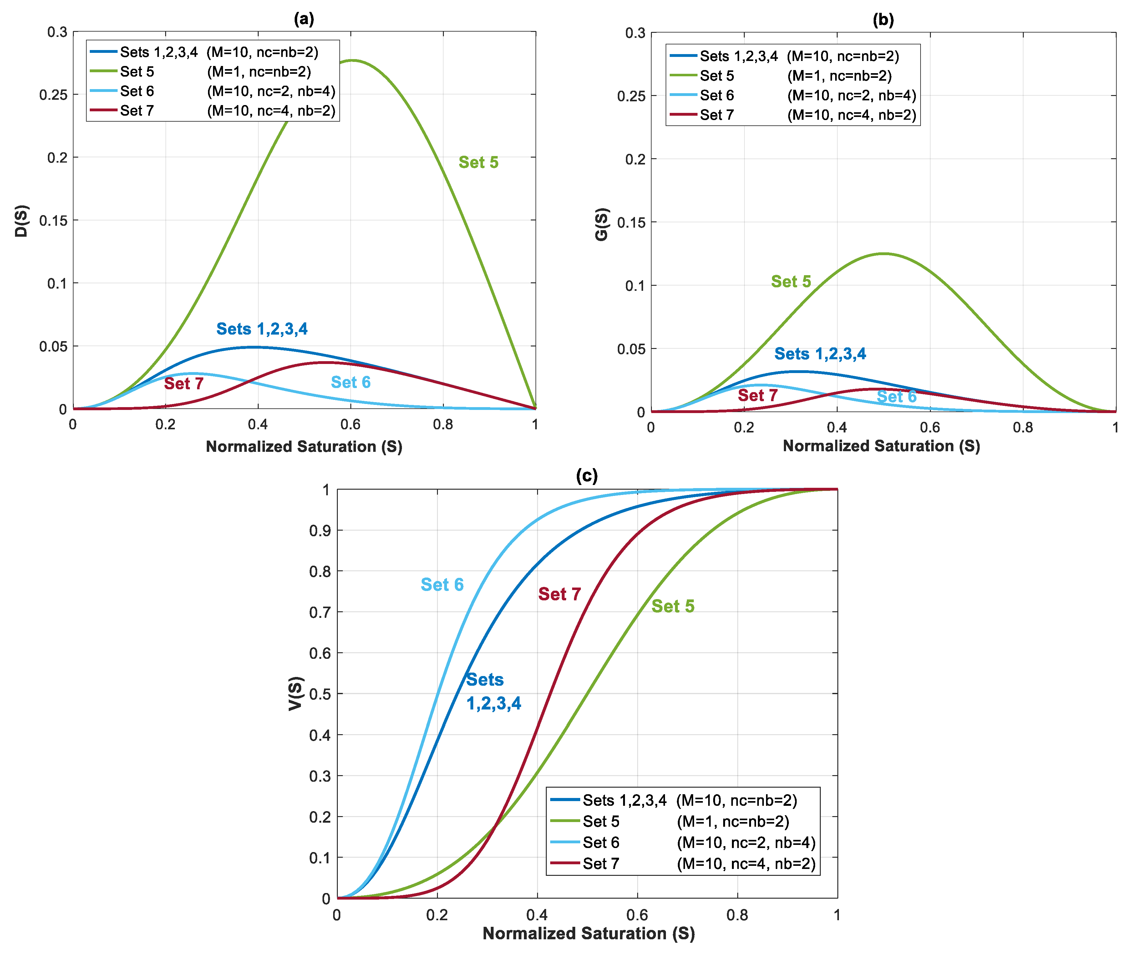
Capillary, gravity and viscous functions are plotted for all seven datasets in Figure 4a–c. The shape and value of these functions are influenced by Corey exponents in relative permeability equation (nc and nb), and mobility ratio. Capillary function $D(S)$ (Figure 4a) and gravity function $G(S)$ (Figure 4b) have a bell shape, whereas shape of $V(S)$ is the same as the fractional flow equation in Buckley–Leveret problem.

In the first four datasets, dimensionless functions $D(S)$, $G(S)$ and $V(S)$ are same. In Datasets 5–7, relative permeability parameters are changed to evaluate their effect on flow process. Migration of CO₂ plume depends on balance of these forces, which determines the security of storage.

Figure 5 shows the normalized gas saturation and contribution of different forces in CO₂ dimensionless velocity versus dimensionless length at time $t_D=0.2$ for Datasets 1 to 4.

For Dataset 1 (Table 1), $N_{Ca}$ and $N_{Gr}$ have the same magnitude and less than one, and position of this dataset in the parameter space map is in the lower left sector of Figure 3. This is translated to dominance of viscous forces over capillary and gravity forces. As shown in Figure 5, higher viscous forces lead to a CO₂ plume with sharp front. As a result, plume migration is slowest among other datasets (Datasets 2–4). In this case, gravitational forces are rather weak, leading to a low buoyancy-induced upward migration of CO₂.

In Dataset 2, the effect of capillary entry pressure, $p_d$, is investigated. By changing the capillary entry pressure ($p_d$) from 0.2 MPa to 1.5 MPa, capillary number ($N_{Ca}$) increases up to 1.161, while the gravity number ($N_{Gr}$) remains the same as the one used in Dataset 1. This leads to a shift to the lower right corner of the parameter map, as shown in Figure 3. Increasing capillary number will increase the influence of capillary forces over viscous forces. Stronger capillary forces lead to a more diffusive-like front propagation. An earlier breakthrough is a result of higher capillary forces, as shown in the saturation distributions and velocity profiles for Datasets 1 and 2 in Figure 5a,b (and later in Figure 6a). As shown in Figure 5c, as $N_{Ca}$ increases in Dataset 2, contributions of capillary forces on CO₂ plume velocity (${\mathbf{v}}_{DD}$) increases. As the effect of capillary forces increases, the inlet dimensionless velocity (${\mathbf{v}}_D$) of the migrating CO₂ takes values greater than one. This is because the dimensionless velocity of the migrating CO₂ is given by ${\mathbf{v}}_D=1-{\mathbf{v}}_b/{\mathbf{v}}_t$. At high capillary forces, there is backward flow of brine as CO₂ migrates upward. This leads to ${\mathbf{v}}_b$ values to be less than zero that results in ${\mathbf{v}}_D$ values greater than one. In other words, a dimensionless velocity greater than one indicates backward flow of formation brine from the leakage pathway. This effect is particularly important in the early times and, as the plume evolves, the effect of capillary diminishes.

The effect of gravitational forces is examined using Dataset 3 while $N_{Ca}$ is kept similar to Dataset 1. As the density difference or the tilt angle ($\theta$) increase the effect of gravity on CO₂ plume migration increases. The gravity number ($N_{Gr}$) varies up to 1.139 for a tilt angle of $\theta =\pi /2$ (or a vertical leakage pathway). By increasing $N_{Gr}$, the effect of gravity forces on dimensionless velocity (${\mathbf{v}}_{DG}$) increases and therefore a more buoyant flow regime is established leading to a faster plume evolution for Dataset 3, compared to Dataset 1. Such a flow regime may be preferred since it creates an extended contact between the injected CO₂ and brine leading to higher dissolution of CO₂ in brine. However, increasing $N_{Gr}$ enhances the effect of gravity segregation and leads to an earlier breakthrough of CO₂ and possibly an enhanced risk of leakage, which is not desirable.

Next, we study the effect of total Darcy velocity by changing ${\mathbf{v}}_t$ = 3 × 10⁻⁶ m/s to a lower value of ${\mathbf{v}}_t$ = 3 × 10⁻⁷ m/s. Decreasing ${\mathbf{v}}_t$ causes an increase in both $N_{Ca}$ and $N_{Gr}$. However, since velocity appears in both numbers, their ratio will stay the same. This will lead to a move to the upper right corner of the parameter map shown in Figure 3. By moving to this sector, viscous forces lose their influence in favor of both capillary and gravity forces. The combined effect of increasing capillary and gravity forces will cause fastest evolution of CO₂ plume compared to other datasets. In Figure 6a, the average gas saturation is plotted against dimensionless time for Datasets 1–4. In terms of leakage, Dataset 1 results in a more compact and less diffusive front with delayed breakthrough of the leaked CO₂ compared to the other cases. However, in such a case, a sudden release of CO₂ is expected.

On the other hand, when capillary forces are dominant (Dataset 2), the leaking CO₂ forms a diffusive front and consequently an earlier breakthrough of the gradually leaking CO₂ is expected. This may be practically important since it provides more time to take remedial actions. Similarly, increasing gravity effect in Dataset 3 results in an earlier breakthrough time. It is worth mentioning that the effect of increasing $N_{Gr}$ by one order of magnitude on accelerating the breakthrough time, is much less than that of increasing $N_{Ca}$. Finally, for Dataset 4, the breakthrough time is the lowest among the other datasets due to domination of both capillary and gravity forces. In addition, as depicted in Figure 5b, increasing dimensionless velocity (${\mathbf{v}}_D$) to values higher than one is more pronounced in this case due to the simultaneous effect of gravity and capillary. Early leakage of brine may be used as an indicator of subsequent leakage of CO₂. However, in cases such as Dataset 4, significant back flow of brine may occur, which can lead to less brine leakage prior to CO₂ leakage. This effect could be emphasized especially for higher values of $N_{Ca}$ and $N_{Gr}$, where it could result in CO₂ leakage to shallower depths without significant leakage of brine.

We further study the effect of relative permeability parameters on the displacement process. Relative permeability depends on several factors such as pore size characteristics, wettability of fluids and phase saturation [33]. Neglecting these dependencies will affect the interpretation of short and long-term fate of the injected CO₂ in deep saline aquifers. Therefore, detailed laboratory measurements are necessary to predict the dependency of the relative permeability to saturation of phases present in the medium. In our model, shape of the relative permeability curve is determined by the Corey exponents and endpoint relative permeability to each phase.

In this section, effects of mobility ratio (which could be due to changes on $k_{rnw}^{\max }$ or viscosity ratio), nb and nc on plume migration is investigated through Datasets 5–7. These parameters affect shapes of $D(S)$, $V(S)$ and $G(S)$ functions. For simplicity, and to illustrate the effects, we considered nc = nb = 2 for Datasets 1–5. The normalized gas saturation and contribution of different forces on CO₂ dimensionless velocity, versus dimensionless length is plotted in Figure 7 at time $t_D=0.2$ for Datasets 1 and 5–7.

In Dataset 5, $k_{rnw}^{\max }$ is taken to be 0.065 (one order less than $k_{rnw}^{\max }$ in Dataset 1). For a constant total velocity, reducing CO₂ endpoint relative permeability by one order of magnitude causes a decrease in $M$, $N_{Ca}$ and $N_{Gr}$ by the same order. As shown in Figure 3, this will cause a shift to the lower left sector. Reducing $N_{Ca}$ and $N_{Gr}$ will make the displacement process highly viscous dominant. Additionally, unlike previous datasets, a change in mobility ratio will cause a change in capillary, gravity and viscous functions. As shown in Figure 4a,b, a decrease in mobility ratio from $M=10$ to $M=1$ will dramatically increase the values of $D(S)$ and $G(S)$ functions. However, since the process is highly viscous dominant (due to small values of $N_{Ca}$ and $N_{Gr}$), the contribution of these forces on plume velocity is negligible. Influence of reducing $M$ on $V(S)$ is shown in Figure 4c (comparing Dataset 5 with Dataset 1). From the frontal advance theory, a higher average saturation of CO₂ behind front is obtained for Dataset 5. As expected, the results shown in Figure 7 reveal that a relative permeability curve with low $k_{rnw}^{\max }$ results in less CO₂ propagation velocity and a significant delay of the breakthrough time.

In Datasets 6 and 7, the effect of Corey exponents (as a measure of wettability) on behavior of CO₂ plume is investigated. Changes in Corey exponents will not change the dimensionless numbers of $N_{Ca}$ and $N_{Gr}$ and therefore position of various forces in the parameter space shown in Figure 3 will be the same as Dataset 1. However, the Corey exponents affects shapes of functions $D(S)$, $V(S)$ and $G(S)$. In Dataset 6, nc is kept the same as the one in Dataset 5 (nc = 2), and nb is increased to 4. As nb increases, the relative permeability to brine, $D(S)$ and $G(S)$ decrease. As shown in Figure 4c, by increasing nb, the average saturation behind the front reduces. Therefore, increasing nb will result in a faster plume evolution, and a decrease in time of breakthrough. This effect is better shown by comparing Datasets 6 and 1 in Figure 7. Increasing nc, from 2 to 4 in Dataset 7 results in a reduction in relative permeability of CO₂. Similar to Dataset 6, values of $D(S)$ and $G(S)$ will decrease, but the average saturation behind the front (Figure 4c) increases and therefore a more efficient displacement and a delayed breakthrough time is achieved in this scenario as compared to Dataset 6.

Since the process is viscous dominant in Datasets 1 and 5–7, contribution of gravity and capillary forces on CO₂ plume velocity is negligible, and no countercurrent displacement of brine is observed for these cases. Therefore, in these cases, brine will be displaced along with CO₂ to the shallower formation.

Figure 6b shows the average normalized saturation versus dimensionless time for Datasets 1 and 5–7. The results showed that a lower endpoint relative permeability of CO₂ and therefore lower mobility ratio postpone the breakthrough time. Additionally, increasing nc increases the breakthrough time.

It is important to note that the overall effect of the parameters that appear in both capillary and gravity numbers ($N_{Ca}$ and $N_{Gr}$) as well as capillary, gravity and viscous functions ($D(S)$, $G(S)$, and $V(S)$), determine the controlling mechanisms. These parameters (density, viscosity, capillary pressure, relative permeability, etc.) are dependent on the in-situ conditions of temperature, pressure, salinity and the interaction of fluids (CO₂ and brine) and rock. Therefore, for each case, dimensionless numbers and functions should be evaluated to determine the behavior of the system. To better show the effect of different forces, breakthrough time is calculated for different values of total Darcy velocity for Datasets 1 and 5 where mobility ratios are $M=10$ and $M=1$, respectively. By increasing the total Darcy velocity, $N_{Ca}$ and $N_{Gr}$ will decrease, reflecting the effect of increasing viscous forces. For instance, for $M=1$, by increasing ${\mathbf{v}}_t$ from 1 × 10⁻⁹ m/s to 1 × 10⁻³ m/s, values of $N_{Ca}$ and $N_{Gr}$ will both change from as high as 46.5 to 0.00005. Therefore, for lower values of ${\mathbf{v}}_t$, capillary and gravity forces dominate over viscous forces. 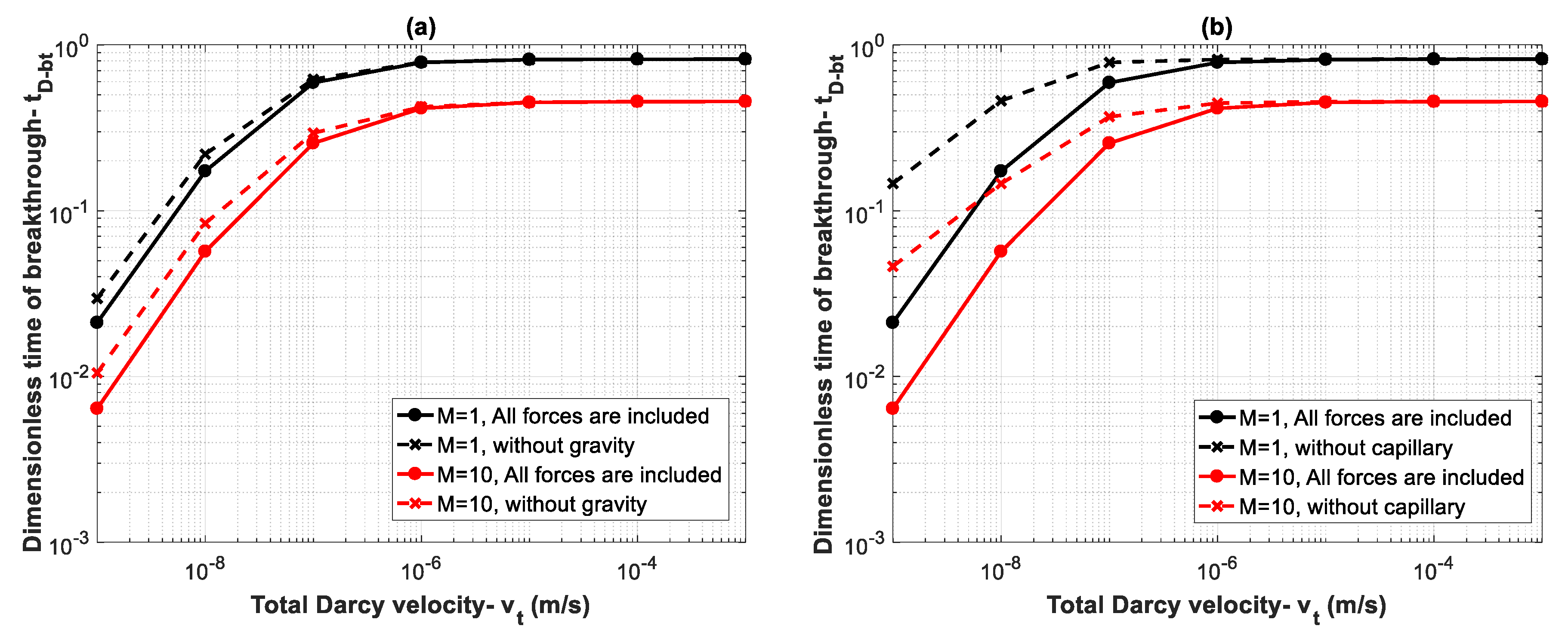Figure 8a shows effects of gravity forces. Continuous lines display the calculated breakthrough time when all forces are included, and the dashed lines show breakthrough time when gravity effects are neglected. The results demonstrate that gravity effects lead to an earlier breakthrough time for small values of ${\mathbf{v}}_t$ due to increasing buoyancy effects. However, as ${\mathbf{v}}_t$ increases (viscous dominated regime), the effect of gravity becomes negligible. Next, we study the effect of capillary forces on breakthrough time. As shown in Figure 8b, capillary forces have a significant effect on breakthrough time for small values of ${\mathbf{v}}_t$. In other words, neglecting capillary effects results in overestimation of breakthrough time. However, the influence of capillary forces becomes negligible by increasing ${\mathbf{v}}_t$.

3.2. Case Study on CO₂ Storage Aquifers in Western Canada

In this section, the developed model is used to study potential CO₂ storage sites in central Alberta, Canada. Province of Alberta has the largest greenhouse gas emissions in Canada, with annual emissions close to 274.1 Mt CO₂ in 2015 [34]. The province is underlain by the Alberta basin, which is suitable for CO₂ geological sequestration in all parts except for its shallow northeastern corner [35]. The largest concentration of CO₂ sources in Alberta is in the Edmonton region where four coal-fired power plants are located near Wabamun Lake, west of Edmonton, which have combined annual CO₂ emissions of more than 30 Mt CO₂ [36]. Figure 9 shows the location of major CO₂ emission sources in central Alberta, Canada. CO₂ sequestration in deep saline aquifers in proximity of these power plants is a promising option for reducing CO₂ atmospheric emissions since the deep coal seams and oil and gas reservoirs in local area do not have sufficient capacity for sequestration of CO₂. Because CO₂ sequestration in geological media and especially in deep saline aquifers is a recently growing field, no relevant measured data have been published regarding displacement characteristics of CO₂–brine systems at in situ conditions until early 2000. Relevant data were only available for CO₂–oil systems for enhanced oil recovery purposes and a handful of measurements for CO₂–oil–brine ternary systems.

To fill the knowledge gap, Bennion and Bachu conducted a series of experiments to measure relative permeability and capillary pressure characteristics at in-situ conditions for CO₂–brine systems [33,37,38,39,40,41,42]. They studied sandstone, carbonate, shale and anhydrite rock formations in the Alberta basin in central Alberta. These formations are general representatives of the in-situ temperature, pressure, and salinity in entire Alberta basin, and likely for all on-shore North American sedimentary basins.

Table 2. In-situ conditions for rock samples from Wabamun Lake area, Alberta basin, Canada [33].

ID *	Unit	Lithology	Depth (m)	Porosity (Fraction)	Pressure (MPa)	Temp. (°C)	Salinity (mg/Liters)
B	Basal Cambrian	Sandstone	2734	0.117	27	75	248,000
E	Ellerslie	Sandstone	1463	0.126	10.9	40	97,217
V	Viking#1	Sandstone	1240	0.125	8.6	35	28,286
C	Cooking lake	Carbonate	1889	0.099	15.4	55	233,417
N	Nisku#1	Carbonate	2050	0.097	17.4	56	136,817
WL	Wabamun #1 (Low Perm)	Carbonate	1353	0.079	11.9	41	144,304
WH	Wabamun #2 (High Perm)	Carbonate	1603	0.148	11.9	41	144,304

* For easy identification in the figures, letters have been assigned to different sample units.

presents a summary of in-situ conditions for the cored intervals from three sandstone and three carbonate formations in the Wabamun Lake area, southwest of Edmonton, Alberta [33,37]. The location of the wells from which core samples were taken is shown in Figure 9. For the Wabamun Group, two samples with low and high permeability were evaluated which results in a total of seven different rock sets. Temperatures in Table 2 are evaluated based on the depth of the samples by considering a geothermal gradient of 25 °C/km [37].

The stratigraphic downhole model for strata in the Wabamun Lake area is available in the literature [37]. Since site specific data for leakage pathways are not available, we used the same data reported for the storage formations to represent the characteristics of the leakage pathway. Nevertheless, the analysis provided is general and allows application of the developed scaling to a leakage pathway when site specific data are available.

Other parameters used in this study are presented in

Table 3. Simulation parameters and calculated values of $M$, $N_{Ca}$ and $N_{Gr}$ for rock samples of Table 2.

Data	Basal Camb.	Ellerslie	Viking	Cooking Lake	Nisku	Wab. Low Perm	Wab. High Perm
Length of domain, $L^{*}$ (m)	500	500	500	500	500	500	500
Brine Viscosity, ${\mu }_w$ (mPa·s)	0.733	0.784	0.755	0.864	0.661	0.863	0.863
CO2 Viscosity, ${\mu }_{nw}$ (mPa·s)	0.062	0.054	0.054	0.056	0.056	0.056	0.056
End-point rel-perm of CO2, $k_{rnw}^{\max }$	0.5446	0.1156	0.3319	0.0685	0.1768	0.5289	0.1883
Absolute permeability, $k$ (mD)	0.081	0.376	2.7	65.3	45.9	0.018	67
Residual Brine Saturation, $S_{wr}$	0.294	0.659	0.558	0.476	0.33	0.595	0.569
Corey Exponent for Brine, $nb$	1.8	2.1	2.9	1.4	2.8	1.4	1.4
Corey Exponent for CO2, $nc$	5	2.2	3.2	5.6	1.1	5.6	2.1
Capillary entry pressure, $p_d^{*}$ (MPa)	0.226	3.382	0.121	0.014	5.794	0.341	0.087
CO2 Density, ${\rho }_{nw}^{*}$ (kg/m3)	723.8	658.1	626.7	645.4	683.3	678.9	678.9
Brine Density, ${\rho }_w^{*}$ (kg/m3)	1140.5	1060.9	1016.9	1138.9	1080.4	1090.5	1090.5
Tilt angle, ${\theta }^{*}$	π/2	π/2	π/2	π/2	π/2	π/2	π/2
Total Buoyancy velocity, ${\mathrm{v}}_t^{*}$ (m/s)	5.34 × 10−9	2.75 × 10−8	1.91 × 10−7	5.65 × 10−6	3.19 × 10−6	1.3 × 10−9	4.83 × 10−6
$M$	6.44	1.68	4.64	1.06	2.09	8.15	2.90
$N_{Ca}$	0.0601	0.1979	0.0210	0.0004	0.5260	0.0893	0.0081
$N_{Gr}$	0.5444	0.1158	0.3322	0.0687	0.1768	0.5290	0.1881

* Estimated values (details are available in the text).

. All the parameters in Table 3, except the ones with asterisk, are taken from measurements of Bennion and Bachu [37,40]. Bennion and Bachu [37] measured relative permeability parameters at reservoir conditions for rock samples of Table 2 and reported absolute permeability, CO₂ and brine viscosity, end-point relative permeability of CO₂ ($k_{rnw}^{\max }$), residual brine saturation ($S_{wr}$), and generated drainage relative permeability curves for CO₂–brine systems. In another paper, Bennion and Bachu [40] reported the fitted Corey exponents based on their measured relative permeability data for rock samples of Table 2. Corey exponents are listed in Table 3. In another work, Bennion and Bachu [38] reported capillary pressure, interfacial tension and pore size distribution characteristics on a series of carbonate and sandstone formations from Wabamun Lake area in Alberta, together with those formations given in Table 2. We used the reported CO₂–brine capillary pressure curves, from their study, and curve-fitted to Equation (15). The evaluated capillary entry pressures ($p_d$) are reported in Table 3.

In Table 3, density of brine is calculated based on Rowe and Chou [43] correlation using temperature, pressure and salt mass fraction for different formations. CO₂ density is calculated using Soave–Redlich–Kwong (SRK) equations of state [44]. Total Darcy velocity (${\mathbf{v}}_t$) in Table 3 is estimated based on ${\mathbf{v}}_t=k\Delta \rho g/{\mu }_{nw}$, which reflects the maximum buoyancy velocity for CO₂ and is calculated using Darcy’s law based on the parameters for each formation. The calculated values in Table 3 are in the range of reported Darcy velocities for CO₂ in the literature [45,46]. In addition, although different velocities could happen in the reservoir, this can be a good measure for comparison of different formations. Finally, we considered a length of 500 m and a tilt angle of $\pi /2$ in this study. Generally, there are no data on the geometry and direction of the leakage pathways for the formations. We considered identical length and tilt angles for the study of all formations to provide a fair comparison between different storage formations.

The calculated values for $M$, $N_{Ca}$ and $N_{Gr}$ are presented in the last three rows of Table 3. The estimated values of mobility ratio have a wide range, starting at 1.06 for Cooking Lake formation to 8.15 for Wabamun Low Perm formation. Estimated values of $N_{Ca}$ and $N_{Gr}$ are shown in a $N_{Gr}-N_{Ca}$ space in Figure 10. A reference equilibrium state between gravitational and viscous forces is indicated with dotted line at $N_{Gr}=1$, and between capillary and viscous forces at $N_{Ca}=1$. As shown in Figure 10, all rock samples fall into the lower left sector where viscous forces dominate over capillary and gravity forces. It is seen that $N_{Ca}$ varies three orders of magnitude, while variations of $N_{Gr}$ are more gradual and fall within one order of magnitude for different formations.

As shown in Figure 10, Cooking Lake carbonate has the lowest capillary and gravity numbers of $N_{Ca}=0.0004$ and $N_{Gr}=0.0687$. The highest effect of gravity forces is in Basal Cambrian sandstone with $N_{Gr}=0.5444$, and the highest effect of capillary forces is in Nisku carbonate with $N_{Ca}=0.5260$.

It is worth mentioning that we used maximum buoyance velocity in the previous calculations. However, velocity of a migrating CO₂ plume may vary within orders of magnitude. To study the effect of total velocity used in our scaling analysis, we perform an analysis to investigate the effect of velocity on the position of various storage formations in the $N_{Gr}-N_{Ca}$ parameter map. Using different values for the total Darcy velocity leads to different capillary and gravity numbers, but the ratio of these forces remains the same. 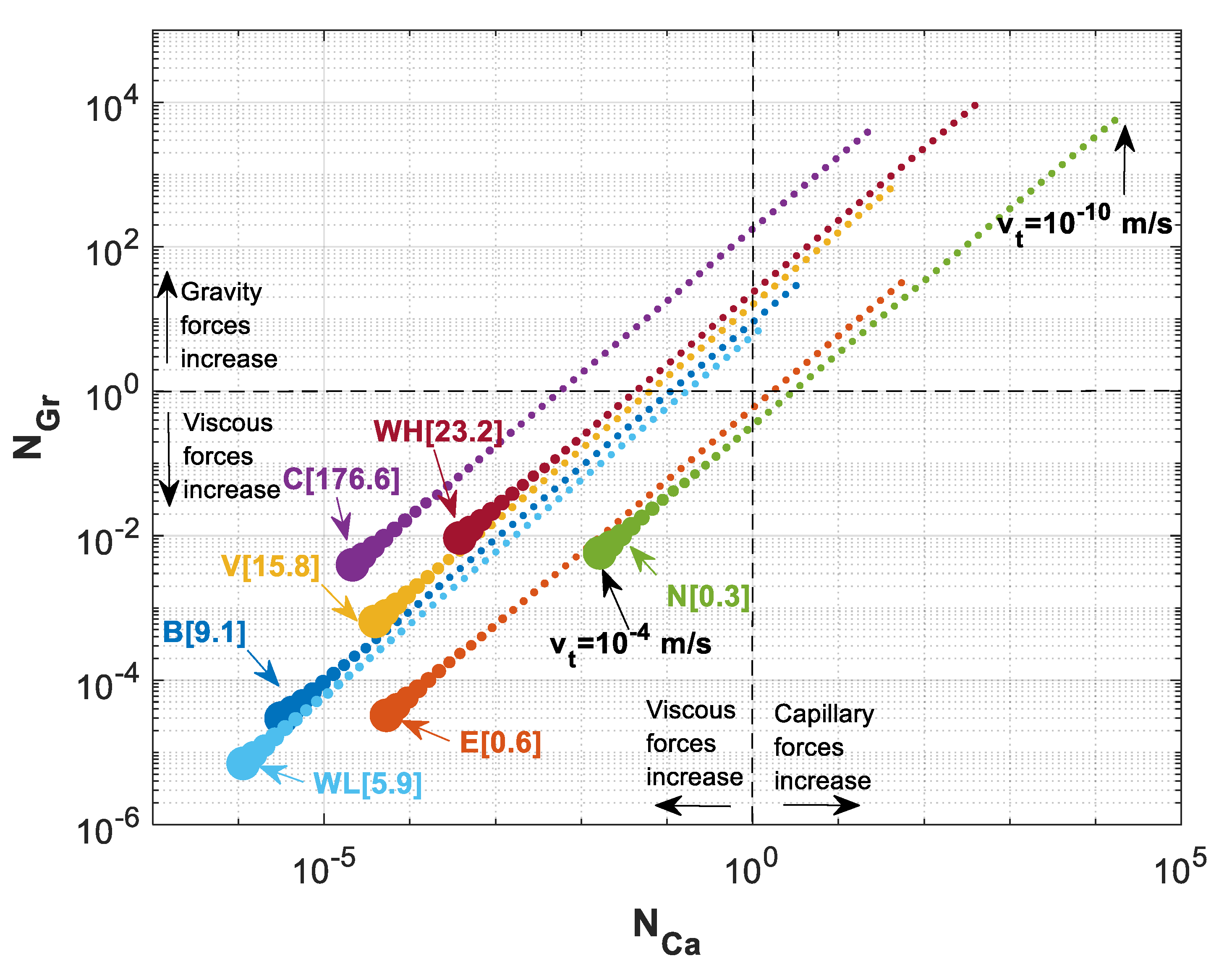Figure 11 shows the estimated values for $N_{Ca}$ and $N_{Gr}$ when total Darcy velocity is varied from 10⁻¹⁰ m/s to 10⁻⁴ m/s for all the formations shown in Table 3. This figure indicates that the ratio of capillary to gravity numbers stays the same as the velocity is changing while various formations have different ratios. In the case of Cooking Lake formation, for instance, while gravity forces are at equilibrium with viscous forces (i.e., $N_{Gr}=1$), capillary forces are greatly dominated by viscous forces ($N_{Ca}=0.006$). On the other hand, for Nisku formation, when $N_{Gr}=1$, capillary number is $N_{Ca}=3.33$, which shows the effects of capillary forces are much higher for Nisku formation than that for Cooking Lake formation.

Other than $N_{Ca}$ and $N_{Gr}$, relative permeability parameters are important in estimations of rate of leakage. Figure 12a–c shows capillary, gravity and viscous functions for all formations shown in Table 3. For all of the rock samples except Nisku and Ellerslie formations, the effect of capillary and gravity forces is reduced due to the small values of $N_{Ca}$ and $N_{Gr}$, and therefore, viscous function, $V(S)$, is the dominant term for estimating saturation and velocity profiles. Mobility ratio as well as Corey exponents of nc and nb determine the behavior of capillary, gravity and viscous functions. As indicated in previous section, a lower mobility ratio and a higher Corey exponent for CO₂ increase the time of breakthrough and the average normalized saturation behind the displacement front. Among the rock samples, Cooking Lake formation has the lowest mobility ratio of $M=1.06$ and highest Corey exponent for CO₂ (nc = 5.6), which results in the highest average saturation behind the displacement front (Figure 12c). In addition, because of small mobility ratio, the values of $D(S)$ and $G(S)$ are relatively high for this case, though their effect on velocity profile is insignificant. Despite similar Corey exponents (nc and nb) of Wabamun Low Perm and Cooking Lake formation, mobility ratio is higher and equal to $M=8.15$ for Wabamun Low Perm. Further, by comparing these formations (Figure 12a,b), it can be inferred that Wabamun Low Perm has smaller $D(S)$ and $G(S)$ values in comparison to Cooking Lake formation, and the average saturation behind the displacement front is lower for Wabamun Low Perm as well (see Figure 12c). For Basal Cambrian sandstone, mobility ratio is relatively high ($M=6.44$), however, the average saturation behind the displacement front is also high, since Corey exponent for CO₂ is nc = 5 (Figure 12c). Therefore, contribution of $D(S)$ and $G(S)$ are negligible due to the value of mobility ratio (Figure 12a,b). Nisku formation has the lowest Corey exponent for CO₂, nc = 1.1, and even though the mobility ratio for this formation is relatively small and equal to M = 2.09, it has the lowest average saturation behind the displacement front (Figure 12c). Additionally, as shown in Figure 12a,b, contribution of $D(S)$ and $G(S)$ are relatively high for this dataset. Finally, the behavior of capillary, gravity and viscous functions for Wabamun High Perm and Ellerslie formations are very similar, since their mobility ratios and Corey exponents are almost equal.

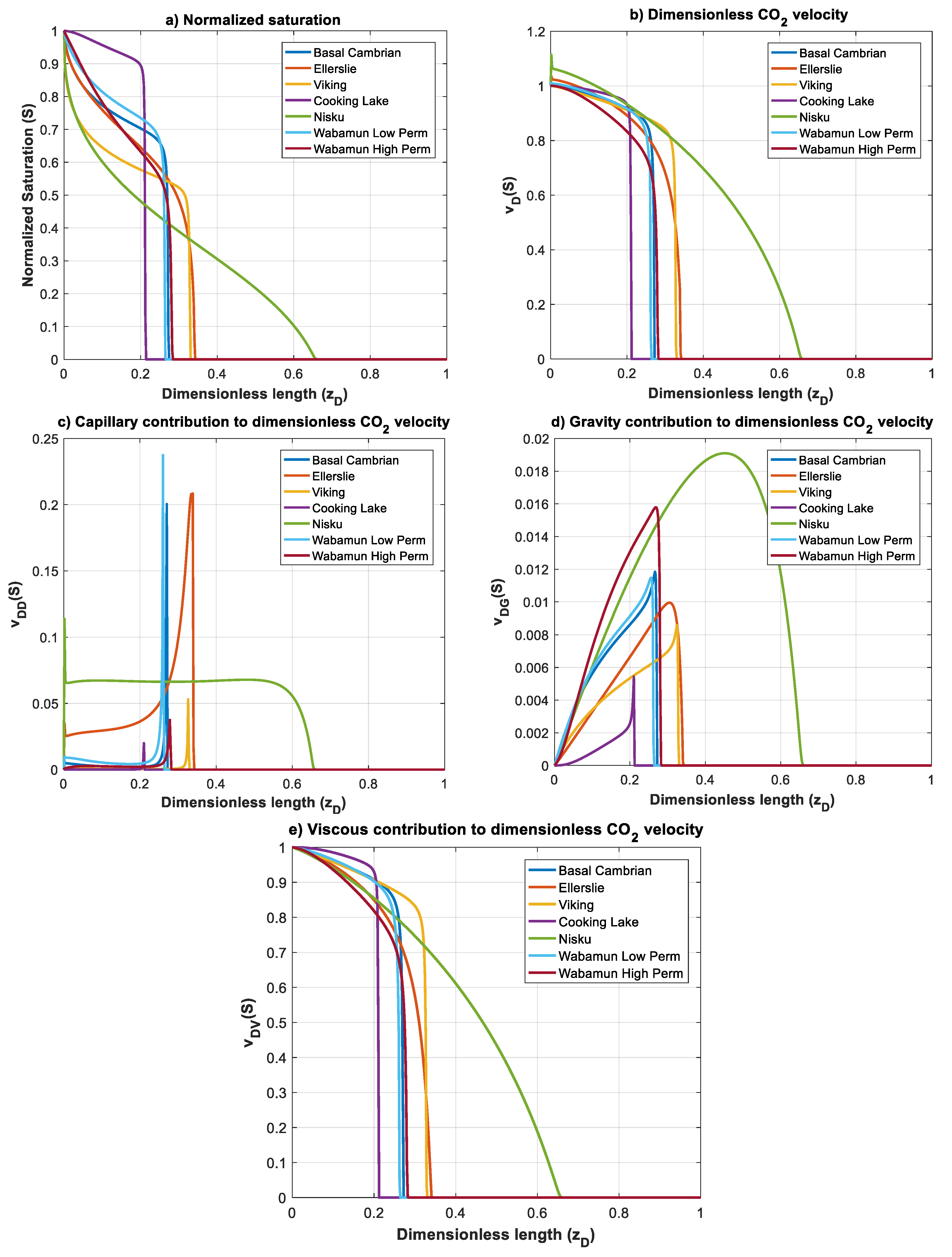
Figure 13 shows the normalized gas saturation and contribution of different forces on CO₂ dimensionless velocity, for all rock samples at time $t_D=0.2$. It can be immediately observed that, due to the domination of viscous forces over capillary and gravity forces (small values of $N_{Ca}$ and $N_{Gr}$), plume evolution and the dimensionless velocity greatly resemble the viscous function $V(S)$, for all formations, except Nisku and Ellerslie, for which capillary forces are relatively high. Nisku formation has the fastest plume evolution and a countercurrent flow of brine is observed at the inlet due to the effect of capillary forces (Figure 13b,c). Same as Nisku formation, Ellerslie formation does not develop a sharp font, and contribution of capillary forces on velocity causes a small countercurrent flow of brine at the inlet.

CO₂ front is relatively sharp for the rest of the formations. The front propagation for Cooking Lake formation is slow compared to other formations, which is due to the small mobility ratio and high nc, as well as small $N_{Ca}$ and $N_{Gr}$. Shapes of the CO₂ plume and velocity profiles are similar for Basal Cambrian and Wabamun Low Perm formations. This is because of their position on $N_{Gr}-N_{Ca}$ map (Figure 10) and similar values of mobility ratio and nc (Table 3). Again, in the above analysis, we used maximum buoyance velocity. However, velocity of a migrating CO₂ plume may vary within orders of magnitude, which can change the position of the formations in the $N_{Gr}-N_{Ca}$ parameter map. Nevertheless, the scaling analysis provided is general and allows application to specific storage site when site specific data are available.

The average normalized gas saturation versus dimensionless time for all the formations are shown in Figure 14, which are in good agreement with the saturation and velocity profiles discussed earlier. For instance, for the Cooking Lake formation, the breakthrough of CO₂ is delayed due to the less diffusive nature of the displacement front, whereas in the Nisku formation, the effect of capillary forces leads to a diffusive shape front and therefore an earlier breakthrough is expected with lower CO₂ saturation.

Since the discussed values are dimensionless, further discussion on the real time of breakthrough and the cumulative amount of leaked CO₂ requires site specific data such as residual brine saturation and porosity of the formations. These parameters are not identical for all the formations and taking these parameters into account would influence the interpretation of results, as described in the following.

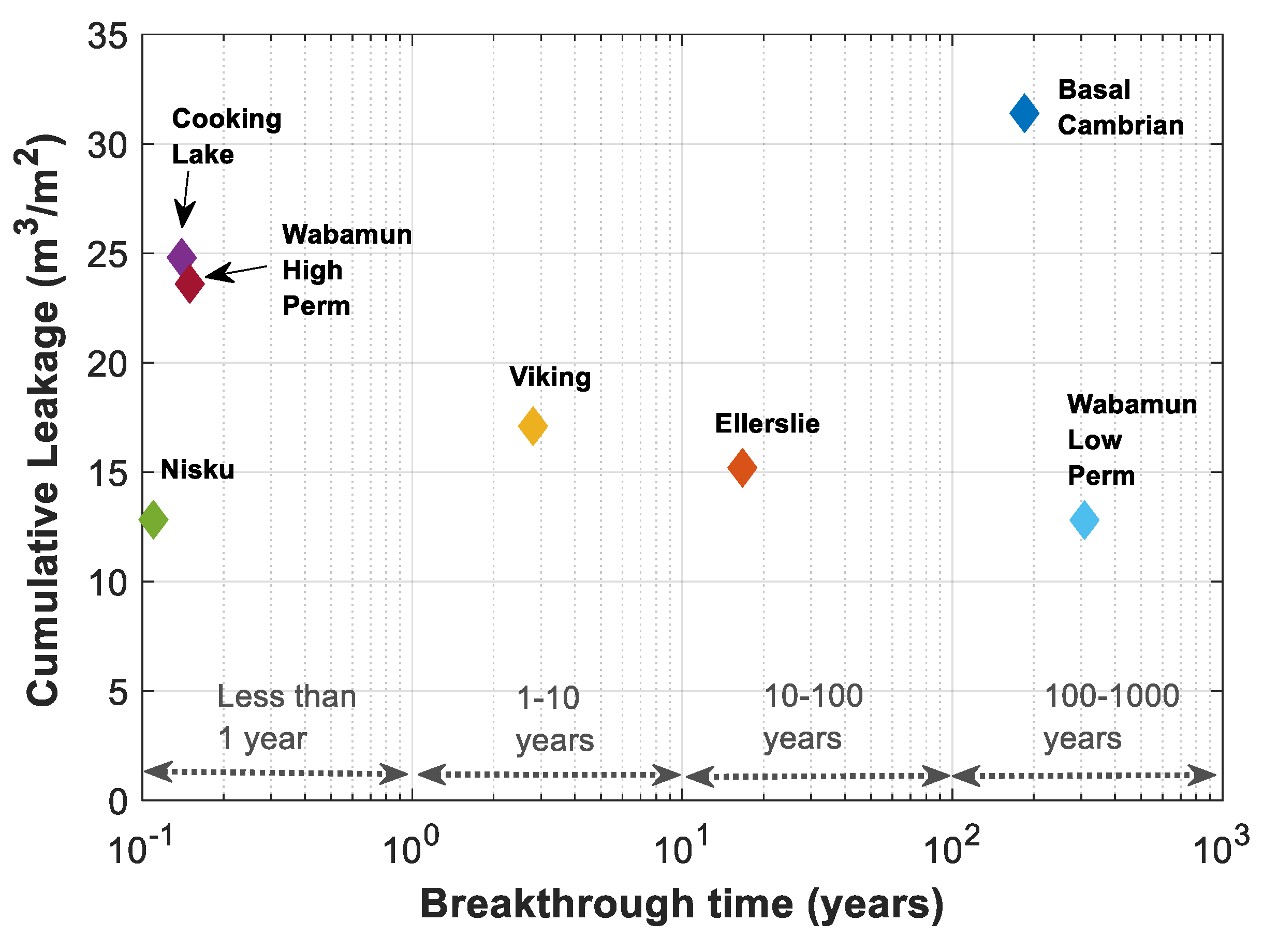
The real time of breakthrough and cumulative amount of leakage are calculated based on the dimensionless time of breakthrough and the average normalized saturation in Figure 14 and

Table 4. Time of breakthrough and cumulative leakage calculated for different formations of Table 3.

Formation	Dimensionless Time of Breakthrough, ${\mathit{t}}_{\mathit{D}-\mathit{b}\mathit{t}}$	Total Buoyancy Velocity, ${\mathit{v}}_{\mathit{t}}$ (m/s)	Real time of Breakthrough, $\mathit{t}$ (Years)	Average Normalized Saturation, $\overline{\mathit{S}}$	Cumulative Leakage at Time of Breakthrough, (m3/m2)
Basal Cambrian	0.7544	5.34 × 10−9	185.0	0.7611	31.4
Ellerslie	0.6747	2.75 × 10−8	16.7	0.7070	15.2
Viking	0.6161	1.91 × 10−7	2.8	0.6184	17.1
Cooking Lake	0.9532	5.65 × 10−6	0.14	0.9542	24.8
Nisku	0.3396	3.19 × 10−6	0.11	0.3949	12.83
Wab. Low Perm	0.7893	1.3 × 10−9	308.5	0.8007	12.81
Wab. High Perm	0.7355	4.83 × 10−6	0.15	0.7390	23.6

. The dimensionless time of breakthrough is converted to the real time of breakthrough using Equations (9) and (10), and the cumulative amount of leakage per m² of the cross-sectional area of the migration pathway is calculated using $\overline{S}\times (1-S_{wr})\times L\times \varphi$, where $S_{wr}$ is the brine residual saturation and $\overline{S}$ is the average normalized saturation, $\overline{S}={\displaystyle \underset{0}{\overset{1}{\int }}Sd{z}_D}$. The cumulative amount of leakage is plotted versus time for all formations in Figure 15. As expected, the results are different from what has been expected based on Figure 14. This is essentially due to the different values of residual brine saturation and porosity of different formations.

The maximum Darcy buoyancy velocity considered for each formation has a great impact on estimating the breakthrough time. Cooking Lake, Wabamun High Perm, and Nisku formations have the highest Darcy buoyancy velocities and thus lower estimated breakthrough times of 51, 56, and 40 days, respectively. Darcy buoyancy velocity decreases for Viking, Ellerslie, Basal Cambrian and Wabamun Low Perm formations, respectively, and as can be seen in Figure 15, time of breakthrough is delayed for these formations, correspondingly. Porosity times maximum saturation, ${\varphi }^{*}=(1-S_{wr})\times \varphi$, gives an estimate of the available pore volume for CO₂.

In addition, time of breakthrough is highest for Wabamun Low Perm formation, (~308 years), since the estimated Darcy velocity is lowest for this case compared to the other formations, (${\mathbf{v}}_t=1.3\times {10}^{-9}$), and at the same time, the amount of leaked CO₂ is lowest for this case, due to the small pore volume available for fluids flow (${\varphi }^{*}=0.03$). A possible leakage from a storage aquifer through a leakage pathway can be remediated specially if detected early enough. On the other hand, chances of contribution of other trapping mechanisms and therefore reducing the amount of leakage is higher for cases with higher time of leakage, such as Wabamun Low Perm or Basal Cambrian formations.

Celia et al. [47] assessed risk of brine and CO₂ leakage through abandoned wells in the same area that we discussed here (as depicted in Figure 9). They simulated 50 years of CO₂ injection using a semi-analytical modeling approach over a study area of 2500 km². They concluded that the behavior of the system is dependent on the interplay of formation and fluid properties, maximum injectivity of the formation and the properties of the leaky wells. Generally, lower number of oil and gas wells penetrate the caprocks of deeper formations and this will clearly result in a tradeoff between depth of injection and risk of leakage. However, their simulations imply that the number and design of the injection wells and injectivity of the formations play a critical role on the assessment of leakage. Due to lack of data, they assigned the well permeabilities based on the probability distribution. With their assumption of a single vertical injection well and considering the limitation of injectivity, they concluded that Nisku and the Basal Cambrian formations are the two viable options for CO₂ injection.

4. Conclusions

In this study, a numerical model is developed to investigate the influence of driving forces on CO₂ plume evolution and breakthrough time during a leakage from a water saturated pathway. The results of this study can be used for estimation of leakage for different potential CO₂ storage sites where formation properties of leakage pathways are available.

Dimensionless terms of $D(S)$, $G(S)$ and $V(S)$ along with dimensionless capillary and gravity numbers are introduced to express the effect and ratio of capillary, gravity and viscous forces. A leakage process is characterized by a two-phase system, in which the non-wetting and less viscous CO₂ displaces the resident brine. Results from this study show that increasing the effect of gravity forces (and therefore $N_{Gr}$) leads to an earlier breakthrough of CO₂. Similar to $N_{Gr}$, by increasing the effect of capillary forces ($N_{Ca}$) a diffusive-like front is established, which also results in an earlier breakthrough. At high values of $N_{Ca}$, a backward flow of brine is observed as CO₂ migrates upward. For high $N_{Ca}$, the saturation distribution is diffusive in nature, which results in a gradually leaking CO₂. In terms of operations, a sharp front leakage may be more problematic than a gradual leakage (diffusive dominated flow) since it is more difficult to take remedial actions to prevent leakage in case of a sudden release of CO₂. Additionally, it is seen that the effect of increasing $N_{Gr}$ by one order of magnitude on accelerating the breakthrough time, is much less than that of increasing $N_{Ca}$.

The relative permeability–saturation relationships have shown to be of great influence for plume evolution. Results show that a low relative permeability of CO₂ (low end-point relative permeability of CO₂ or high Corey exponent for CO₂) results in a more compact plume evolution. A compact front propagation results in a delayed breakthrough but has the risk of a sudden release of a large volume of leaked CO₂.

The developed numerical model was applied to different potential storage formations in Western Canada. In the absence of site specific data for leakage pathways, data reported for the corresponding storage formations were used. Nevertheless, the presented analysis provided is general and allows application of the developed scaling to specific leakage pathway when data are available. For these formations, it is seen that $N_{Ca}$ varies within three orders of magnitude, while variations of $N_{Gr}$ are more gradual and fall within one order of magnitude. In addition, due to small values of $N_{Ca}$ and $N_{Gr}$, plume evolution and the dimensionless velocity greatly resemble the viscous function, $V(S)$, for all formations, except Nisku and Ellerslie, for which capillary forces are relatively high. It is worth mentioning that, for scaling analysis, we used the maximum buoyancy velocity for different formations, however the velocity of a migrating CO₂ plume may vary within orders of magnitude which may change the position of various storage formations in the $N_{Gr}-N_{Ca}$ parameter map. Comparing different formations in Alberta basin revealed that in determining time of breakthrough and the cumulative amount of leaked CO₂, parameters such as residual brine saturation and porosity of the medium are critical and significantly contribute to the interpretation of results.

The numerical models presented in this paper predict displacement process for a one-dimensional homogenous media. However, the processes induced by CO₂ leakage may be quite complex and may operate on a broad range of space and timescales. For instance, viscous fingering may significantly alter the shape of CO₂–water displacement front, creates channels with high CO₂ effective permeability and thus earlier leakage of CO₂. In addition, the leaked CO₂ may undergo phase changes due to temperature variations, which have not been considered in this study. Therefore, further research should consider temperature variation as well as two- and three-dimensional models with detailed representation of leakage pathways heterogeneities for a more realistic representation of the problem.

References

1. IPCC (Intergovernmental Panel on Climate Change). Special Report on Carbon Dioxide Capture and Storage; Metz, B., Davidson, O., De Coninck, H., Loos, M., Meyer, L., Eds.; Prepared by Working Group III of the Intergovernmental Panel on Climate Change; Cambridge University Press: Cambridge, UK; New York, NY, USA, 2005. [Google Scholar]
2. Le Quéré, C.; Moriarty, R.; Andrew, R.M.; Peters, G.P.; Ciais, P.; Friedlingstein, P.; Jones, S.D. Global carbon budget 2014. Earth Syst. Sci. Data 2015, 7, 47–85. [Google Scholar] [CrossRef] [Green Version]
3. Makhnenko, R.Y.; Vilarrasa, V.; Mylnikov, D.; Laloui, L. Hydromechanical aspects of CO2 breakthrough into clay-rich caprock. In Energy Procedia; Elsevier: Amsterdam, The Netherlands, 2017; Volume 114, pp. 3219–3228. [Google Scholar]
4. Emami-Meybodi, H.; Hassanzadeh, H.; Green, C.P.; Ennis-King, J. Convective dissolution of CO2 in saline aquifers: Progress in modeling and experiments. Int. J. Greenh. Gas Control 2015, 40, 238–266. [Google Scholar] [CrossRef]
5. Bear, J. Dynamics of Fluids in Porous Media; Elsevier: New York, NY, USA, 1972. [Google Scholar]
6. Nordbotten, J.M.; Celia, M.A.; Bachu, S. Injection and storage of CO2 in deep saline aquifers: Analytical solution for CO2 plume evolution during injection. Transp. Porous Media 2005, 58, 339–360. [Google Scholar] [CrossRef]
7. Dentz, M.; Tartakovsky, D.M. Abrupt-interface solution for carbon dioxide injection into porous media. Transp. Porous Media 2009, 79, 15–27. [Google Scholar] [CrossRef]
8. Vilarrasa, V.; Bolster, D.; Dentz, M.; Olivella, S.; Carrera, J. Effects of CO2 compressibility on CO2 storage in deep saline aquifers. Transp. Porous Media 2010, 85, 619–639. [Google Scholar] [CrossRef] [Green Version]
9. Houseworth, J.E. Matched boundary extrapolation solutions for CO2 well-injection into a saline aquifer. Transp. Porous Media 2012, 91, 813–831. [Google Scholar] [CrossRef]
10. Ide, S.T.; Jessen, K.; Orr, F.M. Storage of CO2 in saline aquifers: Effects of gravity, viscous, and capillary forces on amount and timing of trapping. Int. J. Greenh. Gas Control 2007, 1, 481–491. [Google Scholar] [CrossRef]
11. Kopp, A.; Class, H.; Helmig, R. Investigations on CO2 storage capacity in saline aquifers. Part 1. Dimensional analysis of flow processes and reservoir characteristics. Int. J. Greenh. Gas Control 2009, 3, 263–276. [Google Scholar] [CrossRef]
12. Kopp, A.; Class, H.; Helmig, R. Investigations on CO2 storage capacity in saline aquifers-Part 2: Estimation of storage capacity coefficients. Int. J. Greenh. Gas Control 2009, 3, 277–287. [Google Scholar] [CrossRef]
13. Bachu, S.; Celia, M.A. Assessing the potential for CO2 leakage, particularly through wells, from geological storage sites. Geophys. Monogr. Ser. 2009, 183, 203–216. [Google Scholar] [CrossRef]
14. Laurich, B.; Urai, J.L.; Desbois, G.; Vollmer, C.; Nussbaum, C. Microstructural evolution of an incipient fault zone in Opalinus Clay: Insights from an optical and electron microscopic study of ion-beam polished samples from the Main Fault in the Mt-Terri Underground Research Laboratory. J. Struct. Geol. 2014, 67, 107–128. [Google Scholar] [CrossRef]
15. Zoback, M.D.; Gorelick, S.M. Earthquake triggering and large-scale geologic storage of carbon dioxide. Proc. Natl. Acad. Sci. USA 2012, 109, 10164–10168. [Google Scholar] [CrossRef] [PubMed] [Green Version]
16. Vilarrasa, V.; Carrera, J. Geologic carbon storage is unlikely to trigger large earthquakes and reactivate faults through which CO2 could leak. Proc. Natl. Acad. Sci. USA 2015, 112, 5938–5943. [Google Scholar] [CrossRef] [PubMed]
17. Haekes, C.D.; McLellan, P.J.; Bachu, S. Geomechanical factors affecting geological storage of CO2 in depleted oil and gas reservoirs. J. Can. Pet. Technol. 2005, 44, 52–61. [Google Scholar] [CrossRef]
18. Rutqvist, J. The Geomechanics of CO2 storage in deep sedimentary formations. Geotech. Geol. Eng. 2012, 30, 525–551. [Google Scholar] [CrossRef]
19. Celia, M.A.; Nordbotten, J.M.; Bachu, S.; Dobossy, M.; Court, B. Risk of leakage versus depth of injection in geological storage. Energy Procedia 2009, 1, 2573–2580. [Google Scholar] [CrossRef]
20. Nordbotten, J.M.; Celia, M.A.; Bachu, S.; Dahle, H.K. Semianalytical solution for CO2 leakage through an abandoned well. Environ. Sci. Technol. 2005, 39, 602–611. [Google Scholar] [CrossRef] [PubMed]
21. Nordbotten, J.M.; Celia, M.A.; Bachu, S. Analytical solutions for leakage rates through abandoned wells. Water Resour. Res. 2004, 40. [Google Scholar] [CrossRef] [Green Version]
22. Nordbotten, J.M.; Kavetski, D.; Celia, M.A.; Bachu, S. Model for CO2 leakage including multiple geological layers and multiple leaky wells. Environ. Sci. Technol. 2009, 43, 743–749. [Google Scholar] [CrossRef] [PubMed]
23. Dejam, M.; Hassanzadeh, H. Diffusive leakage of brine from aquifers during CO2 geological storage. Adv. Water Resour. 2018, 111, 36–57. [Google Scholar] [CrossRef]
24. Dejam, M.; Hassanzadeh, H. The role of natural fractures of finite double-porosity aquifers on diffusive leakage of brine during geological storage of CO2. Int. J. Greenh. Gas Control 2018, 78, 177–197. [Google Scholar] [CrossRef]
25. Pruess, K. Leakage of CO2 from geologic storage: Role of secondary accumulation at shallow depth. Int. J. Greenh. Gas Control 2008, 2, 37–46. [Google Scholar] [CrossRef]
26. Rinaldi, A.P.; Jeanne, P.; Rutqvist, J.; Cappa, F.; Guglielmi, Y. Effects of fault-zone architecture on earthquake magnitude and gas leakage related to CO2 injection in a multi-layered sedimentary system. Greenh. Gases Sci. Technol. 2014, 4, 99–120. [Google Scholar] [CrossRef]
27. Rinaldi, A.P.; Vilarrasa, V.; Rutqvist, J.; Cappa, F. Fault reactivation during CO2 sequestration: Effects of well orientation on seismicity and leakage. Greenh. Gases Sci. Technol. 2015, 5, 645–656. [Google Scholar] [CrossRef]
28. Rutqvist, J.; Rinaldi, A.P.; Cappa, F.; Jeanne, P.; Mazzoldi, A.; Urpi, L.; Guglielmi, Y.; Vilarrasa, V. Fault activation and induced seismicity in geologic carbon storage—Lessons learned from recent modeling studies. J. Rock Mech. Geotech. Eng. 2016, 8, 789–804. [Google Scholar] [CrossRef]
29. Kang, M.; Nordbotten, J.M.; Doster, F.; Celia, M.A. Analytical solutions for two-phase subsurface flow to a leaky fault considering vertical flow effects and fault properties. Water Resour. Res. 2014, 50, 3536–3552. [Google Scholar] [CrossRef] [Green Version]
30. Brooks, R.; Corey, A. Hydraulic Properties of Porous Media; Hydro Paper; Colorado State University: Fort Collins, CO, USA, 1964. [Google Scholar]
31. Firoozabadi, A.; Ishimoto, K. Reinfiltration in fractured porous media: Part 1—One dimensional model. SPE Adv. Technol. Ser. 1994, 2, 35–42. [Google Scholar] [CrossRef]
32. Rosado-Vazquez, F.J.; Rangel-German, E.R.; Rodriguez-De La Garza, F. Analytical model for vertical oil/water displacement under combined viscous, capillary, and gravity effects. In SPE Western Regional/AAPG Pacific Section/GSA Cordilleran Section Joint Meeting; Society of Petroleum Engineers: Anchorage, AK, USA, 2006. [Google Scholar]
33. Bachu, S.; Bennion, B. Effects of in-situ conditions on relative permeability characteristics of CO2-brine systems. Environ. Geol. 2008, 54, 1707–1722. [Google Scholar] [CrossRef]
34. Environment and Climate Change Canada. Canadian Environmental Sustainability Indicators: Greenhouse Gas Emissions. 2017. Available online: http://www.ec.gc.ca/indicateurs-indicators/18F3BB9C-43A1-491E-9835-76C8DB9DDFA3/GHGEmissions_EN.pdf (accessed on 1 April 2017).
35. Bachu, S. Screening and ranking of sedimentary basins for sequestration of CO2 in geological media in response to climate change. Environ. Geol. 2003, 44, 277–289. [Google Scholar] [CrossRef]
36. Michael, K.; Bachu, S.; Buschkuehle, B.E.; Haug, K.; Talman, S. Comprehensive characterization of a potential site for CO2 geological storage in central Alberta, Canada. In Carbon Dioxide Sequestration in Geological Media—State of the Science: AAPG Studies in Geology; The American Association of Petroleum Geologists: Tulsa, OK, USA, 2009; pp. 227–240. [Google Scholar] [CrossRef]
37. Bennion, B.; Bachu, S. Relative permeability characteristics for supercritical CO2 displacing water in a variety of potential sequestration zones in the Western Canada sedimentary basin. In SPE Annual Technical Conference and Exhibition; Society of Petroleum Engineers: Dallas, TX, USA, 2005. [Google Scholar]
38. Bennion, B.; Bachu, S. The impact of interfacial tension and pore-size distribution/capillary pressure character on CO2 relative permeability at reservoir conditions in CO2-brine systems. In SPE/DOE Symposium on Improved Oil Recovery; Society of Petroleum Engineers: Tulsa, OK, USA, 2006. [Google Scholar]
39. Bennion, D.B.; Bachu, S. Dependence on temperature, pressure, and salinity of the IFT and relative permeability displacement characteristics of CO2 injected in deep saline aquifers. In SPE Annual Technical Conference and Exhibition; Society of Petroleum Engineers: San Antonio, TX, USA, 2006. [Google Scholar]
40. Bennion, B.; Bachu, S. Drainage and imbibition relative permeability relationships for supercritical CO2/Brine and H2S/Brine systems in intergranular sandstone, carbonate, shale, and anhydrite rocks. SPE Reserv. Eval. Eng. 2008, 11, 487–496. [Google Scholar] [CrossRef]
41. Bennion, D.B.; Bachu, S. Drainage and imbibition CO2/brine relative permeability curves at reservoir conditions for carbonate formations. In SPE Annual Technical Conference and Exhibition; Society of Petroleum Engineers: Florence, Italy, 2010. [Google Scholar]
42. Bachu, S. Drainage and imbibition CO2/brine relative permeability curves at in situ conditions for sandstone formations in Western Canada. Energy Procedia 2013, 37, 4428–4436. [Google Scholar] [CrossRef]
43. Rowe, A.M.; Chou, J.C.S. Pressure-volume-temperature-concentration relation of aqueous sodium chloride solutions. J. Chem. Eng. Data 1970, 15, 61–66. [Google Scholar] [CrossRef]
44. Hassanzadeh, H.; Pooladi-Darvish, M.; Elsharkawy, A.M.; Keith, D.W.; Leonenko, Y. Predicting PVT data for CO2-brine mixtures for black-oil simulation of CO2 geological storage. Int. J. Greenh. Gas Control 2008, 2, 65–77. [Google Scholar] [CrossRef]
45. Berg, S.; Ott, H. Stability of CO2-brine immiscible displacement. Int. J. Greenh. Gas Control 2012, 11, 188–203. [Google Scholar] [CrossRef]
46. Polak, S.; Cinar, Y.; Holt, T.; Torsæter, O. Use of low- and high-IFT fluid systems in experimental and numerical modelling of systems that mimic CO2 storage in deep saline formations. J. Pet. Sci. Eng. 2015, 129, 97–109. [Google Scholar] [CrossRef] [Green Version]
47. Celia, M.A.; Nordbotten, J.M.; Court, B.; Dobossy, M.; Bachu, S. Field-scale application of a semi-analytical model for estimation of CO2 and brine leakage along old wells. Int. J. Greenh. Gas Control 2011, 5, 257–269. [Google Scholar] [CrossRef]
48. Hassanzadeh, H.M.; Pooladi-Darvish, M.; Keith, D.W. Modelling of convective mixing in CO2 storage. J. Can. Pet. Technol. 2005, 44, 43–51. [Google Scholar] [CrossRef]
49. Ozisik, M.N. Heat Conduction; John Wiley & Sons: New York, NY, USA, 1993; ISBN 0471532568. [Google Scholar]
50. Buckley, S.E.; Leverett, M.C. Mechanism of Fluid Displacement in Sands. Trans. AIME 1942, 146, 107–116. [Google Scholar] [CrossRef]
Figure 1. Pathways for CO2 migration for a possible leakage through faults (Adapted from Bachu and Celia [13]).
Fluids 03 00080 g001
Figure 2. Schematic of the problem.
Fluids 03 00080 g002
Figure 3. Gravity number, N G r , versus capillary number, N C a , for Datasets 1–7 defined in Table 1.
Fluids 03 00080 g003
Figure 4. (a) Capillary function, D ( S ) ; (b) gravity function, G ( S ) ; and (c) viscous function, V ( S ) , for Datasets 1 to 7 from Table 1.
Fluids 03 00080 g004
Figure 5. Normalized CO2 saturation and dimensionless CO2 velocity profiles versus dimensionless length at t D = 0.2 for Datasets 1–4 (Table 1): (a) normalized saturation; (b) dimensionless CO2 velocity, v D ; (c) capillary contribution to CO2 velocity, v D D ; (d) gravity contribution to CO2 velocity, v D G ; and (e) viscous contribution to CO2 velocity, v D V .
Fluids 03 00080 g005
Figure 6. Average saturation versus dimensionless time ( t D ) for: (a) Datasets 1–4 (Table 1) to show the effect of varying N C a and N G r ; and (b) Datasets 1 and 5–7 (Table 1) to show the effect of relative permeability parameters M , nc and nb.
Fluids 03 00080 g006
Figure 7. Normalized CO2 saturation and dimensionless CO2 velocity profiles versus dimensionless length at t D = 0.2 for Datasets 1 and 5–7 (Table 1): (a) normalized saturation; (b) dimensionless CO2 velocity, v D ; (c) capillary contribution to CO2 velocity, v D D ; (d) gravity contribution to CO2 velocity, v D G ; and (e) viscous contribution to CO2 velocity, v D V .
Fluids 03 00080 g007aFluids 03 00080 g007b
Figure 8. Influence of (a) gravity forces and (b) capillary forces on breakthrough time with varying velocity from 1 × 10⁻⁹ m/s to 1 × 10⁻³ m/s for two mobility ratios of M = 1 (Dataset 5) and M = 10 (Dataset 1).
Fluids 03 00080 g008
Figure 9. Location of large stationary CO2 sources in central Alberta, Canada and wells with core samples used in experiments [33].
Fluids 03 00080 g009
Figure 10. Gravity number ( N G r ) versus capillary number ( N C a ) for different formations in Table 3.
Fluids 03 00080 g010
Figure 11. N G r versus N C a for a varying total Darcy velocity ( v t ) ranging from 10−10 m/s to 10−4 m/s for different formations of Table 3. The numbers in brackets is the ratio of N G r / N C a for different formations.
Fluids 03 00080 g011
Figure 12. (a) Capillary function D ( S ) ; (b) gravity function G ( S ) ; and (c) viscous function, V ( S ) , for different rock samples of Table 2.
Fluids 03 00080 g012
Figure 13. Normalized CO2 saturation and dimensionless CO2 velocity profiles versus dimensionless length at t D = 0.2 for rock samples in Table 3: (a) normalized saturation; (b) dimensionless CO2 velocity, v D ; (c) capillary contribution to CO2 velocity, v D D ; (d) gravity contribution to CO2 velocity, v D G ; and (e) viscous contribution to CO2 velocity, v D V .
Fluids 03 00080 g013
Figure 14. Average normalized saturation versus dimensionless time ( t D ) for rock samples in Table 2.
Fluids 03 00080 g014
Figure 15. Cumulative leakage per m2 of leakage pathway versus time for rock samples of Table 3.
Fluids 03 00080 g015