Quasi-Steady versus Navier–Stokes Solutions of Flapping Wing Aerodynamics

Abstract

Various tools have been developed to model the aerodynamics of flapping wings. In particular, quasi-steady models, which are considerably faster and easier to solve than the Navier–Stokes equations, are often utilized in the study of flight dynamics of flapping wing flyers. However, the accuracy of the quasi-steady models has not been properly documented. The objective of this study is to assess the accuracy of a quasi-steady model by comparing the resulting aerodynamic forces against three-dimensional (3D) Navier–Stokes solutions. The same wing motion is prescribed at a fruit fly scale. The pitching amplitude, axis, and duration are varied. Comparison of the aerodynamic force coefficients suggests that the quasi-steady model shows significant discrepancies under extreme pitching motions, i.e., the pitching motion is large, quick, and occurs about the leading or trailing edge. The differences are as large as 1.7 in the cycle-averaged lift coefficient. The quasi-steady model performs well when the kinematics are mild, i.e., the pitching motion is small, long, and occurs near the mid-chord with a small difference in the lift coefficient of 0.01. Our analysis suggests that the main source for the error is the inaccuracy of the rotational lift term and the inability to model the wing-wake interaction in the quasi-steady model.

1. Introduction

A preliminary version of this paper was presented at the AIAA SciTech Conference, Grapevine, Texas, in 2017 [1].

Micro air vehicles (MAVs), typically 15 cm or less in size, will likely be used in a host of applications in the coming years, from military use cases to agricultural and industrial functions, and even recreational pursuits. The small size of MAVs can result in many beneficial qualities such as high maneuverability, low operating costs, as well as being inconspicuous. However, MAVs come with their own set of technical challenges, which is why they are currently still an area of active research. It was only recently through the miniaturization of electronics as well as the ability to fabricate micro-scale parts from a variety of materials that MAVs can start to be realized [2]. In addition to the challenges associated with manufacture of MAVs, the design of MAVs is also hampered by the complex aerodynamics of flapping wing flight, which are quite different from the aerodynamics that govern larger manned vehicles. In particular, they operate under a Reynolds number that is orders of magnitude smaller, i.e., O(10²)–O(10⁴), as opposed to O(10⁶) or higher for more conventional aircraft. Operating in this regime introduces new challenges associated with aerodynamic efficiency and lift generation, while their small size makes them particularly susceptible to environmental factors leading to challenges associated with stability and control [3,4,5].

While still not available in the market, a number of prototype flapping wing MAVs have been created by research groups. A majority of these small robotic fliers have wing and body shapes that are similar to those found in nature. Biological fliers have many desirable traits that would be beneficial for MAVs. For flapping wing MAVs, there has been a considerable amount of research into insects such as flies, bees, hawkmoths, etc. both computationally and experimentally [4,6,7,8,9,10,11,12,13,14,15,16]. Experimental research allows researchers to observe how biological fliers work, to inform the design of biomimetic and biological inspired MAVs, and to compare against the performance of current MAV designs. However, experimental research can be challenging, especially at these small scales. In addition, experimental research does not allow for MAV designs to be tested and assessed before being produced. Computational techniques allow for different design configurations, kinematics, as well as different models to be tested before creating a prototype. There are a variety of computational techniques, ranging from accurate (but time consuming) Navier–Stokes equation (NSe) solution methods to simplified (yet fast) quasi-steady (QS) models.

QS models have long been used since they allow for simple algebraic equations to express the aerodynamic forces. This computational efficiency allows for the model to be used for quickly checking the effects of changing key design parameters, such as flapping and pitching amplitude, pitching duration, pitching axis, and wing geometries. This is particularly important for MAVs because their small size and operating speeds, lift and thrust need to be produced with moving wings. Weis-Fogh [6] was one of the first to pioneer the QS model for flapping wings, describing a method called the steady state principle. The QS model ignores the effects of flow history and instead considers the forces generated only by the instantaneous orientation and velocity of the wing. The only time dependence comes from the kinematics of the airfoil and not from the fluid flow. Since flow history is not taken into account, not all unsteady mechanisms such as wing-wake interaction are captured [8]. Ellington [14] found that the steady-state model was insufficient based on the data available at the time.

The unsteady low Reynolds number flow around flapping wings is governed by the NSe [8,17,18,19,20,21,22,23,24,25,26]. However, due to the computational challenges associated with efficiently solving the full NSe, the QS method still is of much interest. Sane and Dickinson [18] created a revised QS model that showed good estimates for measured forces based on empirically determined coefficients of lift and drag. Variants of Sane and Dickinson’s QS model are widely used for studies of flight dynamics of flapping wing flyers due to its simplicity.

The question then arises when a QS model can give an accurate approximation for the aerodynamic forces and moments on low Reynolds number fliers. Only a few studies have compared the quasi-steady models and NSe results [20,22,27]. They show that the QS model to be low fidelity but suitable for initial results. Although there has been significant work by researchers to improve Sane and Dickinson’s QS model [27,28], as well as additional QS implementations [19,29,30], the present work seeks to use Sane and Dickinson’s original formulation. This allows the focus to remain on a systematic study that compares the QS model to the NSe solutions under a wide range of three-dimensional rotational flapping wing kinematics. This is a novel contribution since such a study is still rare in the literature.

In this study, we consider two aerodynamic models: (i) a QS method; and (ii) 3D NSe solutions undergoing the same wing kinematics. The objective of this study is to assess where the QS model differs the most from the NSe solutions by comparing the resulting aerodynamic lift, drag, and moment by their counterparts. We use the cycle-averaged coefficients to quantify the accuracy of the QS model. Because the flapping time scale of a fruit fly is much faster than the body time scale, the dynamics of the body motion is often modeled with cycle-averaged aerodynamic forces. Furthermore, angle of attack in flapping wing aerodynamics plays a critical role in the lift generation [18]. Hence, we primarily consider the effects of the pitching motion described by the pitching axis location, the pitching amplitude, and the pitch duration on the resulting flapping wing aerodynamics.

This paper is organized as follows. Section 2 describes the methodology used to conduct this investigation, describing the case setup, relevant non-dimensional parameters, kinematics, aerodynamic models, and computational grids. Section 3 covers the results of the investigation into the study of the effects of the pitching kinematics on the NSe solver. In Section 3, we also summarize and discuss the results of the QS and NSe models for the considered kinematics.

2. Materials and Methods

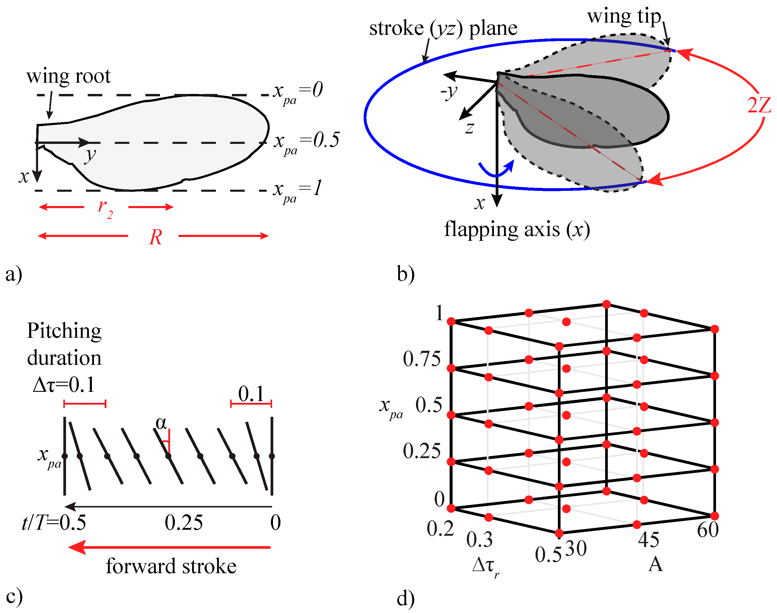
2.1. Case Setup and Wing Kinematics

We consider hovering flight for rigid wings. The Reynolds number is Re = ρUc/µ, where ρ is the constant air density, U is a reference velocity, c is the mean wing chord, and µ is the dynamic viscosity. In this study, the Reynolds number is kept constant at Re = 100, relevant to a fruit fly flight [6,9,12,16,26]. The reference velocity U is the maximum flapping velocity at the spanwise location of the center of the second moment of wing area r₂ [31], i.e., U = 2πfZ${\hat{r}}_2$R, where f is the stroke frequency, Z is the half peak-to-peak stroke amplitude, and ${\hat{r}}_2$ = 0.57 is the spanwise location of the center of the second moment of wing area, normalized by the wing length R. The aspect ratio AR = R/c = 3.02 was determined by using an actual fruit fly wing to create a 3D model as shown in Section 2.2.2. With the Reynolds number held constant at 100, the stroke frequency f and amplitude Z are dependent on each other. The reduced frequency is defined as k = 2πfc/(2U) = (2Z${\hat{r}}_2$AR)⁻¹. For this study, the stroke amplitude is kept constant at Z = 49.3°, so that the reduced frequency is applicable to a fruit fly flight k = 0.33 [3].

For hovering flight for insects, there are two primary kinematics: flapping and pitching. In this study, the flapping motion is assigned a sinusoidal rotation about the wing root as

$$\mathsf{\zeta }\left(t/T\right)=\mathrm{Zcos}\left(2\mathsf{\pi }t/T\right),$$

(1)

where t/T is the non-dimensional time, the time t normalized by the flapping period T = 1/f. A schematic of the 3D flap motion is shown in Figure 1.

The pitching motion considered in this study is motivated by the work by Sun and co-workers [11,12] as

$$\alpha (t/T)=\{\begin{array}{cc}{\alpha }_d+\frac{\mathrm{A}}{\mathsf{\Delta }{\tau }_r}\left\{\left(\frac{t}{T}-{\tau }_1\right)-\frac{\mathsf{\Delta }{\tau }_r}{2\pi }\sin \left[\frac{2\pi }{\mathsf{\Delta }{\tau }_r}\left(\frac{t}{T}-{\tau }_1\right)\right]\right\}\hfill & \mathrm{for}\frac{t}{T}\le {\tau }_1\\ {\alpha }_d-\frac{\mathrm{A}}{\mathsf{\Delta }{\tau }_r}\left\{\left(\frac{t}{T}-{\tau }_2\right)-\frac{\mathsf{\Delta }{\tau }_r}{2\pi }\sin \left[\frac{2\pi }{\mathsf{\Delta }{\tau }_r}\left(\frac{t}{T}-{\tau }_2\right)\right]\right\}\hfill & \mathrm{for}{\tau }_2\le \frac{t}{T}\le {\tau }_2+\mathsf{\Delta }{\tau }_r\\ {\alpha }_u+\frac{\mathrm{A}}{\mathsf{\Delta }{\tau }_r}\left\{\left(\frac{t}{T}-{\tau }_3\right)-\frac{\mathsf{\Delta }{\tau }_r}{2\pi }\sin \left[\frac{2\pi }{\mathsf{\Delta }{\tau }_r}\left(\frac{t}{T}-{\tau }_3\right)\right]\right\}\hfill & \mathrm{for}\frac{t}{T}\ge {\tau }_3\end{array}$$

(2)

where A is the pitch amplitude and α_d and α_u are the forward and return pitch amplitudes, respectively. In this study the pitch amplitude is A = α_d = α_u. The parameter Δτ_r is a non-dimensional number that determines the duration of the pitch rotation in terms of the period. When the pitching duration is small the pitching motion is rapid and is confined to the end of each stroke. When the pitching duration is Δτ_r = 0.5, the pitching motion is as slow as it can be because it lasts the entire stroke. Depending on Δτ_r, the duration of the pitch the pitching waveform can vary from sinusoidal (Δτ_r = 0.5) to a square wave when Δτ_r approaches 0. The parameters τ₁, τ₂, and τ₃ determine the timing of the rotation. Since only symmetric rotation is considered in this study_, τ₁ = Δτ_r/2, τ₂ = τ₁ + Δτ_r/2, and τ₃ = 0.5 − Δτ_r/2. The pitching motion is imposed on the pitch axis location x_pa, which is normalized by c and measured from the leading edge. When x_pa = 0.0, the pitch axis is at the leading edge and when x_pa = 1 the pitch axis is at the trailing edge. Figure 1b shows a diagram of the pitching motion for a half-stroke for A = 45°, x_pa = 0.5, and Δτ_r = 0.2.

We vary three pitching parameters to compare the performance of the quasi-steady model and Navier–Stokes equation solvers. The three independent variables are the pitching amplitude A = 30°, 45°, 60°, the location of the pitching axis measured from the leading edge, normalized by the chord x_pa = 0, 0.25, 0.5, 0.75, 1, and the duration of the pitch Δτ_r = 0.2, 0.3, 0.5. The study focuses on the pitching kinematics because the angle of attack has been shown to greatly affect the aerodynamic performance [4]. There are 45 combinations for these values, which are simulated for each of the aerodynamic models. A case by case breakdown for all 45 cases is shown in Figure 1d and

Table A1. Cases considered in this study.

Case	α (°)	Δτr	xpa	Case	α (°)	Δτr	xpa	Case	α (°)	Δτr	xpa
1	30	0.2	0	16	30	0.5	0.25	31	30	0.3	0.75
2	45	0.2	0	17	45	0.5	0.25	32	45	0.3	0.75
3	60	0.2	0	18	60	0.5	0.25	33	60	0.3	0.75
4	30	0.3	0	19	30	0.2	0.5	34	30	0.5	0.75
5	45	0.3	0	20	45	0.2	0.5	35	45	0.5	0.75
6	60	0.3	0	21	60	0.2	0.5	36	60	0.5	0.75
7	30	0.5	0	22	30	0.3	0.5	37	30	0.2	1
8	45	0.5	0	23	45	0.3	0.5	38	45	0.2	1
9	60	0.5	0	24	60	0.3	0.5	39	60	0.2	1
10	30	0.2	0.25	25	30	0.5	0.5	40	30	0.3	1
11	45	0.2	0.25	26	45	0.5	0.5	41	45	0.3	1
12	60	0.2	0.25	27	60	0.5	0.5	42	60	0.3	1
13	30	0.3	0.25	28	30	0.2	0.75	43	30	0.5	1
14	45	0.3	0.25	29	45	0.2	0.75	44	45	0.5	1
15	60	0.3	0.25	30	60	0.2	0.75	45	60	0.5	1

in Appendix A.

2.2. Aerodynamic Models

The forces and moments generated by the flow over the wings are the most significant source of forces for a flapping flyer. We consider two different models for the aerodynamic forces:

• A quasi-steady model from Sane and Dickinson [8,18,30],
• A 3D Navier–Stokes equations solution of the rigid wing motion.

The details of the employed quasi-steady model and the Navier–Stokes equation solver are described by Bluman, Sridhar, and Kang [32] and summarized in the following subsections. The results of the model are presented in terms of coefficients of lift C_L, drag C_D, and moment about the pitching axis (C_M), defined as

$$C_L=\frac{L}{\frac{1}{2}\rho U^{2}Rc},C_D=\frac{D}{\frac{1}{2}\rho U^{2}Rc},C_M=\frac{M}{\frac{1}{2}\rho U^{2}R{c}^2}$$

(3)

where L, D, and M are the cycle-averaged lift, drag, and moment about the pitching axis, respectively.

2.2.1. Quasi-Steady Aerodynamic Model

In order to provide comparisons among the various flight dynamics studies that have used the Sane and Dickinson model [18] extensively in the past, the same model will be incorporated into this study as well. Their model, which is derived from blade element analysis, attempts to capture the quasi-steady contributions of translational lift F_trans, rotational lift from circulation F_rot, and added mass force F_a, to the aerodynamic force on the wing. Additional forces generated via wake capture are omitted from the model.

The translational lift and drag coefficients are provided by fitting an expression to experimental results for a range of angles of attack: AoA = −10° to 90°, resulting in Equation (4), where u_t is the wing’s instantaneous velocity.

$$F_{trans}=\left|\begin{array}{c}{L}_{trans}\\ D_{trans}\end{array}\right|=\frac{1}{2}\rho u_t^{2}Rc\left|\begin{array}{c}0.225+1.58\sin \left(2.13AoA-7.2\right)\\ 1.92-1.55\cos \left(2.04AoA-9.82\right)\end{array}\right|$$

(4)

The rotational force is developed by the wing’s rotation imparting additional circulation to the flow, which can enhance lift. In this study, we use Equation (5), an expression equivalent to that provided by Sane and Dickinson [18]. In Equation (5), ${\hat{r}}_1$ is the spanwise location of the center of the first moment, normalized by the wing length and $\hat{v}$ is the virtual mass. Ellington [15] provides expressions for the terms $\hat{v}$ and ${\hat{r}}_1$, which are a function of the wing shape, and also cataloged their values for several insects. The expressions are provided in Equation (6) for convenience, where $\hat{r}$ is the spanwise coordinate, normalized by R and $\hat{c}$ is the chord at a spanwise location, normalized by c. We use the average values given by Ellington [15] for fruit flies in the present study of $\hat{v}$ = 1.0 and ${\hat{r}}_1$ = 0.49.

$$F_{rot}=-C_{rot}\left(\frac{3}{4}-x_{pa}\right)\rho \left|u_t\right|\dot{\alpha }{c}^{2}R\widehat{v}{\widehat{r}}_1$$

(5)

$$\widehat{v}{\widehat{r}}_1={{\displaystyle \int }}_0^1{\widehat{c}}^2\widehat{r}d\widehat{r}\mathrm{and}\widehat{v}={{\displaystyle \int }}_0^1{\widehat{c}}^{2}d\widehat{r}$$

(6)

The theoretical value for C_rot is C_rot = C_rot,theo = π [18]. However, Sane and Dickinson [18] show that C_rot depends on the nondimensional rotational velocity $\widehat{\mathsf{\omega }}$ = ωc/U_tip, where ω is the absolute angular velocity of the wing about its pitch axis and U_tip is the reference velocity at the wing tip. Based on their experiments, an empirical fit was proposed as C_rot = C_rot,exp = (−11.77$\widehat{\mathsf{\omega }}$ + 0.8152)(0.75 − x_pa). In this study, we use C_rot,exp to calculate the rotational force and quantify its benefit by comparing the resulting force against the values obtained with C_rot,theo in Section 3.

Sane and Dickinson’s added mass term, accounting for differing pitch axis locations as per Leishman [12] and Babinsky [13], is

$$F_a=\pi \rho R{c}^2\left\{\frac{{\widehat{r}}_2}{4}\left(\ddot{\zeta }\sin AoA+\dot{\zeta }\dot{\alpha }\cos AoA\right)\widehat{v}{\widehat{r}}_1-\ddot{\alpha }\frac{c}{8}\left(x_{pa}-\frac{1}{2}\right)\widehat{v}\right\}.$$

(7)

The aerodynamic moment about any point can be determined as long as the point of application for each aerodynamic force is known. The circulatory force terms, i.e., F_trans and F_rot, are applied at the quarter chord, although these assumptions may be over-simplified as recent studies [27,33] have shed more light on the location of the center of pressure in flapping wing motions. There is a residual pitching moment that arises due to wing rotation given by Leishman [34], which is

$$M_{circ}=\frac{\pi }{4}\rho c^3{u}_t\left(x_{pa}+\frac{1}{2}\right)\dot{\alpha }.$$

(8)

The increment in lift due to added mass is taken to act at the mid-chord. Additionally, Fung [35] demonstrates that a nose down couple is generated by the pitch acceleration as

$$M_a=-\frac{\pi \rho }{8}{\left(\frac{c}{2}\right)}^4\ddot{\alpha }.$$

(9)

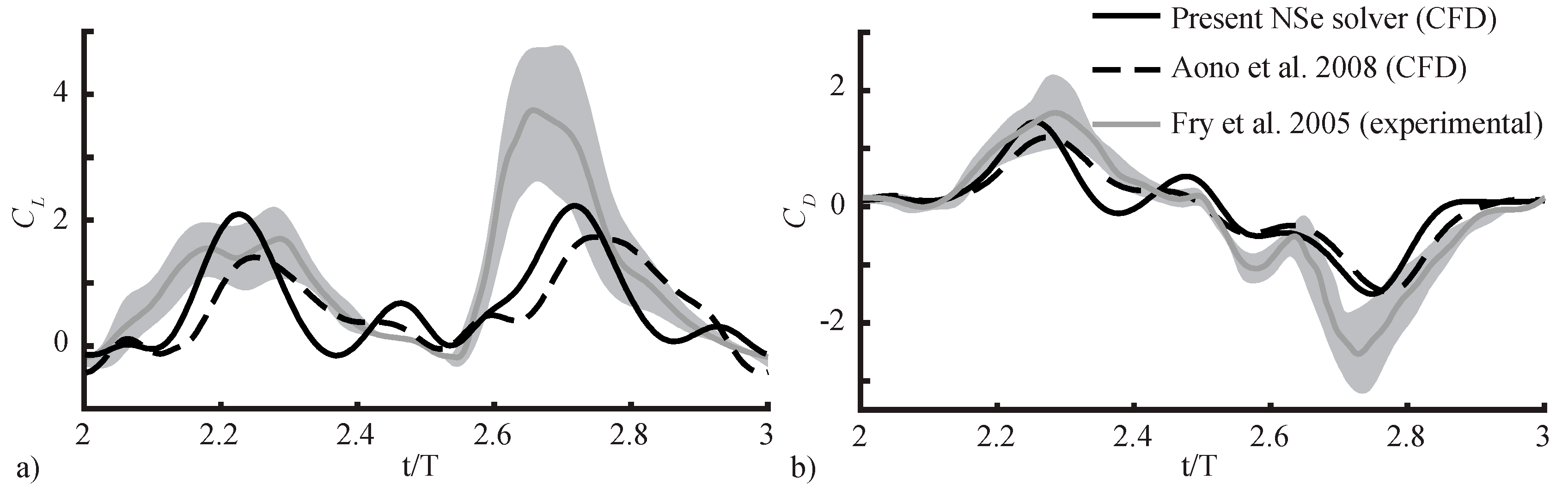
2.2.2. Navier–Stokes Equation Model

To provide high fidelity solutions to the Navier–Stokes equations, the flow around the wing is modeled using a well-validated Navier–Stokes equation solver. The case setup for hovering flight requires the kinematics of the wing as described in Section 2.1 to be imposed on a quiescent fluid. The fluid response and resulting viscous and pressure distributions on the body are described by the unsteady, incompressible Navier–Stokes equations given as

$$\begin{gathered} {\nabla }^{*}\cdot {\mathrm{V}}^{*}=0 \\ \frac{k}{\pi }\frac{\partial {\mathrm{V}}^{*}}{\partial t^{*}}+\left({\mathrm{V}}^{*}\cdot {\nabla }^{*}\right){\mathrm{V}}^{*}=-{\nabla }^{*}p+\frac{1}{Re}{\mathsf{\Delta }}^{*}{\mathrm{V}}^{*} \end{gathered}$$

(10)

where the asterisk (*) indicates variables that have been non-dimensionalized with the reference velocity U, the flapping frequency f, and the mean wing chord c. These equations are solved in three dimensions using a structured, finite-volume, pressure-based incompressible Navier–Stokes equation solver used extensively in flapping wing studies in the past. For example, Teng et al. [36] and Shyy et al. [37] used the solver for Re = O(10²), similar to the present study. Additionally, Lian et al. [38] and Kamakoti and Shyy [39] used it for Re = O(10⁴). Appendix B demonstrates low Re motion being simulated with sufficient accuracy.

The 3D grid is a structured, rectangular grid composed of eight separate blocks that is modeled to have geometry similar to a fruit fly wing. There are 15 cells along the tip and root of the wing, 53 cells along the leading and trailing edges, and cells approaching the wing are constrained to be only 0.01c apart. The outer boundary of the domain is located approximately 30 chord lengths from the wing. The wing is infinitely thin. Figure 2 shows the fruit fly wing used to develop the 3D grid. The boundary conditions are no-slip on the surface of the wing and extrapolated pressure at the boundary. The initial conditions are quiescent flow. The wing is rigidly moved at each time step in accordance with the prescribed wing kinematics.

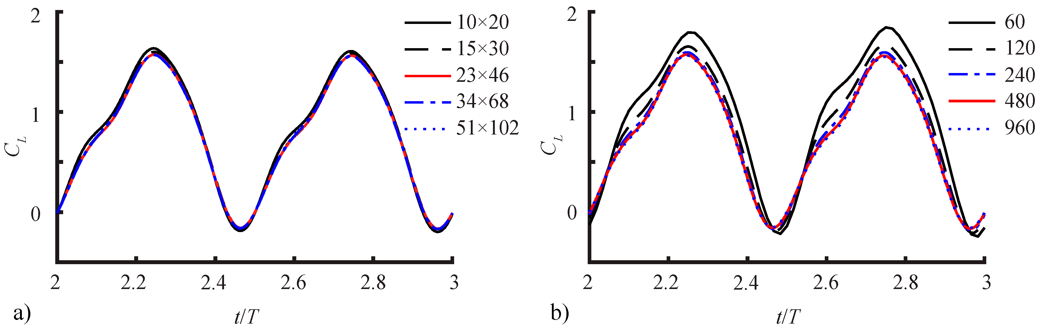
2.2.3. Spatial and Temporal Sensitivity Study

The number of nodes around the wing is systematically increased with each grid in the spatial sensitivity study and the number of time steps was increased for each case in the temporal sensitivity study. These studies are conducted on the baseline kinematics with h_a = 1.5, Δτ_r = 0.5, x_pa = 0.5, α_d = α_u = 45° (case 26 in Table A1). The medium grid (23 × 46 × 92) with 631,800 number of cells and 480 time steps per period yields sufficiently converged solution for lift as shown in Figure 3 and

Table 1. Spatial and temporal sensitivity for 3D grids. Five different meshes and five timestep sizes were included in the spatial and temporal sensitivity study. The medium grid (23 × 46 × 92) with 631,800 cells was chosen with 480 timesteps/period for the NSe simulations.

	Cells	Timesteps/Period	Total Cells	<CL>	L1-Norm	L2-Norm
spatial	10 × 20 × 40	480	46,930	0.7820	0.0518	0.0571
	15 × 30 × 60	480	168,200	0.7667	0.0220	0.0257
	23 × 46 × 92	480	631,800	0.7543	0.0113	0.0152
	34 × 68 × 136	480	2,091,874	0.7543	0.0075	0.0094
	51 × 102 × 204	480	7,181,504	0.7574	---	---
temporal	23 × 46 × 92	60	631,800	1.0504	0.1243	0.2990
	23 × 46 × 92	120	631,800	0.8705	0.1071	0.1830
	23 × 46 × 92	240	631,800	0.7874	0.0848	0.1032
	23 × 46 × 92	480	631,800	0.7543	0.0519	0.0448
	23 × 46 × 92	960	631,800	0.7336	---	---

.

3. Results and Discussion

3.1. Aerodynamic Response under the Three-Dimensional Pitch-Flap Motion

Before comparing the performance of the QS model in Section 3.2, we first assess the aerodynamic response from the NSe solution. In particular, we investigate how the three design variables x_pa, A, and Δτ_r affect the resulting C_L, C_D, and C_M under the 3D pitch-flap motion given by Equations (1) and (2).

Figure 4 shows C_L in the design space of x_pa, A, and Δτ_r. The middle pitching amplitude α = 45° has the largest C_L at x_pa = 0 and Δτ_r = 0.2 (rapid rotation). For x_pa > 0.5, larger lift is seen at lower A and, therefore, at higher AoAs (AoA is roughly 90°–α). When the pitching axis is close to the leading edge, a longer pitching duration reduces lift. On the other hand, when x_pa > 0.5, the lift is nearly insensitive to Δτ_r. The effects of the pitching duration are the most noticeable when the pitch axis is near the trailing edge at A = 60°. The lowest lift is found in this region when A = 60°, x_pa = 1, and Δτ_r = 0.2.

The global trends in Figure 4 suggest that the extreme pitching kinematics, i.e., the motion where the pitching amplitude is large A ≥ 45°, the duration is short Δτ_r < 0.3, and the pitching axis is at the leading or trailing edge have the most effect on the lift coefficient. On the other hand, the lift response is mild when the pitch axis is at the midchord x_pa = 0.5 and the duration is relatively long Δτ_r ≥ 0.3. To analyze the flapping wing physics further, we consider three parametric studies where a single design parameter is changed at extreme and mild motions as summarized in

Table 2. Extreme and mild cases considered.

A	Δτr	xpa	Pitching Motion
30°, 45°, 60°	0.3	0.5	Mild
30°, 45°, 60°	0.2	1.0	Extreme
30°	0.2, 0.3, 0.5	0.5	Mild
60°	0.2, 0.3, 0.5	1.0	Extreme
30°	0.3	0.0, 0.25, 0.5, 0.75, 1.0	Mild
60°	0.2	0.0, 0.25, 0.5, 0.75, 1.0	Extreme

.

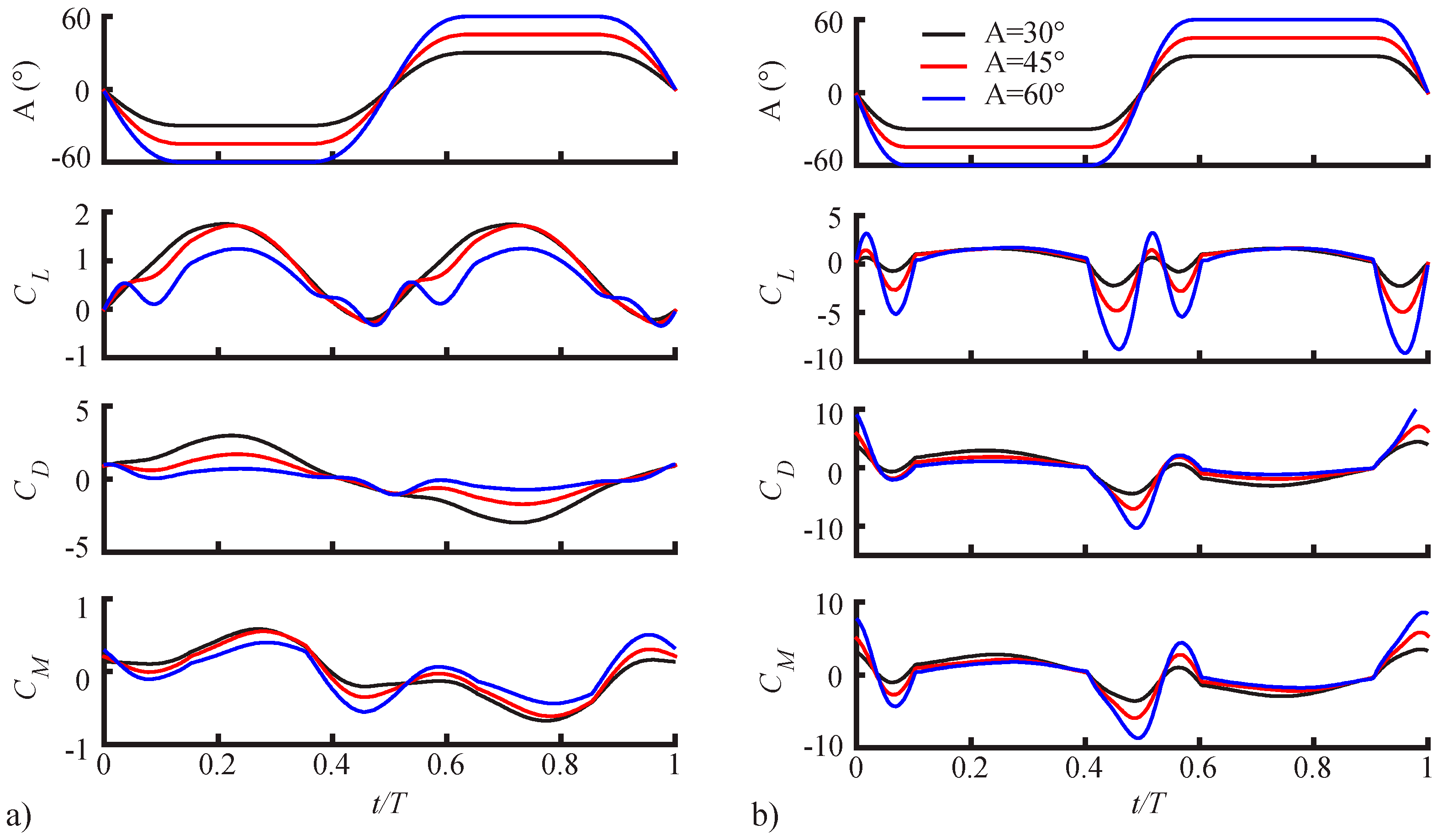
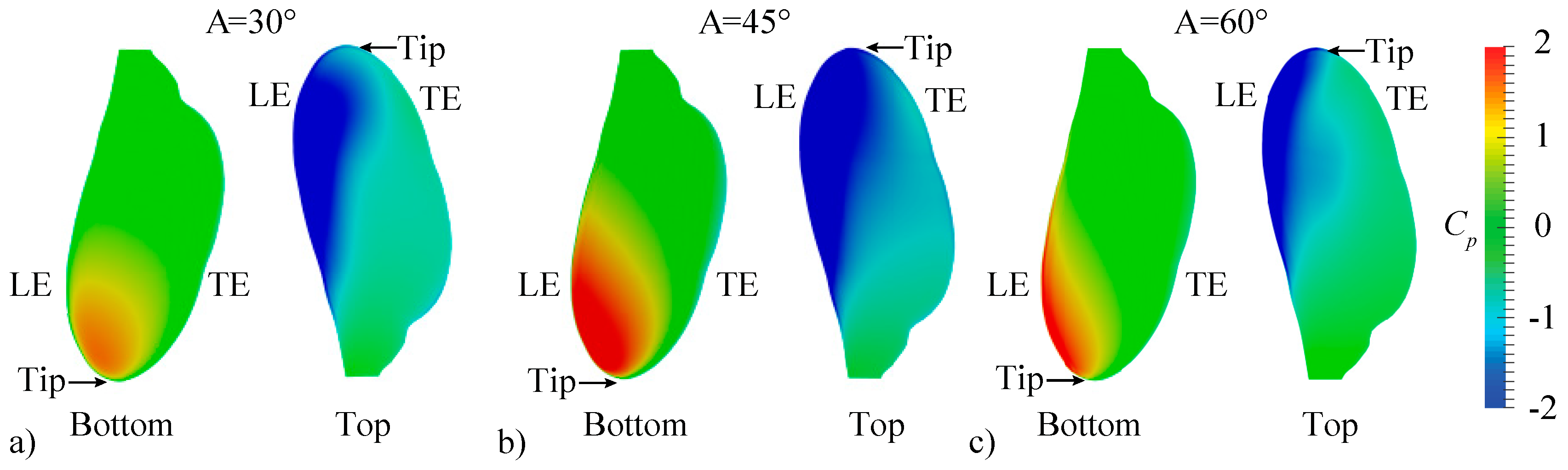
3.1.1. Pitching Amplitude Trends

Time histories of the aerodynamic forces and moment about the pitching axis over a full cycle are shown in Figure 5. The pitching amplitude is changed from 30 to 60°. Figure 5a shows modest forces result with Δτ_r = 0.3 and x_pa = 0.5. Figure 5b shows a case with extreme pitching motion with kinematics Δτ_r = 0.2 and x_pa = 1.0.

Both forward and return strokes generate similar lift profiles. The pitching occurs at the beginning and end of the stroke. The angle of attack is held constant during the mid-stroke. At the beginning and end of each stroke, we see an increase in the magnitude for the peaks and valleys for lift coefficient as the pitching amplitude increases.

For the mild motions in Figure 5a, the change in A mostly affects the magnitude of the aerodynamic forces during the mid-stroke, where the flapping velocities are the highest. The pitching at the ends of the strokes are relatively slow, resulting in rotational peaks that are relatively smaller. At the middle of the stroke (t/T = 0.25) the smallest lift coefficient is seen at A = 60° with A = 45° and A = 30° having similar values. In Figure 5b, on the other hand, the extreme motions with rapid pitching (shorter pitch duration Δτ_r and pitch axis x_pa at the trailing edge) show the lift coefficient has much larger peaks during the ends of the strokes than seen in the less extreme case in Figure 5a. The difference in the lift during the midstroke is much smaller than during the ends of the strokes.

The drag coefficient shows similar trends as the lift coefficient. The peak values for the drag coefficient are seen at the areas of pitching with the rapid pitching case shown in Figure 5b, yielding much larger drag. However, at the middle of the stroke, we see the largest drag comes from pitching amplitude A = 30° with decreasing drag coefficient as pitching amplitude increases. The largest drag is found at A = 30° because the wing is more vertical during the midstroke compared to higher pitching amplitudes. The moment coefficient about the pitching axis is closely related to the lift and drag, which is also what we observe.

Figure 6 shows the iso-surfaces for the Q-criterion (Q = 0.75) for the forward stroke with A = 30° to A = 60° for the mild motions. The Q-criterion is an invariant of the velocity gradient tensor, defined as

$$Q=-\frac{1}{2}\frac{\partial u_i}{\partial x_j}\frac{\partial u_j}{\partial x_i}.$$

(11)

The Q-isosurfaces provides a visual indication of the vortical structures in the flow field [40].

Larger vortical structures are produced when the wing is pitching at a lower amplitude (A = 30°), since the angle of attack is the highest during the mid-stroke. When the pitching amplitude is high (A = 60°), the vortices are relatively smaller. The Q-isosurfaces are similar in structure for when A = 45° and A = 30°, where we see larger vortices around the leading edge, trailing edge, and wing tip, also indicated by the similarity in the lift coefficient in Figure 5a.

At t/T = 0.5, wing tip vortices move up over the wing. This spanwise non-uniformity is also seen in Figure 7, which shows the contour plots of the coefficient of pressure for the forward stroke of the same mild cases for the top and bottom of the wing. Very large pressure coefficient areas are observed near the wing tip, consistent with the highest flapping wing velocity magnitude towards the wing tip. These results suggest that most of the lift is produced near the wing tip.

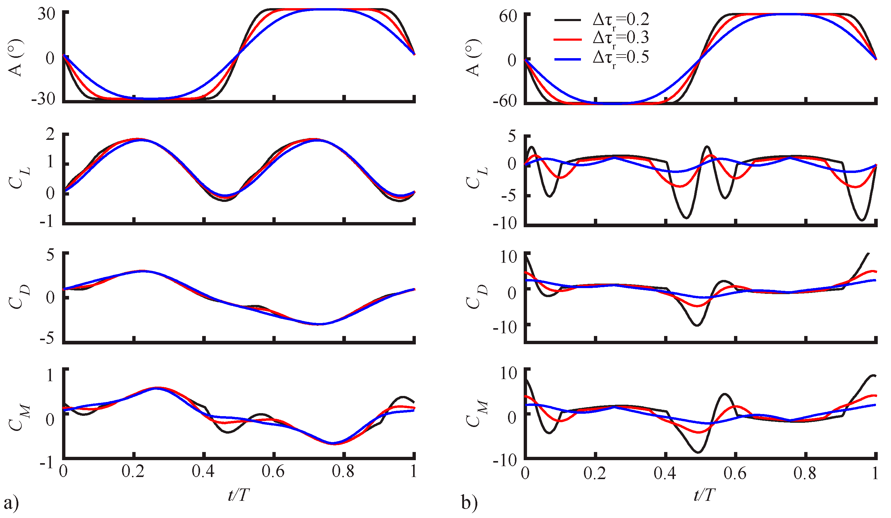
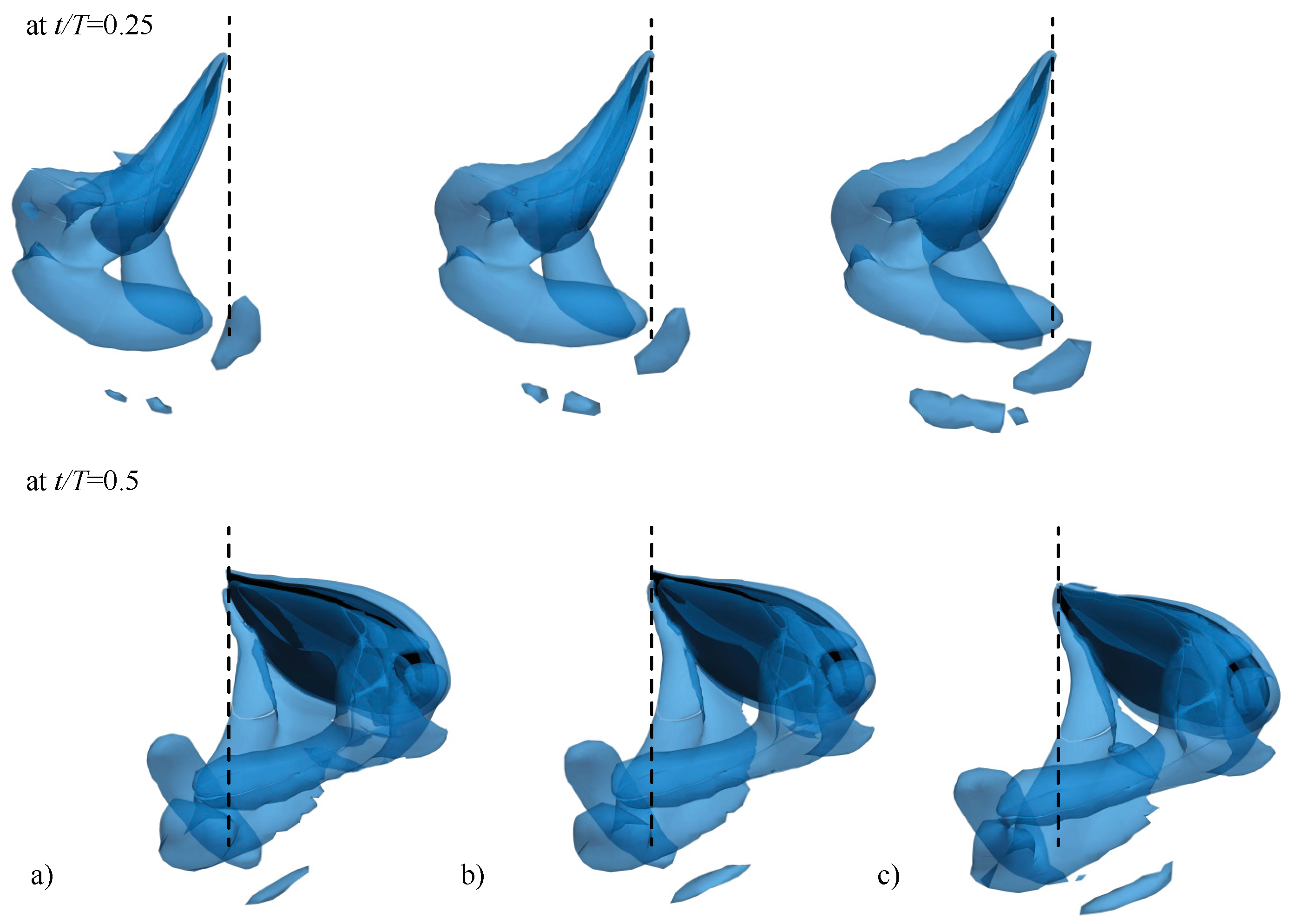
3.1.2. Pitching Duration Trends

A comparison of the aerodynamic forces and moment about the pitch axis is shown in Figure 8 for the three pitching durations for the mild and extreme pitching motions. A pitching duration of Δτ_r = 0.5 implies that the pitching takes place over the entire stroke. As the pitching duration shortens, i.e., as the wing pitches faster, the lift coefficient at the beginning and end of the stroke shows larger peaks in Figure 8a. Then at the middle of the stroke (t/T = 0.25) the lift coefficient has similar magnitudes. This trend is magnified for the rapid pitch extreme motions in Figure 8b with much larger lift peaks. The drag and moment coefficients show similar trends as the lift coefficient.

The similarity between the iso-Q-surfaces shown in Figure 9 with different pitching durations is striking at the midstroke. At the end of the stroke, the shortest pitching duration Δτ_r = 0.2 shows slightly larger iso-Q-surface. The larger vortical structures at the stroke ends due to quicker rotation are consistent with the higher force magnitudes in Figure 8.

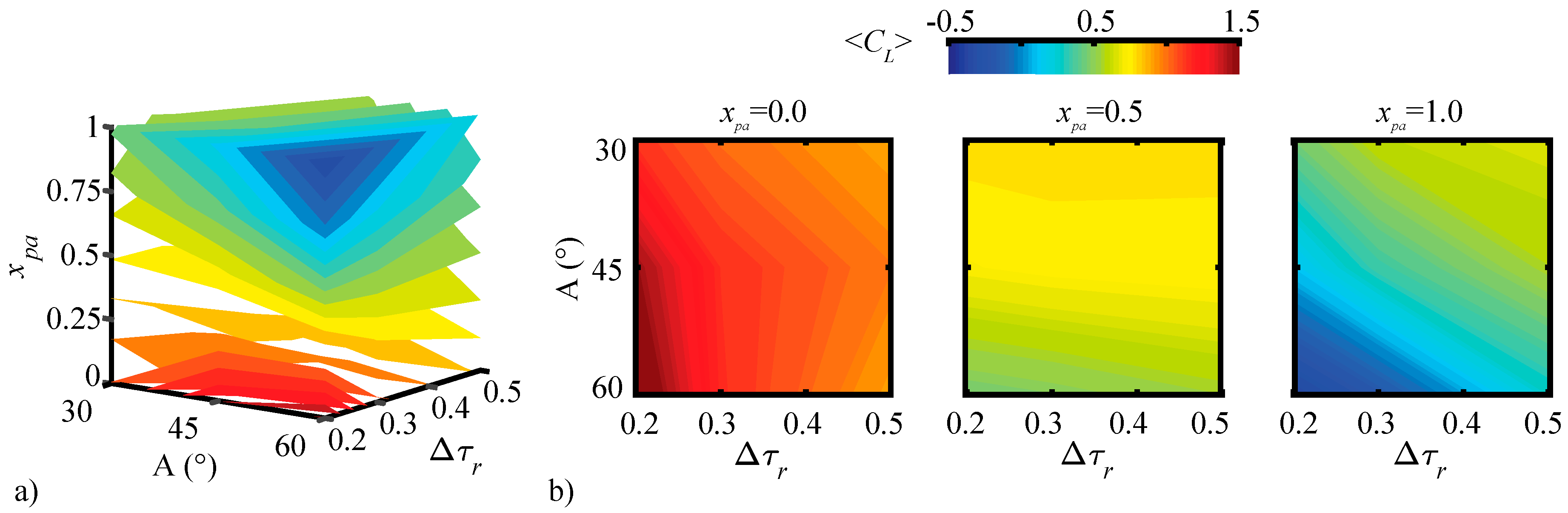
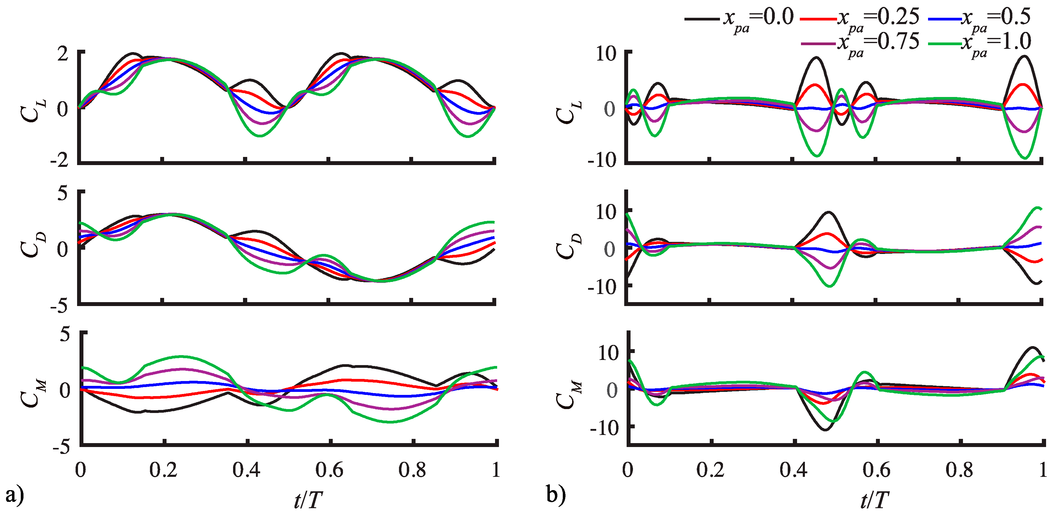
3.1.3. Pitching Axis Trends

Figure 10 show the aerodynamic forces and moment about the pitching axis, where the pitching axis is changed from the leading edge, x_pa = 0.0, to the trailing edge, x_pa = 1.0. Figure 10a shows a case with a relatively small pitching motion with A = 30° and Δτ_r = 0.3. Figure 10b shows a case with large, rapid pitching motion with A = 60° and Δτ_r = 0.2.

In Figure 10a the lift coefficient at the beginning of the stroke increases as the pitch axis location moves towards the trailing edge. At the end of the stroke, this trend reverses. During the middle of the stroke (t/T = 0.25), the lift coefficient has similar values. These trends are similar in the extreme cases in Figure 10b with the magnitudes magnified. The difference in lift coefficient is much smaller between different pitching axis when the pitching motion is small (Figure 10a) and the difference is large when the pitching kinematics are extreme (Figure 10b). The drag and moment coefficients show similar trends as the lift coefficient.

The iso-Q-surfaces are generally similar as shown in Figure 11. Key differences can be seen at t/T = 0.0 in the LEVs. For trailing edge pitching axis, a large LEV has formed across most of the span (Figure 11c). When the pitching axis is at the leading edge (Figure 11a), the LEV spins in the opposite direction, still covering most of the span. For x_pa = 0.5, the leading-edge vortex is much smaller and can be found only near the wing tip (Figure 11b). Also, as the pitching axis moves from the leading edge to trailing edge, the wingtip vortex becomes stronger. The reverse is true for the wing root vortex, which is larger when pitching axis is at the leading edge.

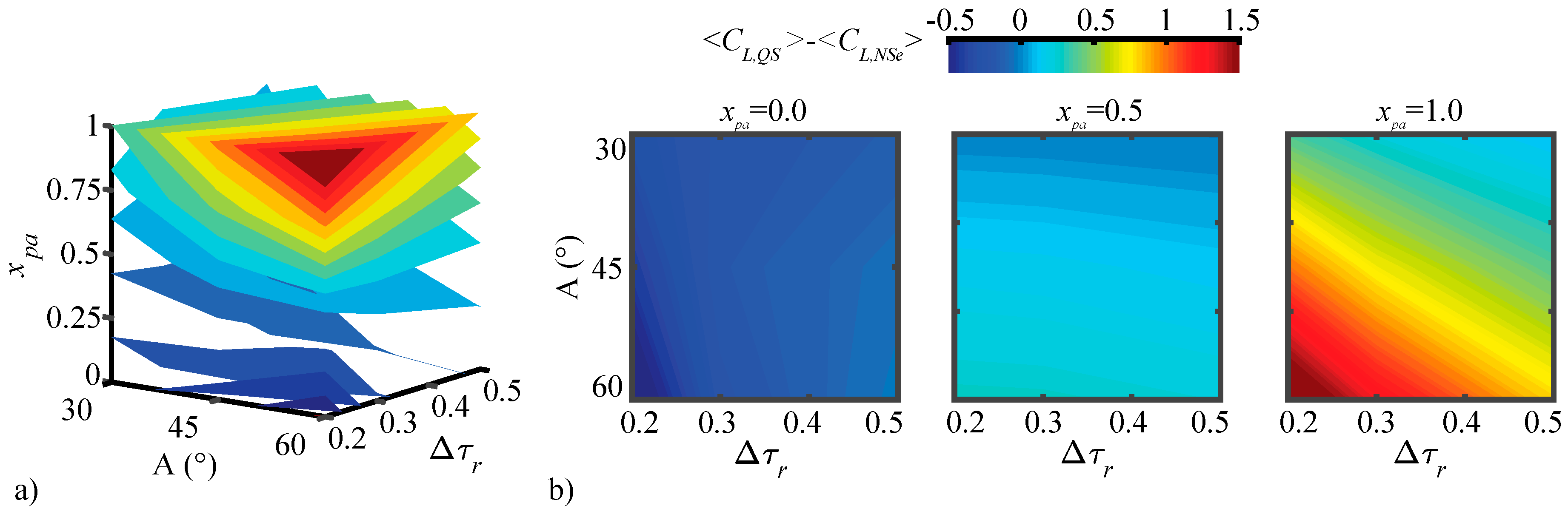
3.2. Assessment of the QS Model

Analysis of the aerodynamic response due to the changes in the three design variables in Section 3.1 indicates that the force magnitudes during the midstroke are affected primarily by the pitching amplitude A, whereas the forces at the ends of the strokes are influenced by all three design variables. Furthermore, there are two main regions worth noting in the design space. The first is where the pitching kinematics are mild, i.e., the pitching amplitude is small, the duration is long, and the pitching axis is located near the mid-chord. In this area, the sensitivity of the aerodynamic response is relatively mild. The second area is where the pitching kinematics are extreme, the amplitude is large, the duration is short, and the pitching axis is away from mid-chord typically towards the trailing edge. Also, when x_pa is away from 0.5, either the leading edge (LE) or trailing edge (TE) will experience the largest velocity due to rotation. For symmetric rotations, which we employ in this study, the LE will experience a greater relative flow velocity when x_pa = 1 then vice versa, because the LE rotates into the flow, whereas the TE rotates away from the flow.

Figure 12 shows the absolute difference between the cycle-averaged lift coefficients between the QS and NSe results in the design space. Three general trends can be noticed. Firstly, as the pitching axis moves away from mid-chord the differences tend to increase. The largest differences are seen at x_pa = 1.0, with the smallest typically being at x_pa = 0.5 or x_pa = 0.25. Secondly, as the pitching amplitude increases we see an increase in differences in cycle-averaged lift coefficient. Thirdly, a longer pitching duration leads to a smaller difference in cycle-averaged lift coefficient.

We discuss the qualitative differences by focusing on the motion with the largest difference and the motion with the smallest difference. A comparison of the wing kinematics between these two cases is found in Figure 13. To analyze the differences between the two methods we look at one full stroke of each case in order to capture the asymmetry of the force coefficients in the Navier–Stokes solutions. The asymmetry in the NSe force coefficients are due to the nonlinear wing-wake interaction, which cannot be modeled by a QS model, and the asymmetry in the initial direction of the flapping motion, i.e., forward versus backward strokes [41]. Recall that the NSe solutions are taken from the third flapping cycle, as described in Section 2.2.3.

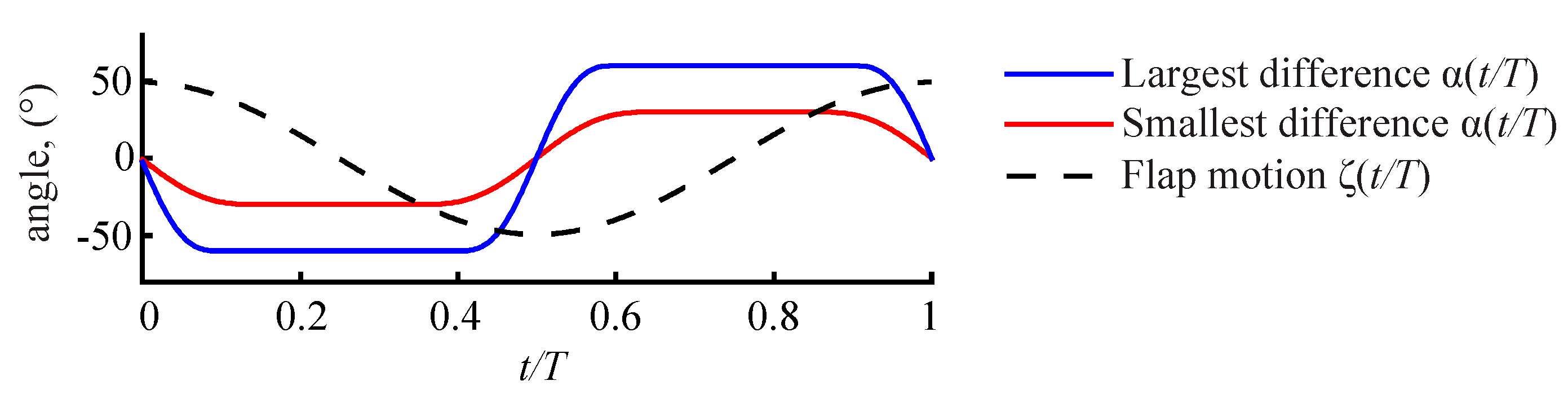
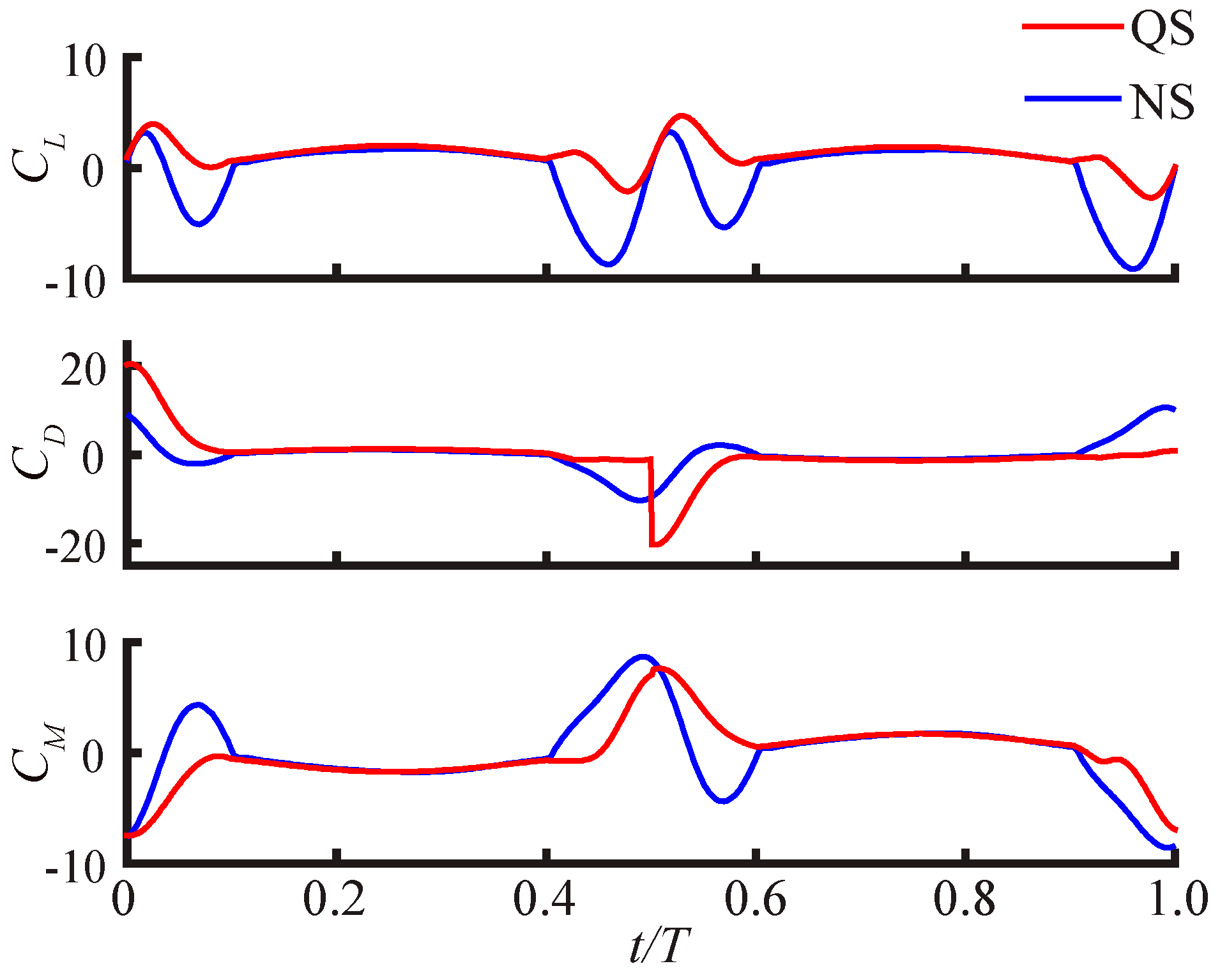
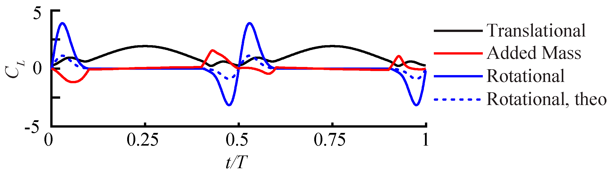
3.2.1. Largest Difference Motion: Case 39

The largest difference in the cycle-averaged lift coefficients between the models, which is 1.7, occurs when the kinematics are extreme: x_pa = 1.0, A = 60°, and Δτ_r = 0.2. The NSe model predicts a lift coefficient of −0.59, whereas the QS model overpredicts the lift coefficient as 1.11.

We plot the direct comparison of lift, drag, and moment coefficient for the case with largest differences in Figure 14. The general trends are similar. Both models predict large peaks and valleys for all three coefficients at the beginning and end of the strokes where the pitching motion occurs. At the mid-stroke, where the angles of attacks are held constant, much smaller coefficients are predicted than during the pitching motion.

Figure 15 shows a breakout of the components of lift for the QS model in terms of the translational, rotational, and added mass components (Equations (4)–(9)). The lift coefficient can be divided into three major areas based on the pitching duration: (i) beginning of the forwards stroke (0.0 < t/T < 0.1), (ii) middle of forward stroke (0.1 < t/T < 0.4), and (iii) end of forward stroke (0.4 < t/T < 0.5).

The first interval starts at the beginning of the forward stroke and ends when the first part of the pitching motion stops and the pitching angle is held constant at A = 60°. This portion of the stroke is dominated by the rotational component of lift, due to the large pitching amplitude and short pitching duration. The translational velocity is still relatively slow and, therefore, the translational lift component much smaller. The translational component has a small peak due to the pitching axis being at the trailing edge, which means the wing is rotating in the direction of the flapping motion. In the second portion of the stroke, the translational component of lift dominates. Both the rotational and added mass contributions vanish due to the constant pitch angle. The translational component peaks at the midstroke, where the flapping velocity is the highest. The QS solution agrees well with the NSe results. In the third interval, the trends are similar as in the first interval. The signs of the rotational and added mass contributions are opposite, because of the pitch up motion. As the wing rapidly pitches up while decelerating, negative lift is generated. The QS model predicts an increase in lift coefficient and then drops off. The NSe model predicts the lift coefficient to decrease as soon as the pitching begins at t/T = 0.4.

The major differences in the lift coefficient occur during the rapid pitch motion where the rotational component is dominant. A phase shift and a difference in magnitude is observed, suggesting that the rotational term in the quasi-steady model is not accurate for the considered kinematics. Note that the use of the theoretical rotational lift coefficient C_rot,theo = π worsens the accuracy significantly during this portion of the stroke. This significant inaccuracy is likely due to the fact that the empirical terms in the Sane and Dickenson QS model [18] are obtained for x_pa ≤ 0.66, where the present study considers x_pa ≤ 1. In addition to this assumption, the range of dimensionless rotational velocity ($\hat{\mathsf{\omega }}$ in C_rot of Equation (5)) ranges from 0.166 to 0.374 in Sane and Dickinson’s QS formulation [18]. However, the present study includes a range of $\hat{\mathsf{\omega }}$ between 0.5 and 1.75 (which is close to the range typical of insects [16]), resulting in values completely outside that used by Sane and Dickinson [18]. Considering the fact that the rotational velocity scales the rotational forces quadratically, it is unsurprising that this term creates large discrepancies between models, especially at such high values. Additionally, a more accurate rotational drag term could be used in the model, such as the formulations presented in recent studies [27,28]. Since the rotational drag term is highly dependent on the rotational axis, it is expected that improved accuracy would rectify the differences between the QS and NSe solutions even at more extreme pitch axis locations.

Similar to the lift, the drag peaks during the pitching motion and the drag magnitude significantly reduces during the middle of the stroke. It is important to notice the magnitude of the peak drag. The rapid pitching of the wing in the direction of the flapping motion with x_pa = 1.0 results in a large drag force being produced, overpredicting the NSe solutions significantly. At the beginning of the forward stroke, the drag is almost equally composed of the translational and rotational components. Based on the lift comparison, we argue that the inaccuracy of the rotational lift causes the large difference observed in this interval. As the pitching ends, the pitching angle is constant and the drag is made up entirely of the translational component. A closer agreement exists in this phase.

Figure 14 shows that the moment coefficient has large peaks and valleys during the pitching and smaller ones for the middle of the stroke. The close agreement in the first portion of the stroke may be due to a cancellation of errors in the lift and drag coefficients. The moment coefficients are close to zero during the second interval, well predicted by the QS model. However, large discrepancies are noticeable in the final interval, consistent with the observed differences in the force coefficient comparisons.

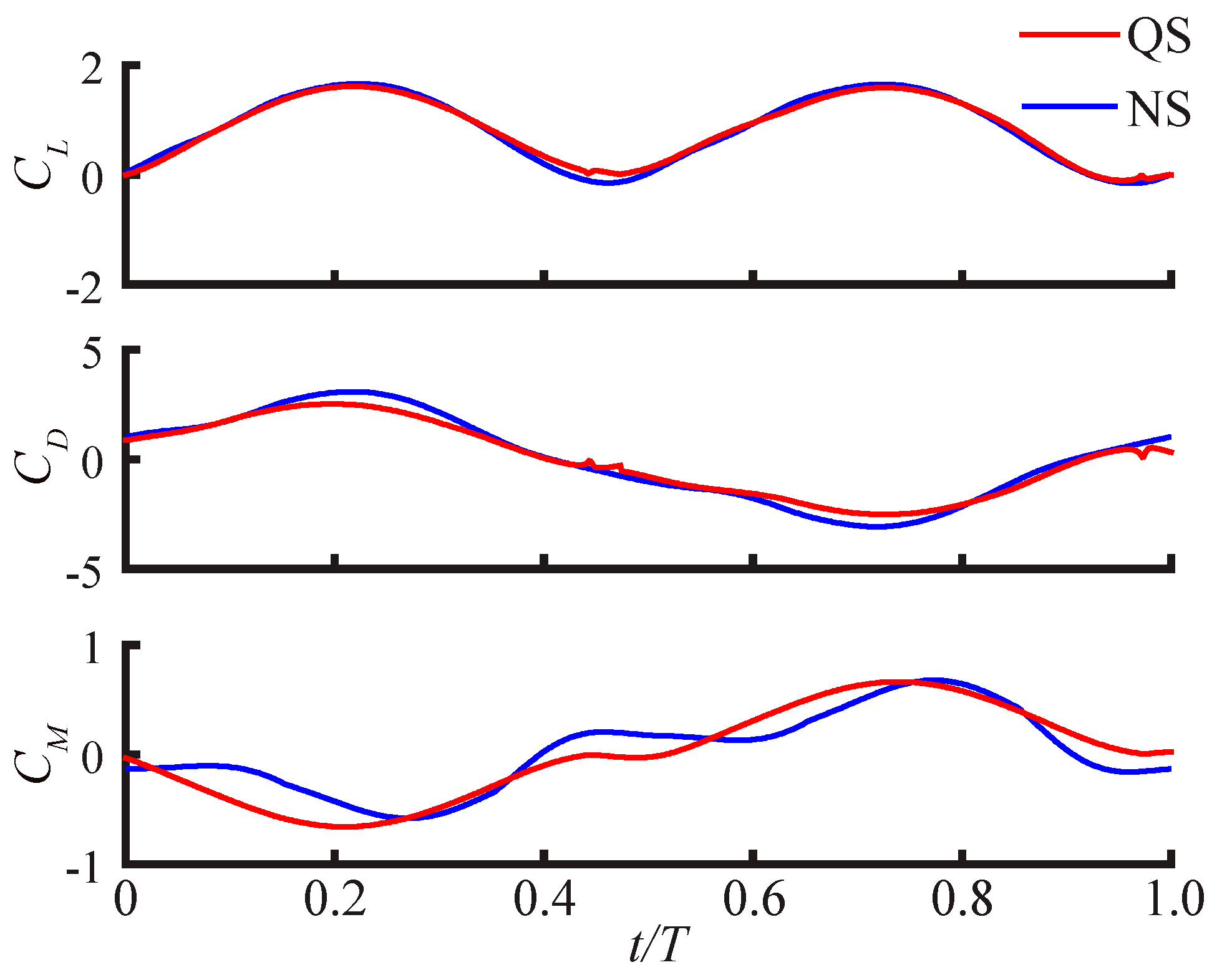
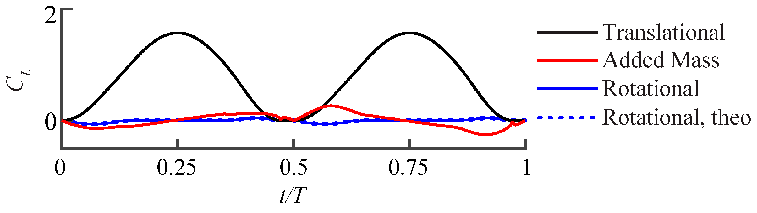
3.2.2. Smallest Difference Motion: Case 22

While the largest difference in accuracy between the models is seen when the pitching kinematics are extreme, the smallest differences are seen when the kinematics are mild. Consider as an illustrative example the motion with x_pa = 0.5, A = 30°, and Δτ_r = 0.3. This motion shows a difference in the cycle-averaged lift of only 0.01 between QS and NSe.

We plot the direct comparison of lift, drag, and moment coefficient for this motion in Figure 16. Compared to the large difference case, the magnitude of the coefficients is smaller in general. Because the duration of the pitching motion is long at Δτ_r = 0.3, the wing does not pitch as quickly. This motion is directly seen in the QS lift coefficient which is mostly sinusoidal. The QS shows a peak at the middle of the forward stroke and low values at stroke transition. The NSe model also predicts lowest values at the stroke transitions. However, the lift and drag time histories consist of multiple peaks. The first peak in the NSe lift is associated with wake capture, which a QS model cannot capture, and the second with the delayed stall due to the LEVs [40].

Figure 17 shows the breakdown for the QS components of lift. The translational component is the largest contributor to lift with only small effects from the added mass and rotational components during pitching. The translational lift is dominant due to the small pitching amplitude and the pitching axis being located at the mid-chord, resulting in in the pitching motion being less extreme and lasting longer over the stroke.

At the beginning of the forward stroke between t/T = 0.0 and t/T = 0.15, the wing begins to flap and to pitch down. The pitching amplitude is relatively small, i.e., A = 30°. Also, the pitching axis at the mid-chord, leading to a small rotational and added mass components. The added mass and rotational components are proportional to the pitching velocities and accelerations respectively. During the midstroke, the wing has stopped pitching and is at the maximum pitching angle of 30°. The angle of attack is about AoA = 60°. The translational component of the lift is by far the dominant component of the lift. As shown in Figure 11a, a previously shed vortex interacts with the wing, momentarily enhancing the lift. This wake-capture is reflected in the lift as a small peak at t/T = 0.1. The QS model is unable to capture this unsteady phenomenon. As the wing flaps further, a LEV forms on the top side of the wing, leading to delayed stall and increased lift. The NSe model matches very closely with the QS, suggesting that the translational component of the QS accurately models the delayed stall effect for this motion. At the end of the stroke, the pitching begins to take the wing back from the maximum angle of attack to 90°. The NSe lift is larger than the QS lift. The difference may again be ascribed by the inaccuracy of the rotational force term in the QS model. Similar trends are observed for the drag and moment about the pitch axis.

Figure 17 also indicates that the theoretical rotational force magnitude and the rotational force based on the empirical fit are nearly the same. This is a coincidence due to the fact that C_rot,exp = 3.14, which is close to the theoretical value of C_rot,theo = π [18]. It should also be noted that the added mass contribution in both Figure 13 and Figure 16 are not symmetric between the upstroke and downstroke. It is, however, expected that the added mass contribution would be symmetric between the two strokes when symmetric kinematics are implemented. It appears that this asymmetry is a result of the QS model’s formulation of the added mass force (Equation (7)) which is dependent on the sign convention used in defining the wing motion. This is demonstrated by Sane and Dickinson’s plots of lift due to added mass, which show slight asymmetries as well [18].

4. Concluding Remarks

The main purpose of this study is to quantify the differences and accuracy between two flapping wing aerodynamic models: (i) the quasi-steady model and (ii) 3D Navier–Stokes solutions for flapping wing flyers. When the pitching motion is extreme, i.e., the pitching motion is large, quick, and occurs about the leading or trailing edge, large force and moment magnitudes are seen at the beginning and end of the strokes. The differences between the QS and NSe are relatively also larger. The main difference is caused partially by the inaccuracy of the rotational lift term in the QS model, which is the dominant term at the beginning and end of the strokes. The use of theoretical value for the rotational coefficient worsens the accuracy of the force predictions compared to the use of empirically fit coefficient. Because the rotational effects are more important for the extreme pitch motions, the error caused by the rotational lift term is also more pronounced.

On the other hand, for the mild pitching motions with pitching motion that is small, long, and occurs about midchord, the translational contributions are more dominant. The translational term in the QS model provides a relatively accurate prediction. Another source for the difference is the inability of the QS model to properly capture the wake-capture, which is a nonlinear wing-wake interaction flow phenomenon.

This study is of particular importance to the modeling and analysis of the flight dynamics of bio-inspired MAVs or biological flyers. Due to the inherent coupling between the unsteady aerodynamics of the wings and flight dynamics of the body, a closed form expression, such as a QS model, would be used for the flapping aerodynamics in an ideal case as solving the NSe is computationally expensive. However, our study shows that the large and rapid pitch rotations that produce large forces, desired for MAV development, the current QS model underperforms. A question still remains how the observed differences in the aerodynamics would affect the MAV dynamics and stability, which will be investigated in the future.

Finally, Lentink and Dickinson [42] have shown that aerodynamic coefficients are sensitive to the Reynolds number especially Re < 1000, which is relevant to small insect and micro-air vehicles. The accuracy of QS model needs to be investigated at different Re. Also, as most insect wings are flexible, an investigation into the QS model performance as compared to flexible NSe models would be beneficial. Furthermore, this study only considered three pitching parameters, leaving numerous kinematic parameters left as unexplored topics of future studies. Another avenue for future research would be to investigate additional QS models [8,17,18,19,20,21,22,23,24,25,26,27] and compare them against each other as well as against Navier–Stokes solvers.

References

1. Salmon, J.L.; Bluman, J.E.; Kang, C.-K. Quasi-steady versus Navier-Stokes Solutions of Flapping Wing Aerodynamics. In Proceedings of the 55th AIAA Aerospace Sciences Meeting, Grapevine, TX, USA, 9–13 January 2017; pp. 1–21. [Google Scholar] [CrossRef]
2. Ma, K.Y.; Chirarattananon, P.; Fuller, S.B.; Wood, R.J. Controlled Flight of a Biologically Inspired, Insect-Scale Robot. Science 2013, 340, 603–607. [Google Scholar] [CrossRef] [PubMed]
3. Shyy, W.; Aono, H.; Chimakurthi, S.K.; Trizila, P.; Kang, C.; Cesnik, C.E.S.; Liu, H. Recent Progress in Flapping Wing Aerodynamics and Aeroelasticity. Prog. Aerosp. Sci. 2010, 46, 284–327. [Google Scholar] [CrossRef]
4. Shyy, W.; Aono, H.; Kang, C.-K.; Liu, H. An Introduction to Flapping Wing Aerodynamics; Cambridge University Press: New York, NY, USA, 2013; ISBN 9781107037267. [Google Scholar]
5. Shyy, W.; Kang, C.K.; Chirarattananon, P.; Ravi, S.; Liu, H. Aerodynamics, sensing and control of insect-scale flapping-wing flight. Proc. R. Soc. A Math. Phys. Eng. Sci. 2016, 472, 20150712. [Google Scholar] [CrossRef] [PubMed] [Green Version]
6. Weis-fogh, T. Quick estimates of flight fitness in hovering animals, including novel mechanisms for lift production. J. Exp. Biol. 1973, 59, 169–230. [Google Scholar]
7. Bergou, A.J.; Xu, S.; Wang, Z.J. Passive wing pitch reversal in insect flight. J. Fluid Mech. 2007, 591, 321–337. [Google Scholar] [CrossRef]
8. Dickinson, M.H. Wing rotation and the aerodynamic basis of insect flight. Science. 1999, 284, 1954–1960. [Google Scholar] [CrossRef] [PubMed]
9. Weis-Fogh, T. Energetics of Flight in Hummingbirds and in Drosophila. J. Exp. Biol. 1972, 56, 79–104. [Google Scholar]
10. Wang, Z.J. Dissecting Insect Flight. Annu. Rev. Fluid Mech. 2005, 37, 183–210. [Google Scholar] [CrossRef]
11. Sun, M.; Xiong, Y. Dynamic flight stability of a hovering bumblebee. J. Exp. Biol. 2005, 208, 447–459. [Google Scholar] [CrossRef] [PubMed] [Green Version]
12. Sun, M.; Tang, J. Unsteady aerodynamic force generation by a model fruit fly wing in flapping motion. J. Exp. Biol. 2002, 205, 55–70. [Google Scholar] [PubMed]
13. Sane, S.P. The aerodynamics of insect flight. J. Exp. Biol. 2003, 206, 4191–4208. [Google Scholar] [CrossRef] [PubMed] [Green Version]
14. Ellington, C.P. The Aerodynamics of Hovering Insect Flight. I. The Quasi-Steady Analysis. Philos. Trans. R. Soc. B Biol. Sci. 1984, 305, 1–15. [Google Scholar] [CrossRef]
15. Ellington, C.P. The Aerodynamics of Hovering Insect Flight. II. Morphological Parameters. Philos. Trans. R. Soc. Lond. Ser. B-Biol. Sci. 1984, 305, 17–40. [Google Scholar] [CrossRef]
16. Ellington, C.P. The Aerodynamics of Hovering Insect Flight. III. Kinematics. Philos. Trans. R. Soc. B Biol. Sci. 1984, 305, 41–78. [Google Scholar] [CrossRef]
17. Andersen, A.; Pesavento, U.; Wang, Z.J. Unsteady aerodynamics of fluttering and tumbling plates. J. Fluid Mech. 2005, 541, 65–90. [Google Scholar] [CrossRef]
18. Sane, S.P.; Dickinson, M.H. The aerodynamic effects of wing rotation and a revised quasi-steady model of flapping flight. J. Exp. Biol. 2002, 205, 1087–1096. [Google Scholar] [PubMed]
19. Berman, G.J.; Wang, Z.J. Energy-minimizing kinematics in hovering insect flight. J. Fluid Mech. 2007, 582, 153–168. [Google Scholar] [CrossRef]
20. Bolender, M.A. Open-Loop Stability of Flapping Flight in Hover. In Proceedings of the AIAA Guidance Navigation Control Conference Exhibition, Toronto, ON, Canada, 2–5 August 2010; pp. 1–18. [Google Scholar] [CrossRef]
21. Dickson, W.B.; Straw, A.D.; Dickinson, M.H. Integrative Model of Drosophila Flight. AIAA J. 2008, 46, 2150–2164. [Google Scholar] [CrossRef] [Green Version]
22. Wang, Z.J.; Birch, J.M.; Dickinson, M.H. Unsteady forces and flows in low Reynolds number hovering flight: Two-dimensional computations vs robotic wing experiments. J. Exp. Biol. 2004, 207, 449–460. [Google Scholar] [CrossRef] [PubMed]
23. Han, J.-S.; Chang, J.W.; Cho, H.-K. Vortices behavior depending on the aspect ratio of an insect-like flapping wing in hover. Exp. Fluids 2015, 56, 181. [Google Scholar] [CrossRef]
24. Hedrick, T.L.; Daniel, T.L. Flight control in the hawkmoth Manduca sexta: The inverse problem of hovering. J. Exp. Biol. 2006, 209, 3114–3130. [Google Scholar] [CrossRef] [PubMed]
25. Khan, Z.A.; Agrawal, S.K. Optimal Hovering Kinematics of Flapping Wings for Micro Air Vehicles. AIAA J. 2011, 49, 257–268. [Google Scholar] [CrossRef]
26. Sane, S.P.; Dickinson, M.H. The control of flight force by a flapping wing: Lift and drag production. J. Exp. Biol. 2001, 204, 2607–2626. [Google Scholar] [PubMed]
27. Lee, Y.J.; Lua, K.B.; Lim, T.T.; Yeo, K.S. A quasi-steady aerodynamic model for flapping flight with improved adaptability. Bioinspir. Biomim. 2016, 11, 036005. [Google Scholar] [CrossRef] [PubMed]
28. Nakata, T.; Liu, H.; Bomphrey, R.J. A CFD-informed quasi-steady model of flapping-wing aerodynamics. J. Fluid Mech. 2015, 783, 323–343. [Google Scholar] [CrossRef] [PubMed] [Green Version]
29. Taha, H.E.; Hajj, M.R.; Nayfeh, A.H. Flight dynamics and control of flapping-wing MAVs: A review. Nonlinear Dyn. 2012, 70, 907–939. [Google Scholar] [CrossRef]
30. Bluman, J.E.; Kang, C.-K. Wing-wake interaction destabilizes hover equilibrium of a flapping insect-scale wing. Bioinspir. Biomim. 2017, 12, 046004. [Google Scholar] [CrossRef] [PubMed]
31. Lua, K.B.; Lim, T.T.; Yeo, K.S. Scaling of aerodynamic forces of three-dimensional flapping wings. AIAA J. 2014, 52, 1–7. [Google Scholar] [CrossRef]
32. Bluman, J.E.; Sridhar, M.K.; Kang, C. The Influence of Wing Flexibility on the Stability of a Biomimetic Flapping Wing Micro Air Vehicle in Hover. In Proceedings of the AIAA SciTech Forum: 57th AIAA/ASCE/AHS/ASC Structures, Structural Dynamics, and Materials Conference, San Diego, CA, USA, 4–8 January 2016. [Google Scholar]
33. Han, J.S.; Kim, J.K.; Chang, J.W.; Han, J.H. An improved quasi-steady aerodynamic model for insect wings that considers movement of the center of pressure. Bioinspir. Biomim. 2015, 10. [Google Scholar] [CrossRef] [PubMed]
34. Leishman, J. Principles of Helicopter Aerodynamics, 2nd ed.; Shyy, W., Rycroft, M.J., Eds.; Cambridge University Press: Cambridge, NY, USA, 2006; ISBN 0-521-85860-7. [Google Scholar]
35. Fung, Y.C. An Introduction to the Theory of Aeroelasticity; Dover Publications Inc.: Mineola, NY, USA, 2008. [Google Scholar]
36. Tang, J.; Viieru, D.; Shyy, W. Effects of Reynolds number and flapping kinematics on hovering aerodynamics. AIAA J. 2008, 46, 967–976. [Google Scholar] [CrossRef]
37. Shyy, W.; Lian, L.; Tang, J.; Liu, H.; Trizila, P.; Stanford, B.; Bernal, L.P.; Cesnik, C.E.S.; Friedmann, P.; Ifju, P. Computational aerodynamics of low Reynolds number plunging, pitching and flexible wings for MAV applications. Acta Mech. Sin. 2008, 24, 351–373. [Google Scholar] [CrossRef]
38. Lian, Y.; Shyy, W.; Viieru, D.; Zhang, B. Membrane wing aerodynamics for micro air vehicles. Prog. Aerosp. Sci. 2003, 39, 425–465. [Google Scholar] [CrossRef]
39. Kamakoti, R.; Shyy, W. Evaluation of geometric conservation law using pressure-based fluid solver and moving grid technique. Int. J. Heat Fluid Flow 2004, 14, 851–865. [Google Scholar] [CrossRef]
40. Trizila, P.; Kang, C.-K.; Aono, H.; Shyy, W.; Visbal, M. Low-Reynolds-number aerodynamics of a flapping rigid flat plate. AIAA J. 2011, 49, 806–823. [Google Scholar] [CrossRef]
41. Trizila, P.C. Aerodynamics of Low Reynolds Number Rigid Flapping Wing under Hover and Freestream Conditions; University of Michigan: Ann Arbor, MI, USA, 2011. [Google Scholar]
42. Lentink, D.; Dickinson, M.H. Rotational accelerations stabilize leading edge vortices on revolving fly wings. J. Exp. Biol. 2009, 212, 2705–2719. [Google Scholar] [CrossRef] [PubMed] [Green Version]
43. Fry, S.N.; Sayaman, R.; Dickinson, M.H. The aerodynamics of hovering flight in Drosophila. J. Exp. Biol. 2005, 208, 2303–2318. [Google Scholar] [CrossRef] [PubMed] [Green Version]
44. Aono, H.; Liang, F.; Liu, H. Near- and far-field aerodynamics in insect hovering flight: An integrated computational study. J. Exp. Biol. 2008, 211, 239–257. [Google Scholar] [CrossRef] [PubMed]
Figure 1. Schematic of the (a) wing geometry, (b) orthographic view of the flapping wing motion, (c) 2D view of the pitching motion for Δτr = 0.2, and (d) 3D design space with the design variables, pitch amplitude A, pitching duration Δτr and pitching axis location xpa along the chord.
Fluids 03 00081 g001
Figure 2. Images of (a) a fruit fly wing and (b) the corresponding 3D wing grid.
Fluids 03 00081 g002
Figure 3. Time history of the lift coefficient for the (a) spatial and (b) time sensitivity studies during the third flapping period. Note, all NSe results reported are from the third flapping period.
Fluids 03 00081 g003
Figure 4. NSe solutions of the cycle-averaged lift coefficient in the design space. (a) Iso-surfaces of <CL> in the design space. (b) Slices of <CL> in the design space at various xpa values.
Fluids 03 00081 g004
Figure 5. Plots of the predicted lift, drag, and moment coefficient for cases with changing pitching amplitude, A = 30° (black), A = 45° (red) and A = 60° (blue). (a) Mild motions with Δτr = 0.3 and xpa = 0.5; (b) Extreme motions with Δτr = 0.2 and xpa = 1.0.
Fluids 03 00081 g005
Figure 6. Contour plots of the NSe iso-surfaces of Q-criterion at Q = 0.75 for motions with Δτr = 0.3, xpa = 0.5 and (a) A = 30°, (b) A = 45°, and (c) A = 60°.
Fluids 03 00081 g006
Figure 7. Contour plots of the NSe coefficient of pressure on the top and bottom of the wing at the middle of the forward stroke (t/T = 0.25) for Δτr = 0.3 and xpa = 0.5; (a) A = 30°, (b) A = 45°, and (c) A = 60°.
Fluids 03 00081 g007
Figure 8. Plots of the predicted lift, drag, and moment coefficient for cases with changing pitching duration, Δτr = 0.2 (black), Δτr = 0.3 (red), and Δτr = 0.5 (blue). (a) Mild motion with A = 30° and xpa = 0.5; (b) Extreme motion with A = 60° and xpa = 1.0.
Fluids 03 00081 g008
Figure 9. Contour plots of the NSe iso-surfaces of Q-criterion at Q = 0.75 at t/T = 0.25 (top) and t/T = 0.5 (bottom) for motions with pitching duration, (a) Δτr = 0.2, (b) Δτr = 0.3, and (c) Δτr = 0.5; Mild motions with A = 30° and xpa = 0.5.
Fluids 03 00081 g009
Figure 10. Plots of the NSe predicted lift, drag, and moment coefficient for cases with changing pitching axis, xpa = 0.0 (black), xpa = 0.25 (red), xpa = 0.5 (blue), xpa = 0.75 (purple), and Δτr = 0.5 (green) (a) cases with A = 30° and Δτr = 0.3 (b) cases with A = 60° and Δτr = 0.2.
Fluids 03 00081 g010
Figure 11. NSe iso-surfaces of Q-criterion at Q = 0.75 and colored with Y- vorticity for the following motions: (a) xpa = 0, A = 30°, and Δτr = 0.3 at t/T = 0.0, (b) xpa = 0.5, A = 30°, and Δτr = 0.3 at t/T = 0.0, and (c) xpa = 1.0, A = 30°, and Δτr = 0.3 at t/T = 0.0.
Fluids 03 00081 g011
Figure 12. Contour plots of the differences in cycle-averaged lift coefficient between QS and NSe (<CL,QS> − <CL,NSe>) in the design space of the pitching axis (xpa), pitching duration (Δτr), and pitching amplitude (A). (a) Iso-surfaces of <CL,QS> − <CL,NSe> in the design space. (b) Slices of <CL,QS> − <CL,NSe> in the design space at various xpa.
Fluids 03 00081 g012
Figure 13. Plots of wing pitching and flapping for the smallest difference motion versus the largest difference motion. The largest difference motion is characterized by A = 60°, Z = 49.3°, Δτr = 0.2, and xpa = 1.0. The smallest difference motion is characterized by A = 30°, Z = 49.3°, Δτr = 0.3, and xpa = 0.5.
Fluids 03 00081 g013
Figure 14. Plots of coefficients of lift (top), drag (middle), and moment (bottom) over one stroke for QS (red) and NSe (blue) predictions for the largest difference motion. In the figure the cycle-averaged lift coefficient for the QS is 1.11 and the NSe is −0.59. A = 60°, Δτr = 0.2 and xpa = 1.0.
Fluids 03 00081 g014
Figure 15. Plots of the translational (black), added mass (red), rotational (blue) and theoretical rotational (blue dashed), added mass and rotational lift forces in the QS model for the largest difference motion. A = 60°, Δτr = 0.2, and xpa = 1.0.
Fluids 03 00081 g015
Figure 16. Plots of coefficients of lift (top), drag (middle), and moment (bottom) over one period for QS (red) and NSe (blue) predictions for the small difference motion. In the figure the cycle-averaged lift coefficient for the QS is 0.83 and the NSe is 0.82. A = 30°, Δτr = 0.3, and xpa = 0.5.
Fluids 03 00081 g016
Figure 17. Plots of the translational (black), added mass (red), rotational (blue) and theoretical rotational (blue dashed) lift forces in the QS model for the smallest difference motion. A = 30°, Δτr = 0.3, and xpa = 0.5.
Fluids 03 00081 g017