Predicting Energy Generation in Large Wind Farms: A Data-Driven Study with Open Data and Machine Learning

Abstract

Wind energy has become a trend in Brazil, particularly in the northeastern region of the country. Despite its advantages, wind power generation has been hindered by the high volatility of exogenous factors, such as weather, temperature, and air humidity, making long-term forecasting a highly challenging task. Another issue is the need for reliable solutions, especially for large-scale wind farms, as this involves integrating specific optimization tools and restricted-access datasets collected locally at the power plants. Therefore, in this paper, the problem of forecasting the energy generated at the Praia Formosa wind farm, an eco-friendly park located in the state of Ceará, Brazil, which produces around 7% of the state’s electricity, was addressed. To proceed with our data-driven analysis, publicly available data were collected from multiple Brazilian official sources, combining them into a unified database to perform exploratory data analysis and predictive modeling. Specifically, three machine-learning-based approaches were applied: Extreme Gradient Boosting, Random Forest, and Long Short-Term Memory Network, as well as feature-engineering strategies to enhance the precision of the machine intelligence models, including creating artificial features and tuning the hyperparameters. Our findings revealed that all implemented models successfully captured the energy-generation trends, patterns, and seasonality from the complex wind data. However, it was found that the LSTM-based model consistently outperformed the others, achieving a promising global MAPE of 4.55%, highlighting its accuracy in long-term wind energy forecasting. Temperature, relative humidity, and wind speed were identified as the key factors influencing electricity production, with peak generation typically occurring from August to November.

1. Introduction

Wind power is one of the fastest-growing forms of green energy production worldwide. According to the Global Wind Report (2023) [1], global wind power capacity grew by 9% in 2022 compared to 2021, adding 77.6 GW of fresh production while bringing the total installed capacity to 906 GW for the entire renewable energy industry. Unlike other conventional resources such as fossil fuel and even hydroelectric generation, the kinetic energy continually induced by circulating air is considered an inexhaustible source of power, which is abundant and widely distributed, making it a scalable source that can meet a variety of demands. Moreover, the adverse effects caused by wind plants do not drastically impact local fauna and flora, resulting in a clean and sustainable energy generation [2,3]. Another plus is that wind energy is economically competitive with other forms of generation, especially for countries and businesses seeking to reduce their carbon footprint and dependence on fossil fuels [4,5].

Despite the benefits and advances promoted by wind-driven generation, electricity produced in wind farms may undergo high volatility. For example, wind speed does not always follow a regular behavior over time. As a consequence, assessing and forecasting energy generation amid the incessant demand of consumption centers is not a straightforward task. In addition, the diversity of technologies and conversion systems used in wind turbines that coexist in large-scale power complexes contribute to generation volatility, thus imposing the necessity of using data-driven tools to keep power production constant, predictable, and reliable for dispatch and consumption. Another issue is that the weather conditions such as the airspeed, relative humidity, air temperature, atmospheric pressure, and precipitation can influence the trend and seasonality of the day-to-day-generated power, especially in large wind farms, resulting in irregular and highly non-linear data, which need to be handled when fitting machine learning models [6,7,8]. Lastly, the electricity load from wind power plants can affect the law of supply and demand in the energy wholesale market [9], rendering data-driven learning approaches crucial for gaining more-assertive insights for decision-making in this business sector.

In general, the problem of assessing and forecasting the power generation in large wind farms involves investigating the trend and seasonality of combined time series data. According to Quian and Sui [10], renewable energy prediction planning horizons can be categorized into three groups: (i) short-term (one hour to seven days), (ii) medium-term (one week to one month), and (iii) long-term (one month to one year). Long-term forecasting is crucial for achieving grid balance, infrastructure construction and maintenance, as well as strategic energy planning [10]. Since the prediction is usually computed by assuming a specific forecast horizon, the long-term case is more challenging due to the high variability of wind power over an extended period, making the forecast task by machine learning models difficult in real-world scenarios [11,12,13].

In the specialized literature, various machine-learning-based approaches have been proposed to estimate energy generation in wind farms. For example, Zheng et al. [7] employed a Feature Selection Engineering (FSE) step using k-means clustering to build a learning methodology based on the XGBoosting (XGB) algorithm for short-term power forecasting. To train their model, the authors took weather-type features such as temperature, air humidity, and precipitation data. Paula et al. [12] also applied FSE to improve the discriminative performance of machine learning methods, including Artificial Neural Networks (ANNs), Random Forest (RF), and Gradient Boosting (GB), to estimate wind-related features, while Demolli et al. [8] utilized XGB, RF, Support Vector Machine (SVM), and Lasso Regression (LG) to compute daily power predictions by inputting wind speed data. Along the same line, Singh et al. [14] employed a GB-based regression approach to explore the problem of power generation forecasting in Turkish wind farms, delivering short-term predictions. Wind power forecasting was also the goal of Optis and Perr-Sauer [15], where the stability of the machine learning algorithms Multilayer Perceptron (MLP), Extremely Randomized Trees (ERT), GB, and SVM was assessed by considering the effect of atmospheric turbulence during the problem modeling. Similarly, Li et al. [16] took the SVM algorithm together with a recent swarm-based optimization method called dragonfly to predict wind power over a short-term period.

The combination of machine learning and statistical analysis is another effective approach that offers an in-depth examination of wind farm data, including forecasts. In this domain, Malska and Damian [17] conducted an immersive statistical analysis of energy production in a wind farm located in the Subcarpathian region, Poland. Adopting a similar methodology, Shabbir et al. [18] implemented a recurrent neural network architecture combined with advanced statistical methods to estimate energy generation in an Estonian wind farm. Najeebullah et al. [19] also applied a statistical framework for wind power prediction, obtaining short-term forecasts through a hybrid modeling based on ANN models. Puri and Nikhil [20] investigated the availability of wind energy in highly mountainous regions, specifically in the Himalayan Range. Their study employed data on wind speed, temperature, and air density to predict wind energy using ANN-based algorithms, with the goal of enhancing future planning for wind electricity production. Solari et al. [21] covered forecast horizons restricted to a few days by taking geostrophic wind data to infer wind speed for port safety purposes. In a similar way, Cheng et al. [22] aimed at achieving short-term outputs by predicting wind-related features based on anemometer data.

Finally, Long Short-Term Memory (LSTM) networks have recently been used to tackle time series prediction applications. In this context, Vaitheeswaran and Ventrapragada [23] employed a hybrid approach integrating LSTM and Genetic Algorithms (GAs) for wind power prediction, aiming to achieve both short-term and medium-term forecasts. Jaseena and Kovoor [24] demonstrated that their LSTM-based method outperforms the classic ARIMA technique in short-term wind speed forecasting. Sowmya et al. [25] also addressed the wind forecasting problem, by applying stacked LSTM architectures instead. Papazek and Schicker [26] explored different application scenarios by integrating time series data from diverse sources using LSTM, underscoring the importance of customized pre- and post-processing methods in renewable energy prediction. Ziaei and Goudarzi [27] developed LSTM-driven models specifically for short-term wind estimation, showcasing their effectiveness in capturing wind characteristics with satisfactory accuracy. In a similar fashion, Kumar et al. [28] applied LSTM and Recurrent Neural Networks (RNNs) for predicting wind speed and solar irradiance. The forecasted renewable energy data were then utilized to analyze the load frequency behavior in an isolated microgrid.

As pointed out by Wilczak et al. [29] and Mesa et al. [30], wind power estimation has always been of interest to the energy community; however, the main focus has been on improving short-term wind forecasts instead. Moreover, according to Wang et al. [31], most regular- and long-term wind power forecasts are primarily designed for individual sites and suffer from certain shortcomings, such as ignoring regional characteristics. Another concern related to extended-range forecasts is that obtaining a computationally robust solution for large-scale wind farms in practice may require the unification of customized tuning approaches, sophisticated optimization models, and accurate machine learning models, as well as the availability of extensive, restricted-access datasets locally acquired from the power plants [13,32]. These datasets include not only energy-related data collected from the wind farms, but also the systematic assessment of local meteorological variables.

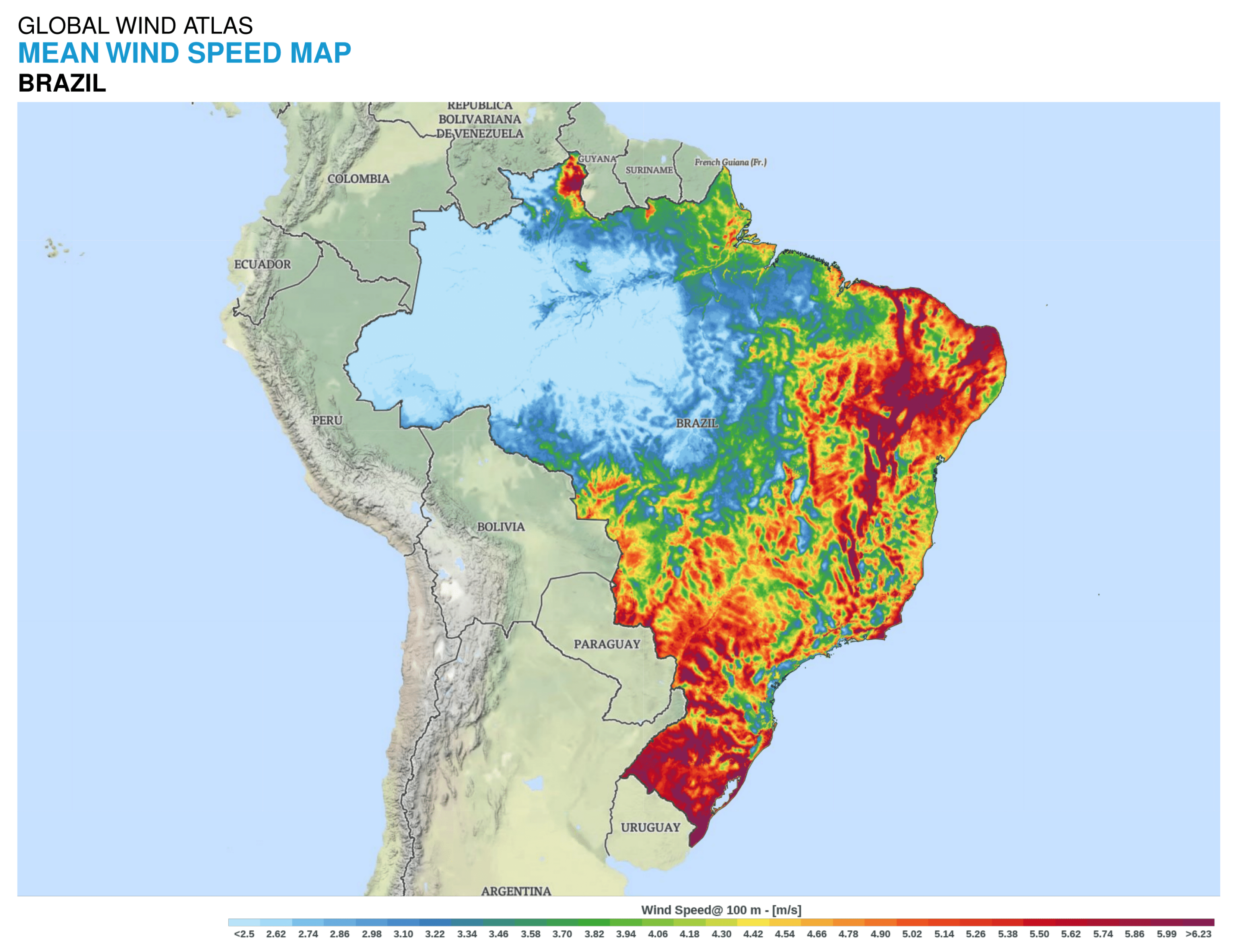
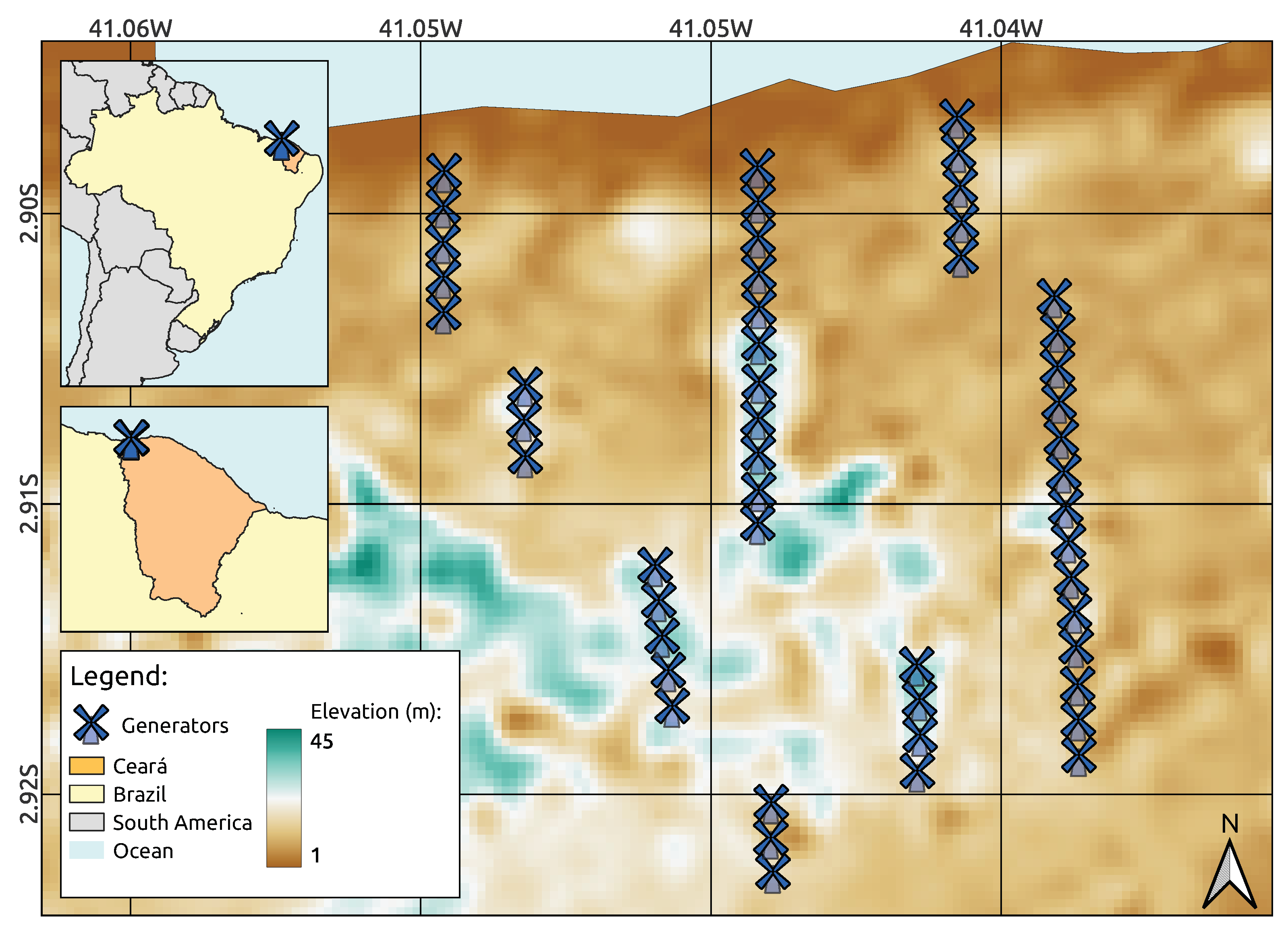
Therefore, in this paper, the focus was on providing an effective data-driven methodology for assessing and predicting the electricity generated at one of the largest renewable energy farms in South America: the Praia Formosa wind complex, located in the municipality of Camocin, in the state of Ceará, Brazil, with an installed capacity of 104.4 MW. To tackle most of the issues raised above, an integrated database was built using open data repositories to train three machine intelligence models: Random Forest, Extreme Gradient Boosting, and Long Short-Term Memory Network, enabling accurate and consistent long-term forecasts. Specifically, public data from both regional weather stations and the National Electric Systems Operator were collected in an effort to improve the model’s predictability by exploiting external factors that may influence wind power generation in this region. As a result, the formulated holistic framework not only enhanced the forecasting accuracy, but also provided valuable insights into the interplay between regional weather conditions and local energy production throughout different periods of the year. Additionally, data-driven strategies, including the use of feature engineering tools, were employed to optimize the accuracy of the machine intelligence models while evaluating the influence of meteorological variables on wind farm power generation.

In summary, the key contributions of this paper are:

• The design of three accurate, well-behaved machine learning approaches for long-term forecasting: the RF-, XGB-, and LSTM-based models. Unlike most predictive proposals in the wind energy context, which focus on short-term results, the designed models excel in delivering precise long-range wind power outputs.
• The creation of a comprehensive database sourced from multiple open platforms, enabling a thorough analysis of the regional characteristics of the wind farm.
• The implementation of customized tuning strategies to optimize the machine intelligence models, leading to significant improvements in long-range predictions.
• An in-depth data-driven study of key meteorological variables that most influence wind power generation throughout different seasons and months, providing detailed insights and contextualization for local grid operators and power plant owners.

2. Materials and Methods

2.1. Study Area

As our study area, the Praia Formosa wind complex was chosen due to its status as having one of the largest installed capacities in Brazil [33]. Initiating its operations on 26 August 2009, the Praia Formosa wind park comprises 50 Suzlon S-88 wind turbines, collectively generating a total capacity of 104.4 MW [34]. This power complex is situated in Camocim, a picturesque coastal town situated in the state of Ceará, Brazil, that offers an ideal setting for wind energy generation. Influenced by strong ocean-derived currents, this east coastal region experiences an annual average wind speed ranging between 7 and 10 m/s [35]. Moreover, wind speed intensifies during the second half of the year, especially due to the phenomenon of the maximum high-pressure center in the South Atlantic basin, known as the South Atlantic Anticyclone (SAA) [36]. The Brazilian Northeast region accounts for 86% of the total wind energy generated in the country [37]. The average wind distribution across Brazil, as measured and mapped by the Global Wind Atlas, is illustrated in Figure 1.

Conducting data-driven investigations on well-established large-scale power plants, such as the one selected for this study, aims to gather findings, insights, and technical data to support the expansion of renewable sources in Brazil. This includes providing data-driven assistance for both wind farms under construction and those already announced, thus advancing sustainable energy solutions in this key region. The location of the studied wind farm in the Brazilian northeast is shown in Figure 2.

2.2. Data Repositories

In order to build a representative database for investigating and predicting wind generation at the Praia Formosa wind complex, open data from multiple Brazilian government agencies were taken. In particular, both energy-related and meteorological datasets were collected from the following public repositories: (i) the National Electric Systems Operator (ONS—acronym in Portuguese) [39], which is the core body responsible for coordinating and controlling the energy generation and transmission in Brazil, and (ii) the National Institute of Meteorology (INMET—acronym in Portuguese) [40], which is the agency that measures and monitors the country’s weather conditions in all Brazilian localities.

The ONS provides wind energy generation data and other power-related features of wind farms in Brazil, including the Praia Formosa one. The raw data can be collected as time series and arranged into specific time horizons such as hourly, daily, monthly, or annually. In our approach, time series comprising daily instances of wind energy-related data were taken as input. The data collected spans from 1 January 2016, to 31 December 2022, a full seven-year period totaling 2.557 data samples (see Supplementary Materials). Meteorological data were also gathered on a daily basis from the Sobral’s city weather station, which is located in the Praia Formosa wind farm region. For better readability of the acquired data,

Table 1. Main set of collected data, arranged on a daily basis.

Feature	Description	Unity	Repository
Date	Day, month, year and season	-	-
Temperature	Average temperature	${}^{\circ }$C	INMET
Relative humidity	Average relative humidity	%	INMET
Pressure	Average pressure	hPa	INMET
Precipitation	Average precipitation rate	mm/d	INMET
Wind speed	Average wind speed	m/s	INMET
Max energy demand	Wind energy load demand peak	MWmed	ONS
Wind energy generation	Total generated by the power plants	MWmed	ONS

summarizes the main features used to drive our data analysis and machine learning predictions.

2.3. Machine Learning Algorithms for Wind Energy Prediction

In this section, the theoretical aspects of the three machine learning methods used in our wind power prediction assessments, namely RF, XGB, and LSTM, are provided. The selection of these methods was shaped by [8,41], where the authors emphasized the effectiveness of RF, XGB, and LSTM in accurately forecasting long-term wind power when compared to other long-horizon algorithms.

2.3.1. Extreme Gradient Boosting-Based Model

The Extreme Gradient Boosting (XGBoosting or XGB) method is a tree-based machine learning approach that aims to enhance gradient boosting while handling various differentiable loss functions [42].

Similar to the well-established Gradient Boosting (GB) method [43], the XGBoosting technique adopts weak learners through the application of the gradient descent method. However, XGB improves the GB architecture in terms of regularization and gradient approximation, as well as effectively handling missing values, ensuring high customizability. Technically, the weights taken in the decision trees are non-uniform, which reduces overfitting in the trained model.

To leverage the varying weights while training the XGB model, the algorithm minimizes the following loss function:

$$L_t=\sum _{}^{}l(y_i{\widehat{y}}_i^{(t-1)}+f_t\left(x_i\right))+\Omega \left(f_t\right),$$

(1)

where $y_i$ is the target feature, ${\widehat{y}}_i^{(t-1)}$ is the predicted value at $t-1$ time, $f_t\left(x_i\right)$ is the prediction of tree t on the training sample i, and $\Omega \left(f_t\right)$ is the regularization term used to prevent overfitting. The goal of XGB is to minimize Equation (1) to determine the optimal parameters of the model, which are the set of trees $f_t$ that collectively contribute to decreasing the loss function. Another advantage offered by the XGB-based learning process is the incorporation of regularization terms such as $reg\_lambda$ and $reg\_alpha$ [44]. These terms assign varying weights to the leave nodes, allowing the model to remove or split trees of small importance during the training stage, thus improving overall performance [44].

Computationally, the algorithm involves the choice of the following parameters during its implementation:

• The cost function, Equation (1), to be optimized.
• The predictive models, which are defined as decision trees.
• Weak learners, to improve the minimization of the cost function.
• Regularization terms.

Notice that the configurations and the selection of the model’s hyperparameters will be discussed in the implementation section.

2.3.2. Random Forest-Based Model

The Random Forest (RF) algorithm is a robust and highly successful machine learning approach that produces predictions from a set of estimators. It takes into account both learning and modeling strategies based on regression or classification trees [45]. The RF algorithm relies on the principle of constructing a random subset during the nodes’ selection. As a result, the randomization allows the inclusion of variables that most influence the model, regardless of correlation, thereby substantially improving the algorithm’s performance [46].

In summary, the Random Forest method consists of applying the following steps:

• Generate X sets of bootstrap samples for the training dataset.
• For each sample, build a regression tree (without adjustment) with the following modification: at each node, generate a random sample P of the input variables from the training dataset and choose the best split of these, where $P<V$, and V is the number of variables in the dataset.
• Predict the new output, from averaging the outputs of M regression trees when new variables are inserted into the model.

2.3.3. Long Short-Term Memory-Based Model

Long Short-Term Memory (LSTM) networks are very effective, memory-enhanced neural architectures designed for modeling and learning complex temporal patterns in sequential data. In particular, LSTM-based models rely on a sophisticated neuro-mathematical paradigm, employing a recurrent neural structure that captures and retains information over extended time intervals. In contrast to classical artificial neural networks, LSTM-inspired approaches are purpose-built for coping with time-varying samples, learning long-term dependencies among data [47].

Mathematically, a prototype of the LSTM-type network can be described by the following equations:

$$f_t=\sigma (W_f·[h_{t-1},x_t]+b_f)$$

(2)

$$i_t=\sigma (W_i·[h_{t-1},x_t]+b_i)$$

(3)

$$o_t=\sigma (W_o·[h_{t-1},x_t]+b_o)$$

(4)

$$\tilde{c}t=tanh(W_c·[ht-1,x_t]+b_c)$$

(5)

$$c_t=f_t\odot c_{t-1}+i_t\odot {\tilde{c}}_t$$

(6)

$$h_t=o_t\odot tanh\left(c_t\right)$$

(7)

In Equations (2)–(7), $x_t$ represents the input at time t, $h_{t-1}$ is the previous hidden state, $\sigma$ is the activation function, ⊙ denotes element-wise multiplication, and the set $\{W_f,W_i,W_o,W_c,b_f,b_i,b_o,b_c\}$ gathers the parameters of the network [48]. In short, Equations (2)–(7) describe the process of updating the memory cell ($c_t$) and the hidden state ($h_t$) at each time step, making LSTM networks effective at capturing temporal patterns in sequential data.

In this study, a novel methodology tailored to the specific challenges posed by power prediction at the Praia Formosa wind complex was designed. Leveraging the rich dataset provided by the ONS, the Brazilian energy agency, our LSTM-based approach combines the power of recurrent neural network models with meteorological data to create a robust forecasting framework. Moreover, the trained model is capable of capturing both short-term fluctuations and long-term trends in energy generation, which is crucial for accurate forecasting.

2.4. Data Preparation and Standardization

To construct our machine intelligence models for the forecasting task, the acquired data was divided into training and testing subsets. More specifically, approximately 86% of the collected data (daily records ranging from 1 January 2016, to 31 December 2021, totaling 2192 instances) were used to train the models, while the remaining 14% of the data, covering the 365 days of 2022, were employed for long-term prediction validation. Prior research has indicated that a one-year time frame is considered a suitable choice when performing long-term predictions in the renewable energy context. Particularly, such a forecasting horizon is crucial for grid planning, scheduling, understanding seasonal effects, and ensuring the availability of valid data, as discussed in [10,49,50]. All features were scaled to a common range of $[0,1]$ to mitigate the impact of different units and scales between variables, thus reducing the scalability bias imposed by the collected data.

The machine learning models, as well as the KDD analysis codes related to the results exploded in Section 3.1 were implemented using the routines and functions available in the Scikit-learn library [51], a robust and well-established Python implementation tool.

2.5. Evaluation Metrics

In this section, the evaluation metrics used to quantitatively assess the predictive performance of our machine learning models are introduced. These include as validation metrics the Mean Absolute Percentage Error (MAPE) [52,53], the Mean Squared Error (MSE) [12], and the Mean Absolute Error (MAE) [11,12], which are mathematically computed by Equations (8)–(10):

$$MAPE=\frac{1}{n}\sum _{i=1}^n\left|\frac{Y_i-{\widehat{Y}}_i}{Y_i}\right|\times 100,$$

(8)

$$MSE=\sum _{i=1}^n{(Y_i-{\widehat{Y}}_i)}^2,$$

(9)

$$MAE=\frac{1}{n}\sum _{i=1}^n\left|Y_i-{\widehat{Y}}_i\right|,$$

(10)

where $Y_i$ and ${\widehat{Y}}_i$ denote the actual and predicted values for the target variable, respectively. In our validation results, a threshold of 10% was defined for MAPE [11,54], establishing a “high level” of predictive accuracy for the outputs.

2.6. Model’s Design, Implementation Schemes, and Tuning Strategies

In this section, the modeling steps to generate our machine learning models are given. Moreover, the strategies used for tuning the hyperparameters of these models are outlined, ensuring they are finely calibrated for optimal predictive performance.

2.6.1. Artificially Created Features

In order to computationally improve the performance of the machine learning models, a set of artificial features was created by systematically performing potential combinations among the ordinary variables and by conducting Knowledge Data Discovery (KDD Analysis), as discussed in Section 3.1. After a thorough data-driven investigation, seven new features were selected:

• Log return (Z) in the daily horizon, computed as follows: $Z_i=log(X_i/X_{i-1})$, $i=2,3,\dots ,n$, where $X_i$ accounts for the $i-th$ value of the wind power and n is the total number of instances. For more details, see [11,55].
• Moving average ($MA$) in the weekly, monthly and quarterly horizons. In more mathematical terms: $M{A}_i=\frac{1}{p}{\sum }_{j=1}^p{X}_{i-j-1}$, where p stands for the given horizon. For more details, see [11,56].
• Sum (S) of temperature (T) and humidity (H): $S_i=T_i+H_i$.;
• Subtraction (D) of temperature and humidity: $D_i=T_i-H_i$;
• Division (Q) of temperature by wind speed (W): $Q_i=T_i/W_i$;
• Moving subtraction ($MS$) of wind power: $M{S}_i=X_i-X_{i-1}$;
• Moving subtraction of temperature.

Additionally, from the daily energy generation data as analyzed in the KDD step, a cyclical feature capturing the generation trends throughout the weeks and a categorical attribute computed via the One-Hot encoding technique [57] to cover categorical data as a binary representation were introduced. Specifically, twelve binary variables were created, one for each month, to indicate whether a data point belongs to that month or not. These variables act as indicators, enabling the machine learning models to recognize the presence or absence of each month in the data. Moreover, they allow the models to consider seasonality and monthly patterns in energy generation, which are critical features for accurate forecasting and understanding how different months influence wind energy production.

After generating the set of newly crafted features, attribute selection was performed using a forest of trees, i.e., by employing a Random-Forest-based classifier to compute the impact of the features as part of the forecasting task. The Random Forest algorithm determines the feature importance through the application of the Gini Index, which can be formulated in its binary classification form as follows [58]:

$$Gini=p_1(1-p_1)+p_2(1-p_2),$$

(11)

where $p_1$ and $p_2$ are the probabilities of classes 1 and 2. Features that result in substantial reductions in the Gini Index are deemed more important to the model because they significantly contribute to reducing impurity in the tree nodes and, consequently, to the accuracy of predictions [59].

The RF-based feature importance process was then applied to identify the top 7 variables, as listed in Figure 3.

2.6.2. Machine Learning Hyperparameters’ Optimization

One of the main challenges when applying machine learning algorithms is to adequately calibrate their set of hyperparameters. These include the optimization of the learning rates, regularization coefficients, and the fine-tuning of feature engineering step, all of which significantly impact the model’s performance and generalization ability.

To tackle this issue, the Random Search (RS) method [60] was applied, which is an effective technique for hyperparameter tuning. RS efficiently explores the hyperparameter space, facilitating the discovery of optimal settings while enhancing the model’s overall effectiveness. Moreover, unlike other hyperparameter tuning techniques such as the well-known Grid Search, RS significantly reduces processing time by randomly sampling from a predefined set of values or features.

Table 2. Optimal hyperparameters and their search spaces for the XGBoosting model.

Hyperparameter	Description	Tuning Universe	Optimal Parameter
max_depth	Maximum tree depth	2, 3, 4, 5, 6, 7, 10	4
subsample	Subsample ratio of the training instances	0.1, 0.5, 0.7, 0.8, 0.9, 1	0.7
colsample_bytree	Subsample ratio of feature-like columns when constructing each tree	0.1, 0.4, 0.7, 0.8, 0.9, 1	1
n_estimators	Number of trees generated	25, 50, 100, 200, 300, 500	300
learning_rate	Learning rate of the model	0.01, 0.1, 0.2, 0.3	0.1

,

Table 3. Optimal hyperparameters and their search spaces for the Random Forest model.

Hyperparameter	Description	Tuning Universe	Optimal Parameter
n_estimators	Number of trees generated	25, 50, 100, 200, 500, 1K	50
max_depth	Maximum tree depth	2, 5, 10, 20, 30	20
min_samples_split	Minimum number of samples to split an internal node	2, 4, 6, 10	4
min_samples_leaf	Minimum number of samples for a leaf node	1, 2, 4, 6, 8	2
max_features	Maximum number of features for each split when constructing a decision tree	auto, sqrt, log2, none	log2

and

Table 4. Optimal hyperparameters and their search spaces for the LSTM model.

Hyperparameter	Description	Tuning Universe	Optimal Parameter
num_units_list	Number of units (or neurons) in the LSTM layer	32, 64, 128	64
activation	Activation function	identity, logistic, sigmoid, relu	sigmoid
solver	Mathematical solver for weight optimization	lbfgs, sgd, adam	adam
learning_rate_list	Manages weight update size during training	0.001, 0.01, 0.1	0.001
window_size_list	Number of past time steps LSTM considers for predicting the next step	5, 10, 15, 20	15

summarize the hyperparameter ranges found for each exploited machine learning model and the corresponding best set of values obtained.

3. Results

In this section, the quantitative analysis was conducted to explore the insights and findings from the Praia Formosa wind farm data, allowing for a deeper understanding of the energy generation trends while measuring the performance of our predictive models.

3.1. Knowledge Data Discovery

For a more comprehensive understanding of the Praia Formosa wind complex data, extensive Knowledge Data Discovery (KDD Analysis) was performed, including descriptive statistics, wind energy-related histograms and weekly/monthly boxplots concerning the full period of collected data, i.e., 1 January 2016, to 31 December 2022.

To address missing and erroneous data, the so-called missForest method [61] was taken, which trains the Random Forest algorithm on observed values within a data matrix to predict and impute the missing values [61]. Conceptually, the method builds an ensemble of decision trees to predict missing values based on the available information from other attributes within the dataset [62]. For a more comprehensive explanation of the missForest method, we refer to the seminal work by Stekhoven and Buhlmann [61].

First, measures of the central tendency for energy generation were computed so as to inspect its overall behavior. The measurements listed in

Table 5. Descriptive statistics analysis of the Praia Formosa’s Wind Farm.

Statistics	Wind Energy Generated (MWmed)
Average	23.98
Standard Deviation	15.27
25%	10.11
50%	23.85
75%	36.56

revealed that the power generation did not exhibit a normal distribution, as evidenced by the mean value exceeding the median (50%). This deviation from normality is further illustrated in Figure 4, which depicts the normalized distribution regarding the analyzed period (from 2016 to 2022). Furthermore, the plot highlights the presence of outliers that are skewed towards the higher end of the distribution. One can observe a few instances where the generation exceeds the baseline levels, centered around the mean and median over time.

Improving our understanding of how wind power generation correlates with factors such as wind speed and other meteorological variables is crucial for achieving more accurate predictions. In order to verify the linearity degree between the predictor variables and energy generation, in Figure 5, the Pearson correlation was computed. As observed in the heat bar plot, the target variable exhibits a strong negative correlation with relative humidity and a strong positive correlation with temperature and wind speed. These results are in line with the findings previously reported in the scientific literature. Particularly, according to [63], where the authors exploited over 40 papers on wind power forecasting, the most frequently used variables include wind speed, temperature, and relative humidity.

Figure 6 and Figure 7 display weekly and monthly boxplots of energy generation, allowing us to verify how wind energy varies over weeks and months, identifying patterns and potential outliers more clearly. By analyzing Figure 6, one can observe that the daily averages in the weekly boxplots remain consistent throughout the period of analysis.

In contrast, Figure 7 reveals that the average values in the monthly boxplots tend to be higher in the second half of the year, specifically from July to December, where a parabolic behavior of ascent and descent is observed. Furthermore, one can verify that there are a few outliers present in the distributions, especially during the months of June and July, coinciding with the onset of energy generation records.

The violin plot as displayed in Figure 8 presents the probability density of the electricity generated at the Praia Formosa wind complex (with a 95% confidence interval). From the plotted graph, it can be seen that there was a clear change in symmetry throughout the series. For instance, in March, a positive skewness was evident, indicating a clustering of values accumulated between 0 and 20 MWmed, while in the second semester, e.g., in October, the skewness reverses, with a concentration of values towards the higher end.

Finally, Figure 9 displays a facetgrid plot featuring density subplots organized by month. This plot effectively captures the nuances in the distributions of energy generation across the months of the year, revealing particular transitions and trends. January exhibits a wide dispersion of values between 0 and 40 MWmed, while from February to May, the values remain more consistent, mainly clustering in the range of 0 to 10. From June to August, there is a clear transition, with generation shifting from the 0–20 to 30–50 range. In contrast, the months of September to November are the ones that hold a high concentration of generation, with values predominantly above 40 MWmed, contrasting with December, which shows greater dispersion in generation.

3.2. Application of the Machine Learning Models for Wind Energy Forecasting

In this section, the focus is on the practical applications involving the implemented machine intelligence models supported by multiple data sources for the task of forecasting long-term predictions of energy generated at the Praia Formosa wind park.

In Figure 10, the evaluation metrics were computed for all the trained machine intelligent-based models as part of our quantitative analysis, where the optimized approaches were applied to predict the full period of testing, i.e., the whole year of 2022. By numerically inspecting the results delivered by the ensemble-built models XGB and RF, one can conclude that both approaches produced satisfactory results when evaluated via the MAPE and MSE metrics. Moreover, when considering only the MAPE evaluation metric, XGB reaches the 10% threshold of high accuracy, while RF slightly exceeded this baseline value by approximately 2%.

Despite the satisfactory results, a more accurate forecast was obtained by applying the LSTM-based framework. In fact, the trained recurrent neural network-based model was capable of effectively capturing the intricate temporal dependencies within the data, leading to high scores across all three evaluation metrics. For example, if one takes the MAPE as a baseline, the LSTM-based model achieved a surprising score of 4.55%, demonstrating robust consistency with the reference data. In general, good predictive performance was attained due to the combination of feature engineering step (including the creation of new features), hyperparameter optimization, and the strong correlations between predictor variables and the target one.

Figure 11 shows the forecasting plot of the wind energy generation for the last 30 days of 2022, as delivered by our tuned machine intelligence models, while Figure 12 displays the deviation (residue) between the actual and predicted values. Despite the usual high fluctuations in the actual energy generation time series, the forecasts closely mirror the real data in most of the instances, accurately capturing the cyclic patterns observed in the ground-truth curve, including the tendencies and the local extremes. This was more prominent for the trained LSTM-based model, which outperformed the others in terms of fitting capability and accuracy level, as evidenced by its residues being closer to zero.

In Figure 13, the evaluation metrics were listed for the same 30-day period as illustrated in Figure 11. Notably, when examining MSE, it is evident that LSTM achieved the lowest value at 1.59, indicating its superior ability to minimize prediction errors. In contrast, RF and XGB yielded higher MSE scores, suggesting relatively less precision in their forecasts. A similar trend persisted when considering the MAE and MAPE. However, it’s important to note that all three machine learning models achieved MAPE scores below 10%, indicating high accuracy in the prediction task. In summary, while all three implemented models produced satisfactory results, these metrics collectively suggest that LSTM outperforms RF and XGB in terms of prediction performance.

Finally,

Table 6. Training and testing time costs (in seconds).

Models	Training	Testing
XGBoosting	1.66	1.21
Random Forest	2.80	1.05
LSTM	55.80	0.95

provide insights into the computational efficiency of the models during both the training and testing phases. During training, the XGBoosting method exhibited the fastest processing time, requiring only 1.66 s to complete the task, followed by Random Forest at 2.8 s, and LSTM at 55.8 s. The higher training time of LSTM can be attributed to its intricate architecture and the intensive computations involved in processing sequential data, as expected. In contrast, during the testing stage, the computational demands were notably reduced for all methods. In particular, XGBoosting completed the testing step in just 1.21 s, followed closely by Random Forest at 1.05 s, while LSTM displayed the best computational cost, finishing the task in a mere 0.95 s. In summary, all methods exhibited high computational efficiency in both the training and testing phases, emphasizing the swift performance of the designed machine learning models for the long-term forecasting task.

4. Discussion and Limitations

The comparisons presented in Section 3.2 demonstrated the high performance of our machine learning-based models in predicting the wind power energy for the entire year of 2022. The ensemble-built models, XGB and RF, yielded satisfactory results both visually and in terms of quantitative metrics, including the MAPE and MSE. XGB reached high accuracy with a MAPE score below 10%, while RF slightly exceeded this threshold. However, LSTM outperformed both of them by effectively capturing complex temporal dependencies, resulting in impressive scores across all validation metrics. Notably, LSTM achieved a remarkable MAPE score of 4.55%, demonstrating robust consistency with the reference data. These results can be explained by LSTM’s capability to better capture intricate temporal dependencies, retain remote information, and autonomously extract pertinent features from high-dimensional weather data. Although XGB and RF achieved satisfactory error scores for all the assessments, LSTM’s aptitude in modeling non-linearities while managing irregular data and long-term patterns gave it a distinctive advantage when forecasting wind energy generation over extended durations.

Concerning the computational efficiency, the rapid processing speed achieved by all methods in both the training and testing phases further emphasizes the swift execution of our machine intelligence framework for long-term predictions, as discussed in Table 6.

Despite the accurate results, there are some important aspects to be observed before using our approach. First, the applicability of the proposed methodology to other wind farms depends on the availability of representative data. In our analysis, data from multiple sources were taken, including regional weather stations and the Brazilian National Electric Systems Operator (ONS). Ensuring similar data collection is the first step if one intends to extend our approach to explore other wind complexes. However, the versatility of the implemented machine learning models still stands out as a significant advantage, as they demonstrated high performance in handling various input features simultaneously, as discussed in Section 3. Such a customization aspect facilitates their adaptation to different wind farm scenarios or even serves as a starting point for further research. Second, it is recommended to broaden the scope of potential contributing factors for wind speed and power fluctuations, thereby improving the interpretability of the results and predictability. Features such as topography could also be incorporated to provide a more accurate description of changes in wind speed and power generation. Finally, there is no consensus on an optimal methodology for capturing the exact behavior of wind generation due to the stochastic nature of wind. Therefore, it is necessary to apply distinct algorithms to establish a standardized reference model.

5. Conclusions

In this paper, a comprehensive and effective data-driven framework for assessing and predicting the wind energy generation at the Praia Formosa park, a large-scale wind complex located in the northeastern region of Brazil, was presented. By integrating data from multiple open sources, including regional weather stations and the National Electric Systems Operator, three machine intelligence models capable of delivering accurate and stable long-term forecasts were implemented and tuned. The implemented machine learning-based models, Random Forest, Extreme Gradient Boosting and Long Short-Term Memory Network, combined with new features, as well as the selection of the best features (K-Best) and hyperparameters (Random Search), resulted in highly accurate predictions, as shown by the validation analysis.

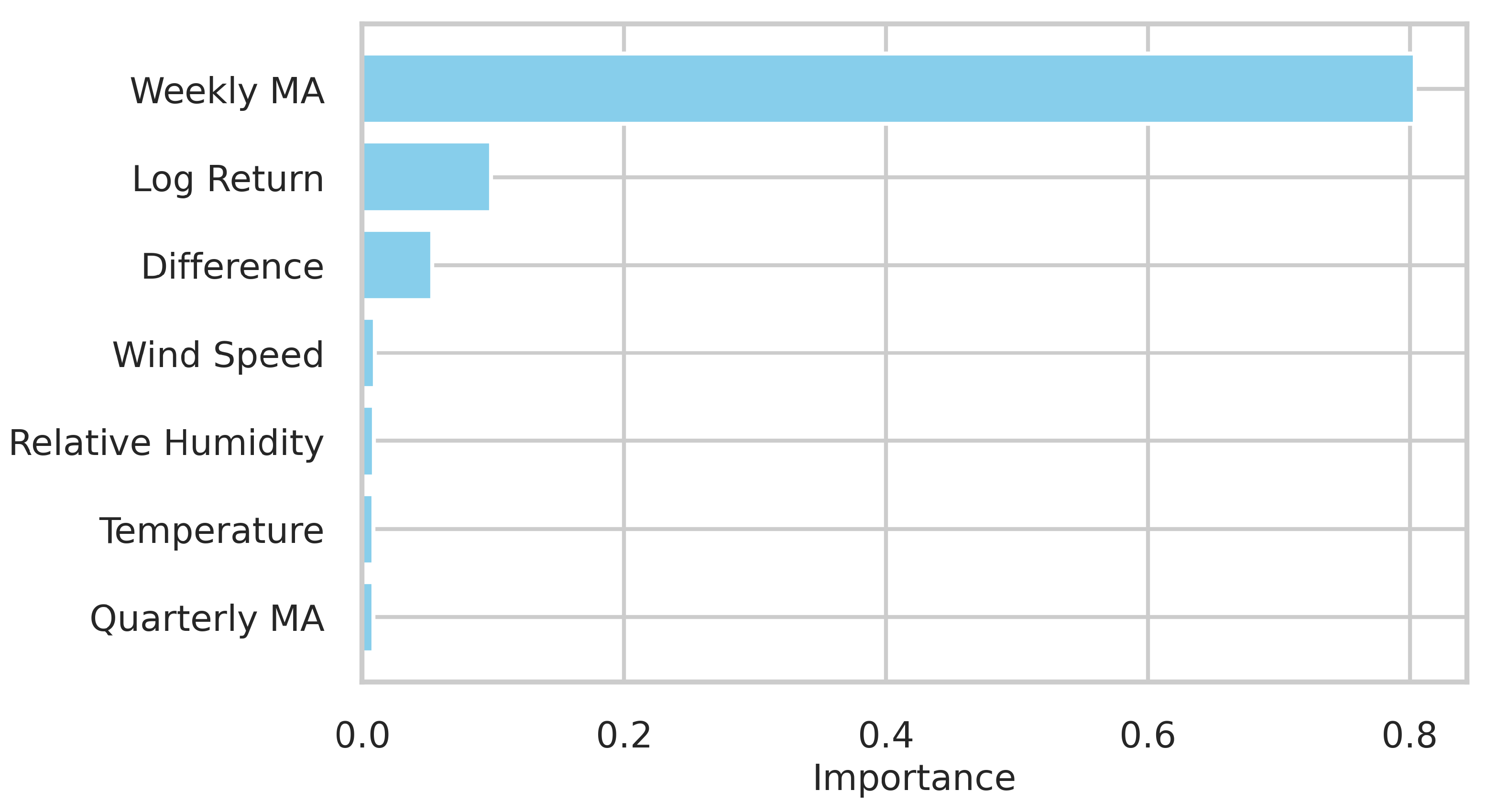
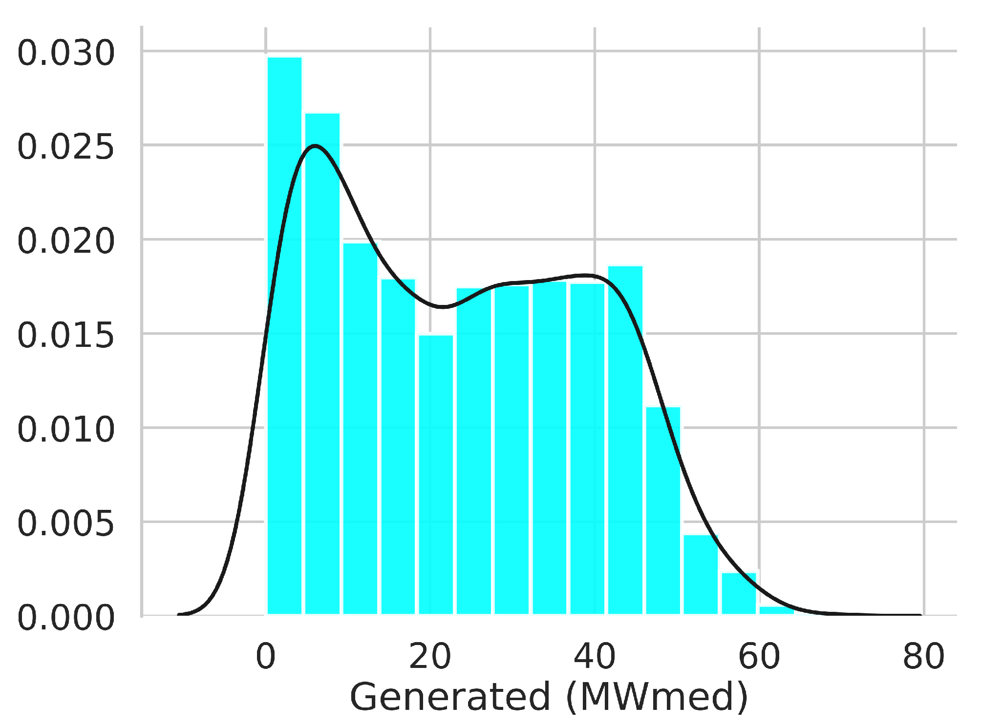
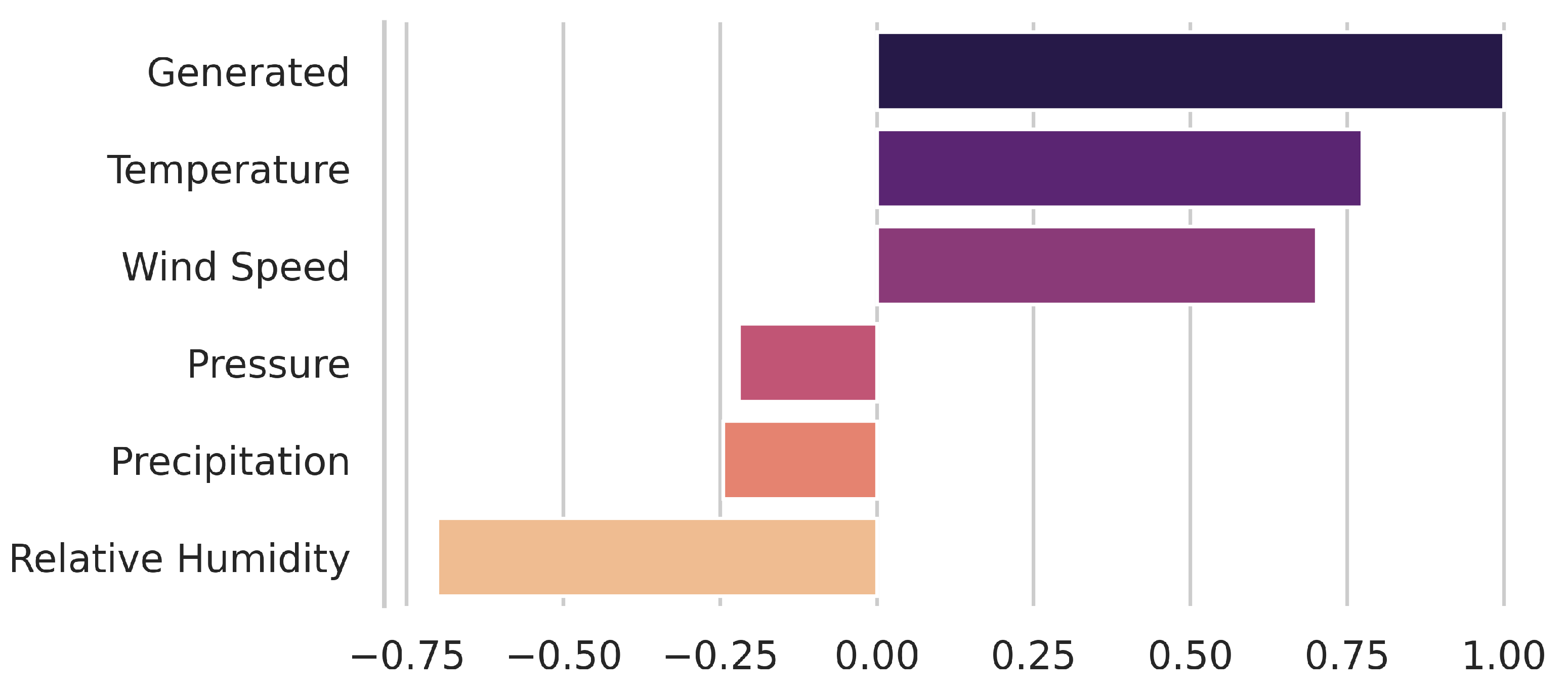
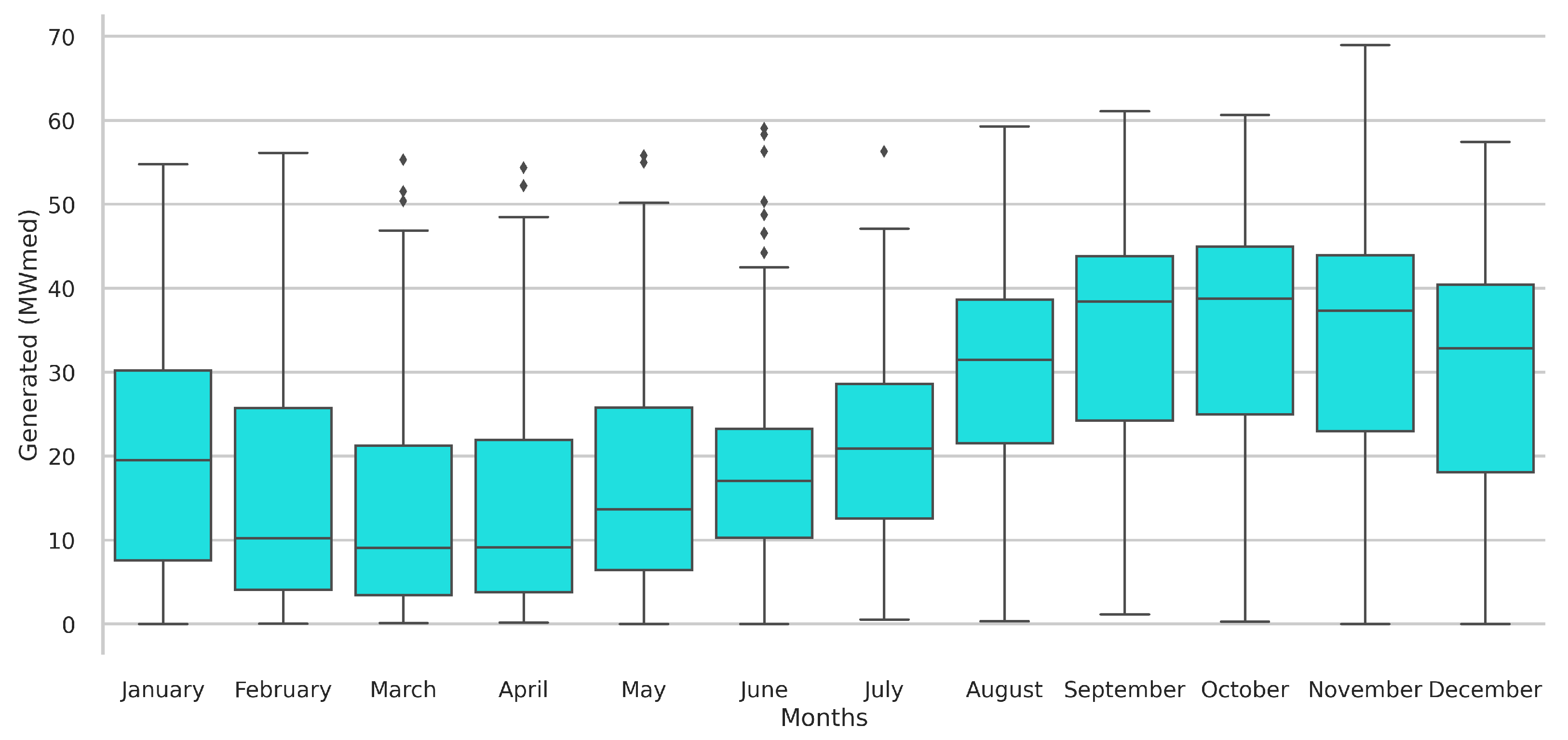
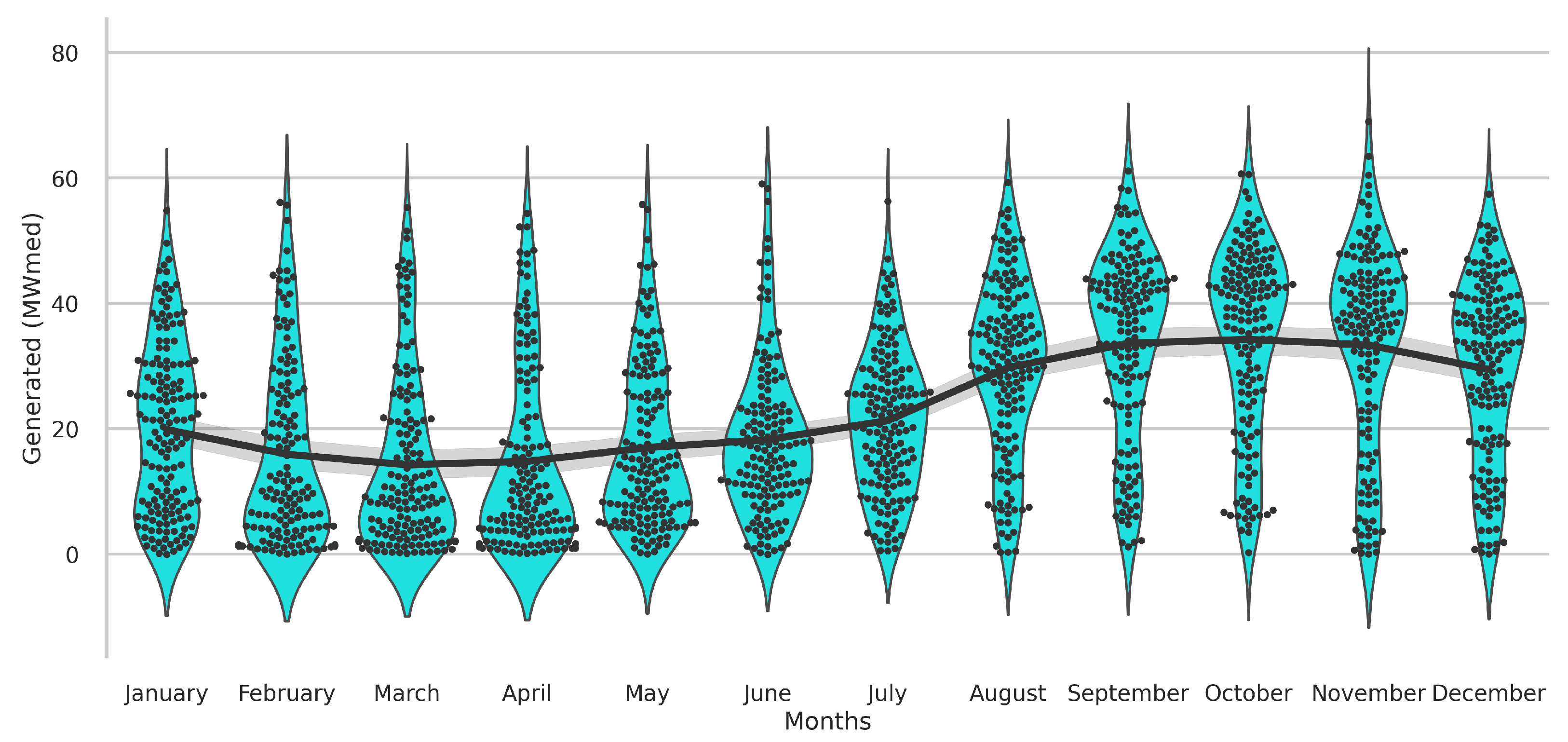
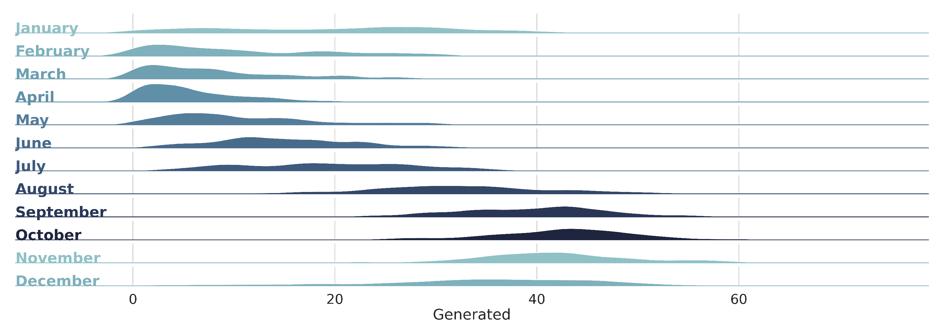
The knowledge data discovery study unlocked valuable insights into the relationship between regional weather conditions and local energy generation. By exploiting the correlation of weather-type features with wind energy, the convergence of the machine intelligence models was enhanced, while still comprehending the role of each variable in power generation. In particular, it was found that temperature, relative humidity and wind speed are the features that have the most significant impact on electricity production at the Praia Formosa wind complex. Another finding is that the generation at the investigated wind park is higher from August to November.

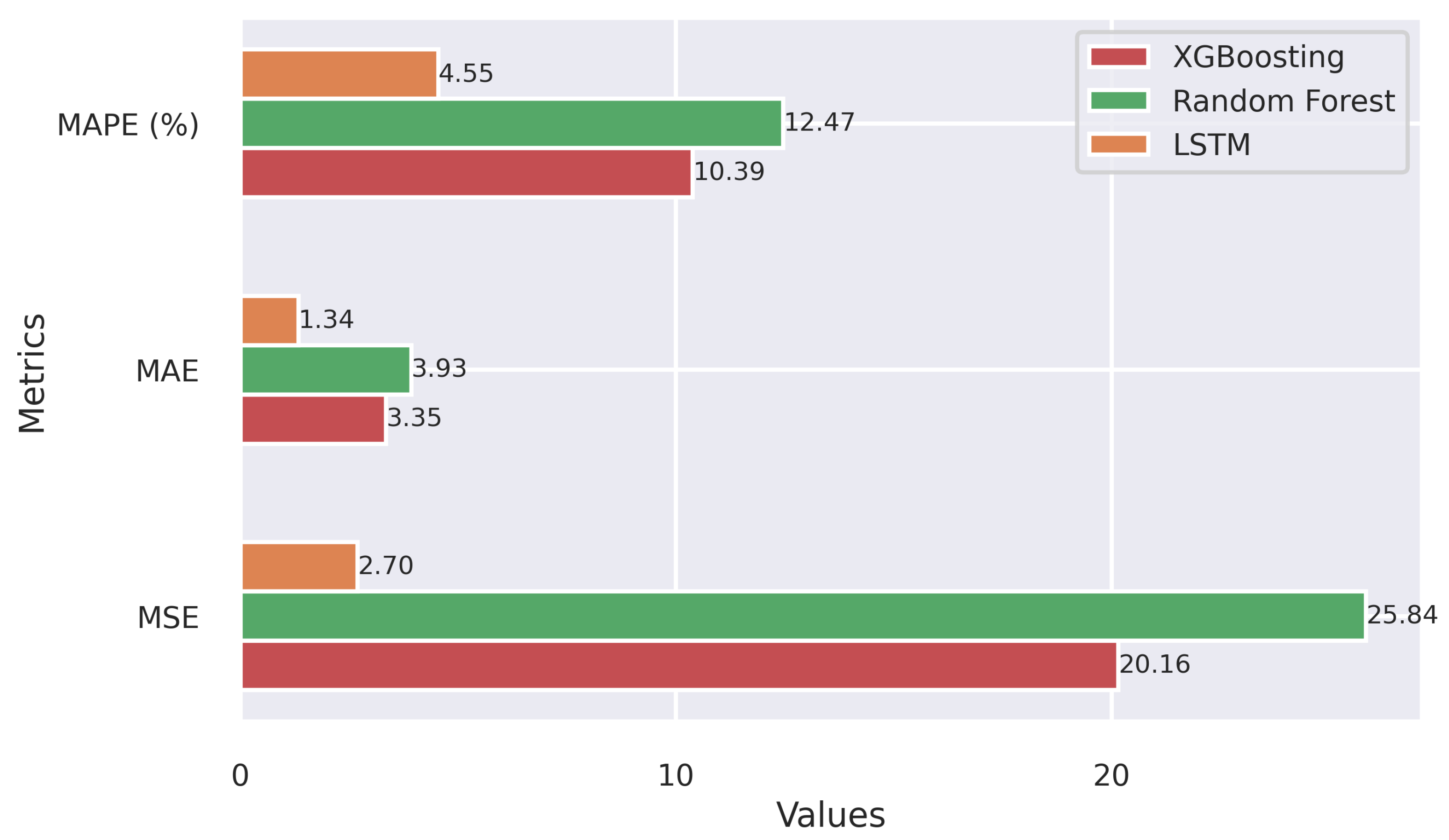
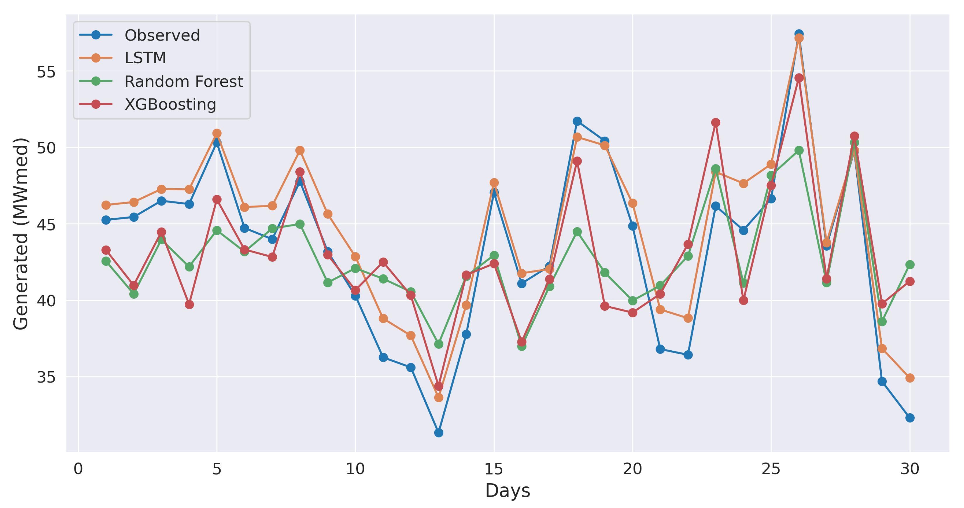
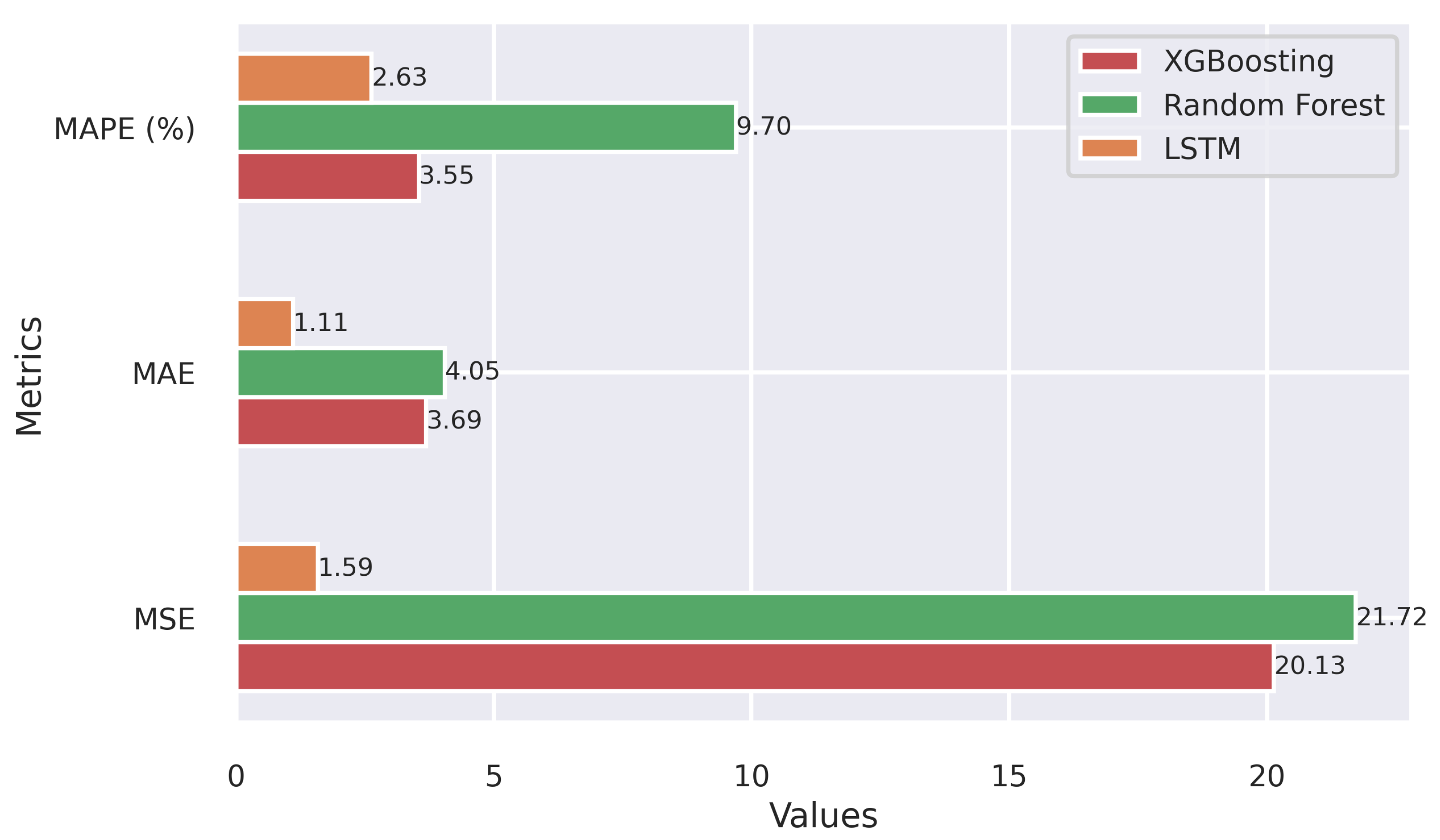
Wind power forecasting conducted over long-term windows, as explored in this paper, can assist power dispatch control not only in the northeastern region, but also throughout the whole country, such as through the National Interconnected System [64], as the machine intelligence models demonstrated a good accuracy rate over a full year. While both ensemble-type models, XGB and RF, delivered satisfactory results in terms of the MAPE and MSE metrics, LSTM stands out as the superior choice. The LSTM-based framework exhibited high accuracy, achieving a MAPE score of 4.55%. The forecasting plots for the last month of 2022 attested to the models’ capability to closely mirror actual energy generation, with LSTM excelling in capturing complex patterns.

Concerning the computational efficiency of the implemented models, it was observed that XGB reached the fastest processing time among the evaluated methods during the training phase. However, in the testing stage, the computational demand was notably reduced for all methods, with the LSTM-based model displaying the fastest inference time, completing the task in only 0.95 s. These results highlighted the potential use of the implemented machine intelligence methods for further applications in wind energy forecasting, contingent upon the availability of relevant data and tailored adjustments for different wind farm scenarios.

Apart from introducing a new methodological framework for forecasting energy generation in large-scale wind farms and conducting in-depth analyses of the gathered data, this study offers a comprehensive database sourced from multiple official Brazilian agencies. It caters to the needs of both the industry and researchers interested in investigating wind generation in large-scale parks, with a particular focus on the Brazilian context.

References

1. GWEC. Global Wind Report 2023; GWEC: Brussels, Belgium, 2023. [Google Scholar]
2. Nazir, M.S.; Bilal, M.; Sohail, H.M.; Liu, B.; Chen, W.; Iqbal, H.M. Impacts of renewable energy atlas: Reaping the benefits of renewables and biodiversity threats. Int. J. Hydrogen Energy 2020, 45, 22113–22124. [Google Scholar] [CrossRef]
3. Olabi, A.G.; Obaideen, K.; Abdelkareem, M.A.; AlMallahi, M.N.; Shehata, N.; Alami, A.H.; Mdallal, A.; Hassan, A.A.M.; Sayed, E.T. Wind Energy Contribution to the Sustainable Development Goals: Case Study on London Array. Sustainability 2023, 15, 4641. [Google Scholar] [CrossRef]
4. IRENA. Renewable Power Generation Costs in 2020. 2021. Available online: https://www.irena.org/publications/2021/Apr/Renewable-Power-Costs-in-2020 (accessed on 5 May 2023).
5. Wolniak, R.; Skotnicka-Zasadzień, B. Development of Wind Energy in EU Countries as an Alternative Resource to Fossil Fuels in the Years 2016–2022. Resources 2023, 12, 96. [Google Scholar] [CrossRef]
6. Fidalgo, J.N.; Matos, M.A. Forecasting Portugal Global Load with Artificial Neural Networks. In Proceedings of the Artificial Neural Networks (ICANN), Porto, Portugal, 9–13 September 2007; pp. 728–737. [Google Scholar]
7. Zheng, H.; Wu, Y. A XGBoost Model with Weather Similarity Analysis and Feature Engineering for Short-Term Wind Power Forecasting. Appl. Sci. 2019, 9, 3019. [Google Scholar] [CrossRef]
8. Demolli, H.; Dokuz, A.S.; Ecemis, A.; Gokcek, M. Wind power forecasting based on daily wind speed data using machine learning algorithms. Energy Convers. Manag. 2019, 198, 111823. [Google Scholar] [CrossRef]
9. Acaroğlu, H.; Márquez, F.P.G. Comprehensive Review on Electricity Market Price and Load Forecasting Based on Wind Energy. Energy Convers. Manag. 2021, 14, 7473. [Google Scholar] [CrossRef]
10. Qian, W.; Sui, A. A novel structural adaptive discrete grey prediction model and its application in forecasting renewable energy generation. Expert Syst. Appl. 2021, 186, 115761. [Google Scholar] [CrossRef]
11. Leme, J.V.; Casaca, W.; Colnago, M.; Dias, M.A. Towards Assessing the Electricity Demand in Brazil: Data-Driven Analysis and Ensemble Learning Models. Energies 2020, 13, 1407. [Google Scholar] [CrossRef]
12. Paula, M.; Colnago, M.; Fidalgo, J.N.; Wallace, C. Predicting Long-Term Wind Speed in Wind Farms of Northeast Brazil: A Comparative Analysis Through Machine Learning Models. IEEE Lat. Am. Trans. 2020, 18, 2011–2018. [Google Scholar] [CrossRef]
13. Li, J.; Armandpour, M. Deep Spatio-Temporal Wind Power Forecasting. In Proceedings of the IEEE International Conference on Acoustics, Speech and Signal Processing (ICASSP), Singapore, 23–27 May 2022; pp. 4138–4142. [Google Scholar]
14. Singh, U.; Rizwan, M.; Alaraj, M.; Alsaidan, I. A machine learning-based gradient boosting regression approach for wind power production forecasting: A step towards smart grid environments. Energies 2021, 14, 5196. [Google Scholar] [CrossRef]
15. Optis, M.; Perr-Sauer, J. The importance of atmospheric turbulence and stability in machine-learning models of wind farm power production. Renew. Sustain. Energy Rev. 2019, 112, 27–41. [Google Scholar] [CrossRef]
16. Li, L.L.; Zhao, X.; Tseng, M.L.; Tan, R.R. Short-term wind power forecasting based on support vector machine with improved dragonfly algorithm. J. Clean. Prod. 2020, 242, 118447. [Google Scholar] [CrossRef]
17. Malska, W.; Mazur, D. Electric energy production in a wind farm—The statistical analysis of measurement results using the time series. In Proceedings of the Progress in Applied Electrical Engineering (PAEE), Koscielisko, Poland, 25–30 June 2017; pp. 1–5. [Google Scholar]
18. Shabbir, N.; Kütt, L.; Jawad, M.; Amadiahanger, R.; Iqbal, M.N.; Rosin, A. Wind Energy Forecasting Using Recurrent Neural Networks. In Proceedings of the Big Data, Knowledge and Control Systems Engineering (BdKCSE), Sofia, Bulgaria, 21–22 November 2019; pp. 1–5. [Google Scholar]
19. Najeebullah, A.Z.; Khan, A.; Javed, S.G. Machine Learning based short term wind power prediction using a hybrid learning model. Comput. Electr. Eng. 2015, 45, 122–133. [Google Scholar] [CrossRef]
20. Puri, V.; Kumar, N. Wind energy forecasting using artificial neural network in Himalayan region. Model. Earth Syst. Environ. 2022, 8, 59–68. [Google Scholar] [CrossRef]
21. Solari, G.; Repetto, M.P.; Burlando, M.; De Gaetano, P.; Pizzo, M.; Tizzi, M.; Parodi, M. The wind forecast for safety management of port areas. J. Wind. Eng. Ind. Aerodyn. 2012, 104–106, 266–277. [Google Scholar] [CrossRef]
22. Cheng, W.Y.; Liu, Y.; Bourgeois, A.J.; Wu, Y.; Haupt, S.E. Short-term wind forecast of a data assimilation/weather forecasting system with wind turbine anemometer measurement assimilation. Renew. Energy 2017, 107, 340–351. [Google Scholar] [CrossRef]
23. Vaitheeswaran, S.S.; Ventrapragada, V.R. Wind Power Pattern Prediction in time series measuremnt data for wind energy prediction modelling using LSTM-GA networks. In Proceedings of the International Conference on Computing, Communication and Networking Technologies (ICCCNT), Kanpur, India, 6–8 July 2019; pp. 1–5. [Google Scholar]
24. Jaseena, K.; Kovoor, B.C. Deep learning based multi-step short term wind speed forecasts with LSTM. In Proceedings of the International Conference on Data Science, E-Learning and Information Systems, Dubai, United Arab Emirates, 2–5 December 2019; pp. 1–6. [Google Scholar]
25. Sowmya, C.; Kumar, A.G.; Kumar, S.S. Stacked LSTM recurrent neural network: A deep learning approach for short term wind speed forecasting. In Proceedings of the 2021 International Conference on Intelligent Technologies (CONIT), Hubli, India, 25–27 June 2021; pp. 1–7. [Google Scholar]
26. Papazek, P.; Schicker, I. A deep learning LSTM forecasting approach for renewable energy systems. EGU Gen. Assem. 2021, 2021, 19–30. [Google Scholar]
27. Ziaei, D.; Goudarzi, N. Short-Term Wind Characteristics Forecasting Using Stacked LSTM Networks. In Proceedings of the ASME Power Conference, Virtual, 20–22 July 2021; Volume 85109, p. V001T09A013. [Google Scholar]
28. Kumar, D.; Mathur, H.; Bhanot, S.; Bansal, R.C. Forecasting of solar and wind power using LSTM RNN for load frequency control in isolated microgrid. Int. J. Model. Simul. 2021, 41, 311–323. [Google Scholar] [CrossRef]
29. Wilczak, J.; Finley, C.; Freedman, J.; Cline, J.; Bianco, L.; Olson, J.; Djalalova, I.; Sheridan, L.; Ahlstrom, M.; Manobianco, J.; et al. The Wind Forecast Improvement Project (WFIP): A Public–Private Partnership Addressing Wind Energy Forecast Needs. Bull. Am. Meteorol. Soc. 2015, 96, 1699–1718. [Google Scholar] [CrossRef]
30. Mesa-Jiménez, J.; Tzianoumis, A.; Stokes, L.; Yang, Q.; Livina, V. Long-term wind and solar energy generation forecasts, and optimisation of Power Purchase Agreements. Energy Rep. 2023, 9, 292–302. [Google Scholar] [CrossRef]
31. Wang, X.; Liu, Y.; Hou, J.; Wang, S.; Yao, H. Medium- and Long-Term Wind-Power Forecasts, Considering Regional Similarities. Atmosphere 2023, 14, 430. [Google Scholar] [CrossRef]
32. Jørgensen, K.L.; Shaker, H.R. Wind Power Forecasting Using Machine Learning: State of the Art, Trends and Challenges. In Proceedings of the IEEE International Conference on Smart Energy Grid Engineering (SEGE), Oshawa, ON, Canada, 12–14 August 2020; pp. 44–50. [Google Scholar]
33. EPE Brazil. Empresa de Pesquisa Energetica. 2022. Available online: https://www.epe.gov.br/en/publications/publications/brazilian-energy-balance (accessed on 8 January 2023).
34. SIIF Praia Formosa Wind Farm. Global Wind Power Tracker Project. 2023. Available online: https://www.gem.wiki/SIIF_Praia_Formosa_wind_farm (accessed on 3 February 2023).
35. Ribeiro, R.; Fanzeres, B. Identifying Representative Days of Wind Speed in Brazil Using Machine Learning Techniques. In Proceedings of the 2022 IEEE Power & Energy Society General Meeting (PESGM), Denver, CO, USA, 17–21 July 2022; pp. 1–5. [Google Scholar]
36. Gilliland, J.M.; Keim, B.D. Position of the South Atlantic Anticyclone and its impact on surface conditions across Brazil. J. Appl. Meteorol. Climatol. 2018, 57, 535–553. [Google Scholar] [CrossRef]
37. de Almeida Yanaguizawa Lucena, J.; Lucena, K.A.A. Wind energy in Brazil: An overview and perspectives under the triple bottom line. Clean Energy 2019, 3, 69–84. [Google Scholar] [CrossRef]
38. GWA. Global Wind Atlas. 2023. Available online: https://globalwindatlas.info/ (accessed on 8 January 2023).
39. ONS Brazil. National Electrical System Operator. 2022. Available online: http://ons.org.br (accessed on 3 November 2022).
40. INMET Brazil. National Institute of Meteorology. 2023. Available online: http://www.inmet.gov.br/portal/index.php?r=home2/index (accessed on 3 January 2023).
41. Lee, J.; Wang, W.; Harrou, F.; Sun, Y. Wind power prediction using ensemble learning-based models. IEEE Access 2020, 8, 61517–61527. [Google Scholar] [CrossRef]
42. Chen, T.; Guestrin, C. XGBoost: A Scalable Tree Boosting System. In Proceedings of the ACM SIGKDD International Conference on Knowledge Discovery and Data Mining, San Francisco, CA, USA, 13–17 August 2016; pp. 785–794. [Google Scholar] [CrossRef]
43. Bentéjac, C.; Csörgo, A.; Martínez-Muñoz, G. A comparative analysis of gradient boosting algorithms. Artif. Intell. Rev. 2021, 54, 1937–1967. [Google Scholar] [CrossRef]
44. Wade, C. Hands-on Gradient Boosting with XGBoost and Scikit-Learn: Perform Accessible Machine Learning and Extreme Gradient Boosting with Python; Packt Publishing: Birmingham, UK, 2020. [Google Scholar]
45. Munir, S.; Seminar, K.B.; Sudradjat; Sukoco, H.; Buono, A. The Use of Random Forest Regression for Estimating Leaf Nitrogen Content of Oil Palm Based on Sentinel 1-A Imagery. Information 2022, 14, 10. [Google Scholar] [CrossRef]
46. Dudek, G. A Comprehensive Study of Random Forest for Short-Term Load Forecasting. Energies 2022, 15, 7547. [Google Scholar] [CrossRef]
47. Hewamalage, H.; Bergmeir, C.; Bandara, K. Recurrent Neural Networks for Time Series Forecasting: Current status and future directions. Int. J. Forecast. 2021, 37, 388–427. [Google Scholar] [CrossRef]
48. Mahjoub, S.; Chrifi-Alaoui, L.; Marhic, B.; Delahoche, L. Predicting Energy Consumption Using LSTM, Multi-Layer GRU and Drop-GRU Neural Networks. Sensors 2022, 22, 4062. [Google Scholar] [CrossRef]
49. Han, S.; Qiao, Y.H.; Yan, J.; Liu, Y.Q.; Li, L.; Wang, Z. Mid-to-long term wind and photovoltaic power generation prediction based on copula function and long short term memory network. Appl. Energy 2019, 239, 181–191. [Google Scholar] [CrossRef]
50. Malhan, P.; Mittal, M. A novel ensemble model for long-term forecasting of wind and hydro power generation. Energy Convers. Manag. 2022, 251, 114983. [Google Scholar] [CrossRef]
51. Pedregosa, F.; Varoquaux, G.; Gramfort, A.; Michel, V.; Thirion, B.; Grisel, O.; Blondel, M.; Prettenhofer, P.; Weiss, R.; Dubourg, V.; et al. Scikit-learn: Machine Learning in Python. J. Mach. Learn. Res. 2011, 12, 2825–2830. [Google Scholar]
52. Keitsch, K.A.; Bruckner, T. Input data analysis for optimized short term load forecasts. In Proceedings of the IEEE Innovative Smart Grid Technologies-Asia (ISGT-Asia), Melbourne, Australia, 28 November–1 December 2016; pp. 1–6. [Google Scholar]
53. de Myttenaere, A.; Golden, B.; Le Grand, B.; Rossi, F. Mean Absolute Percentage Error for regression models. Neurocomputing 2016, 192, 38–48. [Google Scholar] [CrossRef]
54. Yang, Y.; Han, L.; Wang, Y.; Wang, J. China’s energy demand forecasting based on the hybrid PSO-LSSVR model. Wirel. Commun. Mob. Comput. 2022, 2022, 7584646. [Google Scholar] [CrossRef]
55. Hudson, R.S.; Gregoriou, A. Calculating and comparing security returns is harder than you think: A comparison between logarithmic and simple returns. Int. Rev. Financ. Anal. 2015, 38, 151–162. [Google Scholar] [CrossRef]
56. Chen, B.; Choi, J.; Escanciano, J.C. Testing for fundamental vector moving average representations. Quant. Econ. 2017, 8, 149–180. [Google Scholar] [CrossRef]
57. Dahouda, M.K.; Joe, I. A deep-learned embedding technique for categorical features encoding. IEEE Access 2021, 9, 114381–114391. [Google Scholar] [CrossRef]
58. Saarela, M.; Jauhiainen, S. Comparison of feature importance measures as explanations for classification models. SN Appl. Sci. 2021, 3, 272. [Google Scholar] [CrossRef]
59. Li, X.; Chen, W.; Zhang, Q.; Wu, L. Building auto-encoder intrusion detection system based on random forest feature selection. Comput. Secur. 2020, 95, 101851. [Google Scholar] [CrossRef]
60. Bergstra, J.; Bengio, Y. Random Search for Hyper-Parameter Optimization. J. Mach. Learn. Res. 2012, 13, 281–305. [Google Scholar]
61. Stekhoven, D.J.; Bühlmann, P. MissForest—Non-parametric missing value imputation for mixed-type data. Bioinformatics 2012, 28, 112–118. [Google Scholar] [CrossRef] [PubMed]
62. Zhang, S.; Gong, L.; Zeng, Q.; Li, W.; Xiao, F.; Lei, J. Imputation of gps coordinate time series using missforest. Remote Sens. 2021, 13, 2312. [Google Scholar] [CrossRef]
63. Hanifi, S.; Liu, X.; Lin, Z.; Lotfian, S. A critical review of wind power forecasting methods—Past, present and future. Energies 2020, 13, 3764. [Google Scholar] [CrossRef]
64. García, C.L.; Grimoni, J.A.B.; Morales Udaeta, M.E. Integrating Wind Power to the National Interconnected System in Brazil. Int. J. Electr. Energy 2016, 4, 48–53. [Google Scholar] [CrossRef]
Figure 1. Wind speed average in Brazil (Source: Global Wind Atlas [38]).
Inventions 08 00126 g001
Figure 2. Location of the Praia Formosa wind complex and its aerogenerators.
Inventions 08 00126 g002
Figure 3. Feature importance using a Random-Forest-based approach.
Inventions 08 00126 g003
Figure 4. Energy generation histogram and the Kernel Density Estimate curve. The x-axis groups the energy generated (in MWmed), while the y-axis quantifies the probability density values.
Inventions 08 00126 g004
Figure 5. Correlation computed for the main collected variables.
Inventions 08 00126 g005
Figure 6. Boxplot of energy generated per day of the week.
Inventions 08 00126 g006
Figure 7. Boxplot of energy generated per month.
Inventions 08 00126 g007
Figure 8. Violin plot of the energy generated (MWmed) in a whole year, highlighting the asymmetric distribution of the data across different months.
Inventions 08 00126 g008
Figure 9. Facetgrid plot, composed of the stacked density plots of energy generated (MWmed) arranged by month.
Inventions 08 00126 g009
Figure 10. MAPE, MAE and MSE over the test data for the machine learning-based models built with optimized hyperparameters.
Inventions 08 00126 g010
Figure 11. Energy generated predictions for the last 30 days of 2022.
Inventions 08 00126 g011
Figure 12. Energy generated residues for the last 30 days of 2022.
Inventions 08 00126 g012
Figure 13. MAPE, MAE and MSE over the last 30 days of 2022.
Inventions 08 00126 g013