
Urban Planning of Coastal Adaptation under Sea-Level Rise: An Agent-Based Model in the VIABLE Framework


1
Climate Service Center Germany (GERICS), Helmholtz-Zentrum Hereon, Fischertwiete 1, 20095 Hamburg, Germany
2
Institute of Coastal Systems-Analysis and Modeling, Helmholtz-Zentrum Hereon, Max-Planck-Straße 1, 21502 Geesthacht, Germany
3
Research Group Climate Change and Security (CLISEC), Institute of Geography, Center for Earth System Research and Sustainability (CEN), Universität Hamburg, Grindelberg 5/7, 20144 Hamburg, Germany
*
Author to whom correspondence should be addressed.
Urban Sci. 2023, 7(3), 79; https://doi.org/10.3390/urbansci7030079
Submission received: 17 May 2023
/
Revised: 11 July 2023
/
Accepted: 12 July 2023
/
Published: 27 July 2023
(This article belongs to the Special Issue Coastal Urban Dynamics under Climate Change)
Abstract
:Coastal flood risk and sea-level rise require decisions on investment in coastal protection and, in some cases, the relocation of urban areas. Models that formalize the relations between flooding costs, protective investments, and relocation can improve the analysis of the processes and issues involved and help to support decision-making better. In this paper, an agent-based model of a coastal city is represented in NetLogo. This model is based on the VIABLE modeling framework and describes adaptive dynamic agent behavior in a changing system. The hypothetical city faces damage caused by gradually rising sea levels and subsequent extreme sea-level events. To mitigate these risks, an “urban planner” agent has two adaptation measures at their disposal: developing coastal defenses or, as a more extreme measure, relocating vulnerable areas inland. As the simulation progresses and the decisions change with rising sea levels, the agent alters investments in these two measures to increase its value function, resulting in dynamic reactive behavior. Additionally, gradual sea-level rise is implemented in various modes, along with extreme sea-level events that cause severe short-term damage. The results of simulations under these modes and with multiple scenarios of agent action are presented. On average, agent behavior is quite reactive under limited foresight. Individual simulations yield a ‘priming’ effect when comparing different timings of extreme sea-level events, wherein an earlier extreme event primes the agent to adapt and thus be better prepared for subsequent events. Agent success with adaptation is also found to be sensitive to the costs involved, and these varying degrees of adaptation success are quantified using three parameters of adaptation success.
1. Introduction
Urban areas represent a particularly interesting case for planning climate adaptation strategies. Since 2007, a majority of the world’s population has resided in urban areas [1], which is projected to continue to grow. Among cities, those residing on the coast are especially vulnerable to climate change impacts. As a result of climate change, the global mean sea level is projected to rise between 0.38–0.77 m by 2100 (the latter being the high greenhouse gas emission RCP 8.5 scenario [2]). This presents a risk to low-lying areas worldwide, particularly urban agglomerations on the coast, which represent greater exposure due to higher population density. Aside from the direct hazard posed by sea-level rise, another consequence is more frequent and severe extreme sea-level events caused by storm surges brought on by tropical storms and cyclones, which presents another greater hazard to urban coastal areas [2]. For instance, storm surges and extreme sea-level events can lead to flooding when they exceed the flood protection of such urban areas. As a result, the importance of planning and managing climate change adaptation in urban coastal areas is well recognized in the adaptation literature [3].
Planning adaptation strategies in coastal cities to manage increasing risk requires transdisciplinary modeling approaches that can account for complex urban dynamics in addition to the impacts of climate change. Agent-based modeling (ABM) is particularly well-suited for this purpose, with individual decision rules applied to autonomous agents leading to complex emergent patterns [4,5]. In the urban coastal environment, ABM is used to model human responses across multiple spatial and temporal scales to better plan risk reduction and adaptation, particularly for flood risks. Such social simulation approaches can be used to build a comprehensive, complex, and behaviorally rich model that forms the basis for a better understanding of the dynamics and decision processes involved in coastal planning. In addition, such tools can help urban planners and managers of coastal protection create potential scenarios and explore possible adaptation pathways.
For instance, Yang et al. [6] used the ABM approach to model human responses at the household level to a flood incident and assess losses. Dawson et al. [7] modeled the vulnerability of agents at the individual level to calculate risk and plan flood incident management. A review by Taberna et al. [8] found two schools of flood management research that employed ABM: one focusing on the hazard and vulnerability aspects of risk that aimed to calculate expected annual damages, and the other focusing more on the exposure aspect, modeling urban land use and market dynamics that affect values at risk. Our work broadly falls into the latter category, characterized by the presence of endogenous urban relocation. However, it also incorporates elements commonly observed in the former category, such as temporally varying exogenous hazards due to climate change. Therefore, our work serves as a much-needed bridge between these two modeling schools. In addition, we aim to provide a tool to extend this area of urban flood risk research with a transdisciplinary approach.
In this paper, we apply agent-based modeling to the idealized case of a hypothetical generalized coastal city. Specifically, we employ the VIABLE (Values and Investments in Agent-Based Interaction and Learning in Environmental Systems) agent-based modeling framework [9]. This framework has been applied in multiple contexts across various scales. The ABM outlined by Yang et al. [10] is an example of a local-scale application within a single urban area. The model describes a small number of commuters seeking optimal travel pathways through a city. In contrast, other model applications to bioenergy, land use, and fisheries [9] apply the ABM framework at subnational and international scales with much larger numbers of interacting agents. We apply this framework to a hypothetical coastal city whose adaptation options are governed by a single agent. We use it to form a complex decision framework for this agent that dynamically responds to increased flood hazards posed by sea-level rise. Additionally, we illustrate its usage for modeling two alternative adaptation strategies for a coastal city.
2. Materials and Methods
2.1. Agent-Based Modelling
The modeling approach employed here is agent-based modeling (ABM) within the VIABLE modeling framework (see the next section). ABM approaches generally involve multiple autonomous individuals acting on certain rules. These rules govern their interactions with the environment in which they reside and with other agents within that environment. ABM comprises rules applied across smaller (individual) scales that result in aggregated behavior at larger (population) scales.
A common aspect of these models is that applying simple rules to multiple agents results in complex emergent behavior at larger scales, such as in the famous cases of Thomas Schelling’s models of segregation [4] and James M. Sakoda’s checkerboard model of social interaction [5]. ABM is greatly aided by the increased computational resources available in the digital age, allowing more detailed rules to be implemented across larger agent populations and shorter computation times. As a result, ABM can now facilitate multiple simulations under different assumptions and scenarios.
2.2. The VIABLE Framework
We build our model using the VIABLE agent-based modeling framework [5]. This framework is based on viability theory, which describes conditions for bounding systems to an area where they are “viable,” termed their viability domain. For example, the global climate system could be limited by global mean surface temperature change, such as the 1.5 to 2 degrees target defined in the 2015 Paris Agreement, within which the system is considered viable. Agents in these dynamic systems follow “adaptive control,” which means they possess limited capabilities in terms of resources and knowledge (bounded rationality). They use strategic decision rules to adapt to the changing environment and stay within their viability domain.
The VIABLE framework formalizes the dynamics of an agent using adaptive control to stay within its viability domain. Agents seek to achieve target states by acting on the system to alter its state by investing their capital into multiple action pathways. A value–cost function determines how effective the agent’s actions are. Using certain decision rules, the agent evaluates the changes in the system and alters how it invests its capital accordingly. The framework also models the dynamic interactions between agents, allowing for the study of the emergence of conflict or cooperation. In this study, we employ only single-agent action in the VIABLE framework.
2.3. The Single-Agent Urban Coastal Model
The agent in the model represents an urban planner tasked with managing a coastal city. The city is the system that the agent interacts with and generates income through revenues for the agent. In the current model version, it is represented in a non-spatially explicit form. A fraction of the area is designated as the coastal territory (50% for this study), with the rest of the city’s territory being inland. The coastal territory of the city generates more value per unit area than the inland territory (taken to be twice the value). However, it is vulnerable to coastal flooding hazards resulting from sea-level rise and extreme events.
To avoid damages from these coastal hazards, the urban planner is presented with two options for adaptation action: it can either build up the city’s coastal defenses or, as a more extreme measure, relocate vulnerable parts of the urban territory inland. In keeping with the VIABLE model, these action paths represent the primary mechanism of agency for this planner. The planner can allocate any amount of the income it gains from the city as investments in the adaptation measures. Certain fractions of the invested income allocated to each adaptation option depend on the agent’s decision rules. The amount remaining after the investment is consumed by the agent and counts towards its utility. The fraction of investment allocated to each path is based on a set of variables termed the agent’s priority for that path. It is also possible for the agent to refrain from any investment at all and consume all generated value.
Therefore, the agent can have two control variables: the total amount of capital invested and the fraction of invested capital going to one of the options (since there are only two options, the fraction allocated to the other derives from this value). At every timestep of the simulation, the agent can alter its control variables based on its evaluation of the current state of the system. Essentially, the agent seeks to increase or maximize its value function and will alter these control variables in the direction that leads to the highest value.
Sea-level rise is present in the model as a prescribed external force. The sea level is set to its initial (reference) value at the start of the model simulation, which gradually rises over time as the simulation progresses. Without any adaptation actions, damages are incurred to the city based on what fraction of the urban territory is coastal. However, if the agent develops coastal defenses through investment, sea-level rise-related damages are reduced. Coastal defenses are represented in our model in terms of their “efficient height,” which represents the maximum sea level that they can protect against. On the other hand, when the agent invests in relocation, the damages are also reduced since a smaller share of the area that generates income is located in the coastal territory of the city.
2.4. Mathematical Formulation of the Model
2.4.1. Agent Dynamics
The agent seeks to increase and, as far as possible, optimize its value function V, which is a balance between positive utility U and disutility W. Within the framework of a basic economic model, utility is a function of consumption, which, as stated earlier, corresponds to the capital remaining after investments are deducted. In contrast, disutility is a function of damages incurred by the city.
Therefore, the value is given as:
where K is the capital available to the agent and C is the total amount invested. Since all resources remaining after investment are consumed by the agent and do not carry over to the next timestep, the capital K available to the agent at any time is equal to the total income Y generated by the city in that timestep:
This gives us the following value equation:
The utility and disutility functions are taken to be of a standard non-linear form, as used in many economic models:
where α and β are constants, such that and is a parameter describing the relative importance of negative utility from damages with respect to positive utility from consumption.
The income Y, generated by the city, is given as:
where Bc is the income generated per unit coastal urban area (Sc being the total coastal urban area) and BI is the income generated per unit inland urban area (SI being the inland urban area). We set Bc > BI, i.e., the coastal area of the city is more valuable per unit area, as mentioned earlier.
2.4.2. Agent Investments (Optimizing Behavior)
The total amount invested C and the fraction of it that is invested in coastal defenses r are the two control variables of the agent. Since there are two investment pathways, the fraction invested in coastal relocation is 1-r. So, following the optimizing version of the VIABLE framework, at every timestep, the agent sets target values for its control variables, C* and r*, that correspond to the maximum attainable value, V*. The process of computing the optimal value is detailed further in Appendix B. It then alters the current values of the control variables by ΔC and Δr in the direction of these target values. Therefore, these delta values are proportional to the difference between the target and current values.
The process of altering these control variables is regulated by variables representing the agent’s adaptation rate (kC for ΔC and α for Δr). The adaptation rate ensures the agent cannot instantaneously move to the optimum state. The dynamics of ΔC are further regulated by the terms C and (Y − C), ensuring that the change slows down as C approaches the maximum value Y and the minimum value 0.
After C has been altered by ΔC and r by Δr, the investments in each pathway would be:
2.4.3. State Dynamics
Towards the end of each timestep, the state variables change in response to these investments after the agent has allocated them.
The coastal area Sc decreases if any investments in relocation have been made:
where kR is the efficiency of investments in urban relocation. The inland area SI increases by an equivalent amount, depending on the investment allocated by the agent to urban relocation.
As described by Kind [11], investments in coastal defenses occur periodically, with the agent evaluating these investments and reallocating them, if necessary, for a fixed period. In our model, we assume this is conducted every five years, reflecting public investment policies in several countries. The amount invested is then split into five equal amounts that are invested over the next five years to represent the project of coastal defense heightening.
The damage-mitigating ability of coastal defenses is represented by their “effective height,” H*, which is the maximum sea level they can effectively protect against. This was changed based on the investment CH allocated to developing coastal defenses. Without investment, the defenses depreciate over time at the following depreciation rate λ:
where kH is the efficiency of investment in coastal protection.
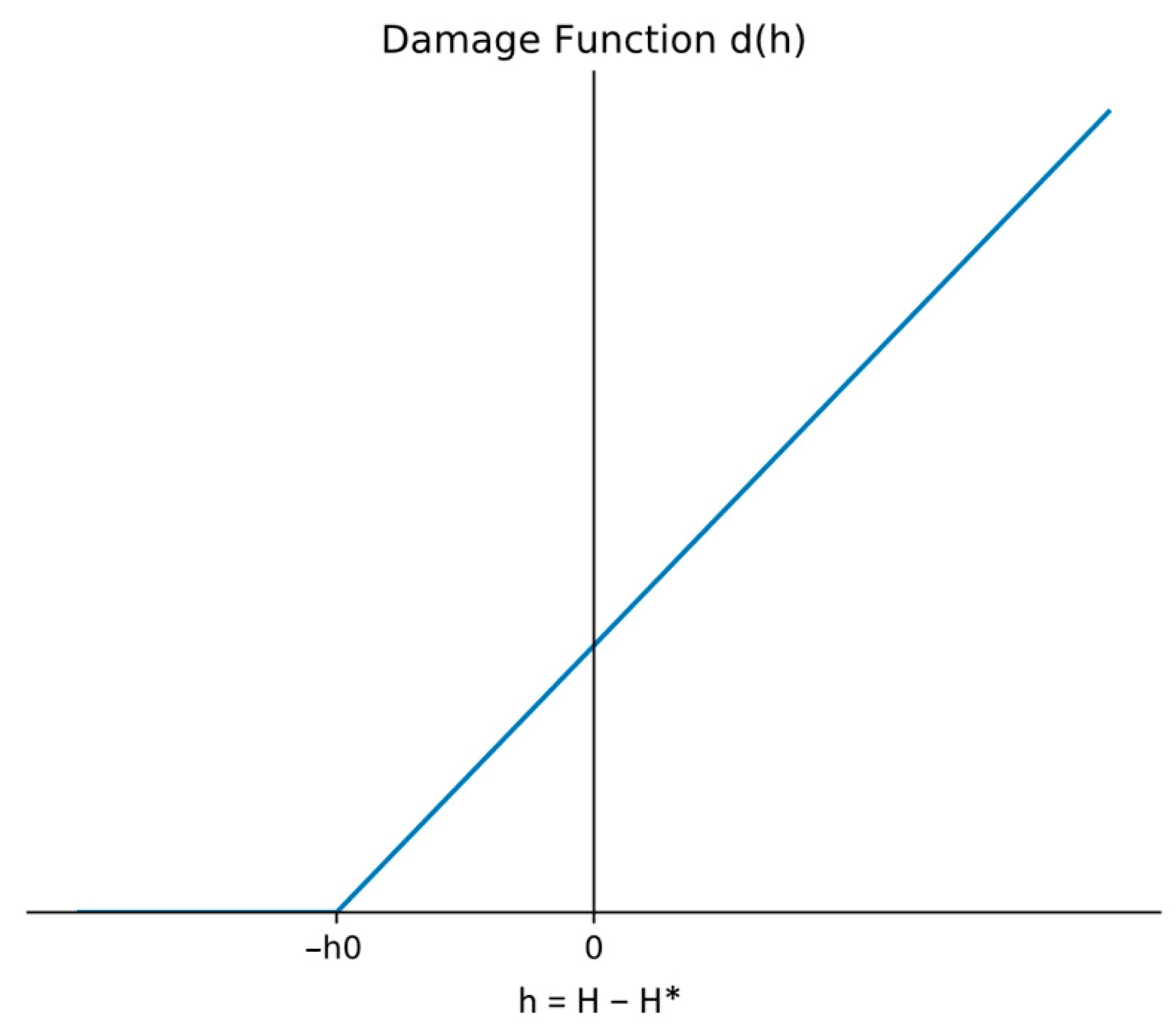
At this point, sea level H changes exogenously at discrete time points based on the timestep. We implement various modes of sea-level rise, primarily one where, after every five timesteps, the sea level increases by one height unit per step for the next five. If the sea level exceeds the effective height of the defenses, then damage is incurred to the city. This damage D is a function of the amount by which sea level H exceeds the effective defense height H*. We define a “minimum threshold height,” h0, which is how much higher than the sea level the coastal defense height should be to sustain zero damages. In practice, this means that a coastal planner will build a safety margin so that the effective height is always higher than the mean annual sea level. This also incorporates some reflection on extreme events, depending on the appreciation and acceptability of the flood risk (see also [12]). So, the damage function is zero when H* = H + h0 and increases linearly as H − H* increases. The damage is also proportional to the vulnerability of the coastal area SC.
The damage function , visually represented in Figure 1, therefore specifies the damage per unit of coastal urban area. It is zero until (H − H*) equals the minimum threshold height h0, which increases linearly.
2.4.4. Extreme Sea-Level Events
In addition to the baseline long-term gradual sea-level rise, we introduce “climate shocks,” short-term but large-scale perturbations to the sea level representing extreme sea-level events, such as storm surges caused by cyclone systems. The model includes a few different climate shock modes (Table 1). However, for the purposes of this paper, we use the so-called “probabilistic” mode, where the timing and severity of climate shocks are dependent on a percentage chance at each timestep. Over time, this chance increases, making shocks, on average, more frequent and severe in the later stages of the simulation, mirroring the projected effects of climate change on extreme sea-level events.
Besides providing a mechanism to better simulate the complexity of the urban coast, probabilistic climate shocks introduce an element of randomness to each simulation. This leads to more diverse agent behavior and provides another impetus for the agent to work toward climate adaptation.
2.4.5. Agent Action
As the simulation progresses, the agent observes sea-level changes and forms an approximate expectation for future sea levels. This is conducted by extrapolating linearly from all observed sea levels until the current time step. The agent’s expected sea level at the next investment period forms the basis for the targeted coastal defense height the agent wishes to achieve. The agent aims to reach a defense height corresponding to a level of protection that exceeds the expected sea level, and this built-in buffer height is defined based on the average sea level due to extreme events.
As this expected level is a linear extrapolation of past observed levels, a gradual rise would mean the agent expects an increased risk at the next investment period and prepares for it. Effectively, this also means that the agent decreases its expected risk at the next timestep in cases where the observed sea level does not change and may underestimate future sea levels.
Additionally, when the agent observes an extreme sea-level event, the expected risk is updated to the maximum level observed, and the agent seeks to ensure that an extreme event of a similar magnitude will not cause damage in the future. This represents the agent’s learning ability and, in effect, means that the agent prepares for the highest observed extreme sea-level event.
2.4.6. Investment Efficiency
The efficiencies of investments are important parameters for tuning the model to represent scenarios analogous to reality, as they signify the crucial link between agent action and the system’s response to this action. For clarity, the efficiency of an investment can be divided into two factors: Firstly, there is a fractional efficiency between 0 and 1, which represents how much of the invested capital is effectively utilized. Secondly, there is a cost conversion factor, or “cost factor,” which translates monetary units to height units (in the case of coastal defense development) or area units (for city relocation). In the first case, this cost factor represents how many centimeters the coastal defenses are heightened by for each euro spent, and in the second case, how many square kilometers of coastal territory are relocated inland for each euro spent.
The investment efficiencies and are both the product of a fractional efficiency and a cost factor:
Breaking down these factors allows us to separate two effects: the cost of the adaptation actions and the agents’ efficiency in implementing them. Different geographical areas can be represented by varying the former, where this factor is determined by differences in the costs of labor and materials in different locations. Different levels of efficiency in governance and adaptation plan implementation can be represented by varying the latter. The fractional efficiencies and can vary in value from 0 to 1, depending on the scenario. When the value is 1, all of the agent’s invested resources are allocated to the chosen adaptation path with 100% efficiency. For our simulations, we take a value of 50% efficiency for heightening coastal defenses (a sensitivity analysis for different values of this fractional efficiency is illustrated in Appendix A).
We base our estimates of coastal defense on cost factors from Jonkman et al. [13], where for a sample area in the Netherlands, the cost of developing coastal defenses is roughly approximated at 20 M € per m of coastal defense height per km of coastline. This yields the following value (in m/M €), dependent on coastline length, (km):
We denote this value as a “high-cost” scenario for coastal defenses, as opposed to a “low-cost” scenario where the cost factor (drawn from [13] for a sample area in Vietnam) is given as:
Therefore, we can see the effect of this cost factor by comparing these two scenarios.
On the other hand, the cost factor for coastal relocation is based on the income generated by the coastal tiles being relocated.
2.4.7. Units and Values of Model Parameters
3. Results
3.1. Agent Response
Broadly speaking, we observe the agent’s response to sea-level rise-related hazards as mostly reactive, as seen in the scenarios discussed below. With limited information and expectations based on a linear extrapolation of past observed sea levels, the agent primarily acts to mitigate damages that it anticipates in the next investment period. This means that during the simulation, the agent does not increase adaptation investment as long as expected damages are zero, i.e., the coastal defenses are sufficiently high to prevent sea-level rise.
When the agent does move towards adaptation, it heavily prefers the option of building coastal defenses (Figure 2). This preference for coastal defense development over city relocation can mostly be attributed to the setup of state dynamics. While coastal defenses serve as an efficient adaptation measure that sufficiently reduces damages related to sea-level rise, city relocation is a much more expensive process (represented in the model by the relocation investment efficiency parameter being much lower than the coastal defense investment efficiency parameter). The coastal urban territory is also twice as valuable to the agent in terms of income per unit area compared to the inland territory, which further disincentivizes the agent from city relocation. This reflects the extreme case of city relocation being implemented as a last resort.
As a result of this preference for coastal defense heightening, we can use effective defense height as a proxy for agent action to be compared against sea-level rise across the simulation to see how agent response evolves over time.
Since the model includes a probabilistic element through the randomized climate shocks occurring with a probability (Table 2), the system state evolves differently in each simulation. As a result, the agent’s behavior also varies between simulations. For a broader look at the more generalized trends of agent behavior, we study the mean results from a large number of model runs (n = 300). These runs differ only in the time of occurrence of the probabilistic climate shocks, which then lead to differences in agent behavior. In addition, we simulate different cost scenarios.
First, we consider the “high-cost” scenario described above, with more expensive coastal defense increasing, analogous to the case of the Netherlands. With this setup, as seen in Figure 3, the agent is largely able to adapt to the changing system. Defenses are slow to build at first, owing to the high costs of doing so, which also increases the time it takes for the agent to successfully allocate the necessary resources. However, the agent successfully avoids most damages, sustaining them mainly due to extreme sea-level events.
Another effect seen here is the increase in variability of agent response as the simulation progresses, as marked by the coastal defense height in Figure 3 and the agent’s coastal defense investments in Figure 4. This results from the probabilistic element of extreme sea-level events, arising from their increased frequency as the simulation progresses, and the effects of the timing of these extreme events on agent action, which are discussed further in the next section.
For the “low-cost” scenario, we find agent response much more effective, as seen in Figure 5. Earlier investments in coastal defense heightening are more than sufficient to prevent any damages. Therefore, the agent instead opts to decrease these investments over time (Figure 6), only aiming to keep pace with gradually rising sea levels and slowly leveling off how much the defenses are heightened in each investment period. As a result, damages due to extreme sea-level events are sustained primarily towards the start of the simulation.
3.2. Effect of Timing of Extreme Events
During individual simulations, it is observed that the timing and sequence of randomized extreme sea-level events have a noticeable effect on agent adaptation.
An extreme event taking place much earlier in the simulation leads to the agent building higher defenses earlier, protecting the city against extreme events of similar or even higher sea levels later (Figure 7). This is reminiscent of the effects of flood protection, for instance, in the city of Hamburg, where the significant impacts of the 1962 storm surge led to flood protection measures that later avoided the impacts of storm surges of similar and higher levels, such as in 1976, 1981, and 2013 [14].
The opposite case can be seen when extreme sea-level events emerge later in the simulation. An absence of early extreme events leads to lower investments in defense heights, resulting in the city sustaining damage when extreme events occur later (Figure 8).
3.3. Adaptation Success
To quantify the effects of agent action and compare them across the scenarios, we introduce three “adaptation success” parameters.
Firstly, the success parameter for coastal defense development ACD is the total fraction of timesteps where the effective coastal defense height is higher than the total sea level, or, equivalently, the fraction of timesteps where the city sustains zero damages. This measures adaptation success in terms of how effectively the primary adaptation option is followed. Therefore, if N0 is the number of timesteps with zero damages and Ntot is the total number of timesteps, the parameter is expressed as:
A more generalized and comprehensive measure of adaptation success is one where the total amount of damage that was avoided due to adaptation actions is calculated (see [14]). For this purpose, a hypothetical scenario where the agent is prevented from carrying out any adaptation for the entire simulation duration is taken as a baseline for comparison. The total damages sustained throughout this simulation (averaged over multiple simulations to account for the effect of climate shocks) can then be compared to the total damages sustained under a specific scenario. The difference between the former and the latter is the total damages avoided due to adaptation actions in the selected scenario. For ease of comparison, the avoided damages can be measured as a percentage of D0.
If D0 is the total amount of damages sustained in the “no-action” scenario and D’ is the total damages sustained in the selected scenario, the second adaptation success parameter in terms of damages avoided for this scenario, denoted as ADA, will be expressed as:
Lastly, we can compare adaptation success in terms of adaptation efficiency from a cost–benefit perspective. Essentially, we can compare the damages avoided as a result of adaptation actions with the resources invested in these actions. So, taking as the sum of all investments over the time period of the simulation, a third adaptation success parameter can be expressed as:
These three success parameters can be used to further compare the differences in the high-cost and low-cost scenarios, as shown in Table 4 below.
The use of these measures more clearly illustrates the contrast between the scenarios. Though the percentage of damages avoided is quite similar, the low cost of coastal defenses in the second scenario results in significantly higher adaptation efficiency since fewer resources have to be utilized for the same result. In fact, from a cost–benefit perspective, the city in the low-cost scenario avoids monetary damages for a comparatively low amount of resources invested in coastal defense.
3.4. Scenarios of Sea-Level Rise
We further investigate agent behavior by implementing projected sea-level rise under different shared socioeconomic pathways (SSPs) outlined in the IPCC AR6. The SSPs are narratives that represent different pathways of future socioeconomic development, including sustainable development (SSP1), middle-of-the-road development (SSP2), regional rivalry (SSP3), and fossil-fueled development (SSP5). On the other hand, the RCP scenarios outlined in IPCC AR5 represent the Earth system in terms of the atmospheric radiative forcing in W/m2 reached by the year 2100. SSPs are combined with RCPs to form “marker” scenarios, of which we take four below.
Regional sea-level projections derived for various SSPs [15,16] and RCPs [17] can be used to provide the exogenous sea-level rise to construct these scenarios in the model. We take the regional sea-level projections for the “Cuxhaven 2” tide gauge, located in the Elbe Estuary close to the German city of Cuxhaven. This location is important for studying storm surges and possible upstream effects in the Elbe Estuary, particularly in the major urban agglomeration and harbor city of Hamburg. Projected decadal sea levels from 2020 to 2100 are taken for this location from the FACTS dataset [16], interpolated between decades, and shown below (Figure 9).
The agent response curves for these projections with probabilistic extreme-level events for the high-cost scenario, with all other variables except the sea-level rise mode being the same as in the above simulations, are shown below. Figure 10 shows averaged defense height compared to sea level, and Figure 11 shows averaged damages compared to investments in coastal defense.
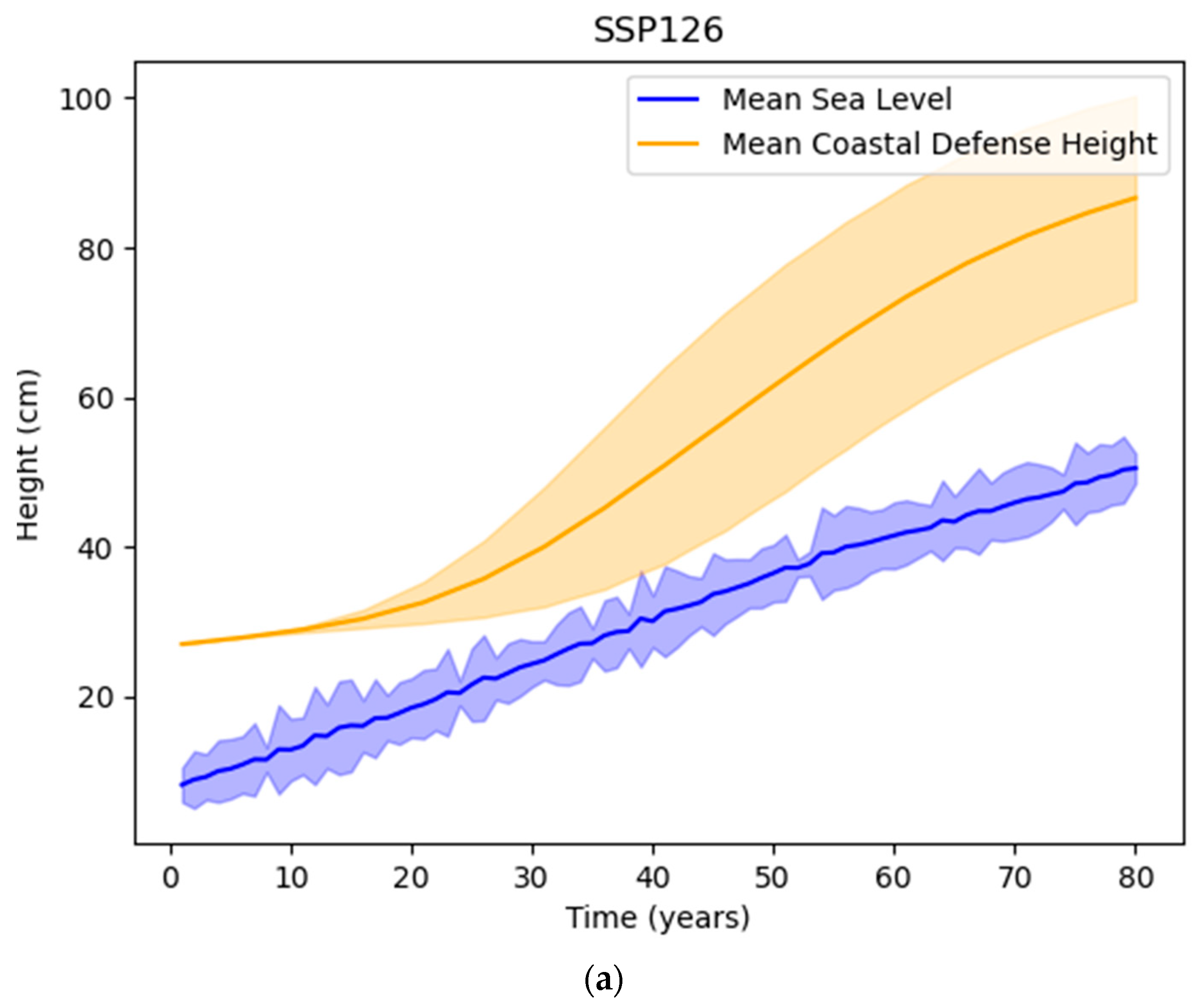
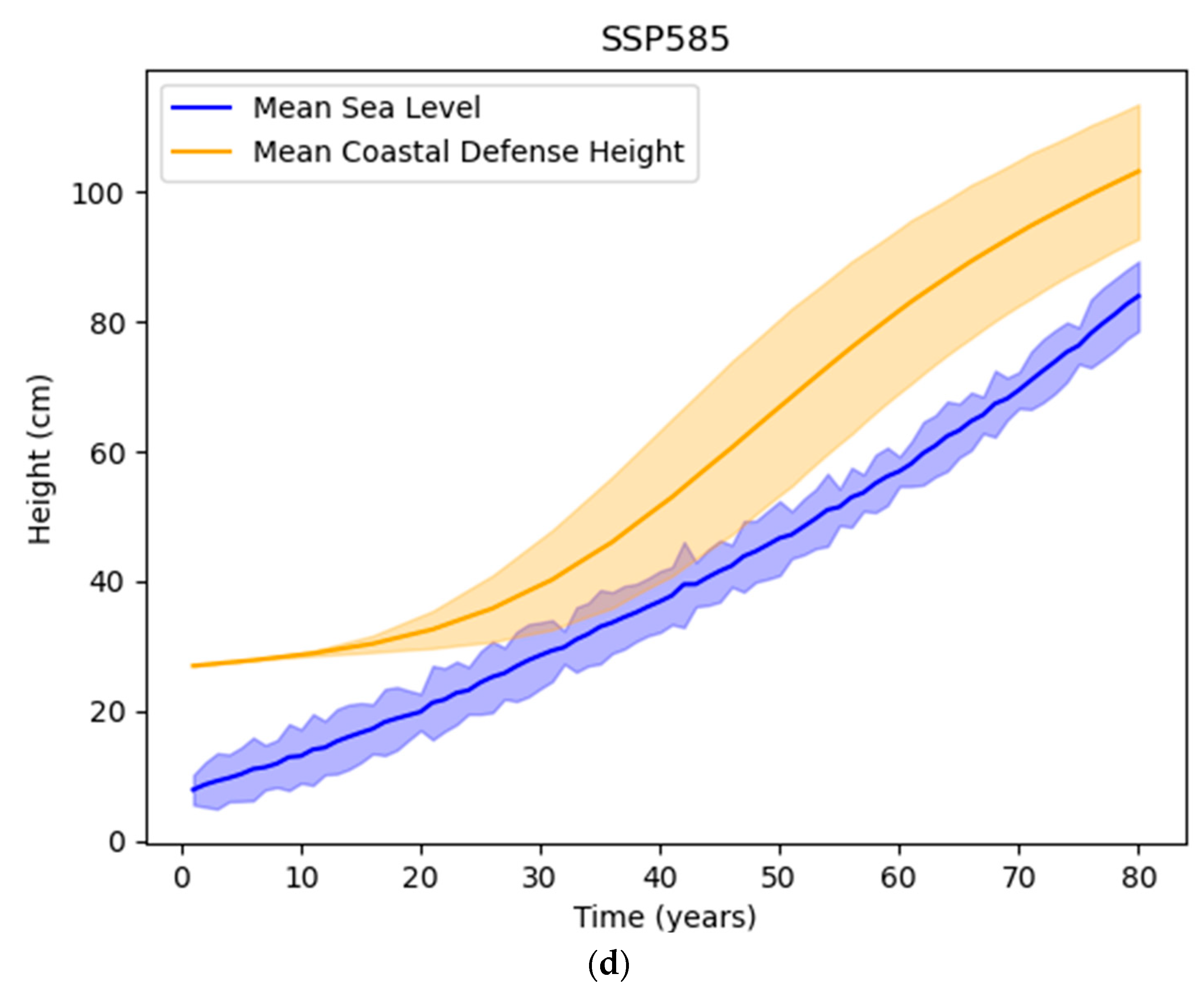
The agent is most successful at adapting to the SSP126 scenario. On average, damages are sustained from extreme events in the initial stages of the simulation. However, by the end of the simulation, coastal defenses are sufficiently developed to minimize damages from extreme sea-level events. In scenarios with more warming, i.e., SSP370 and SSP585, damages from extreme events are more evenly distributed throughout the simulation. Success parameters for these scenarios are shown in Table 5.
3.5. Effect of “Hedging”
In addition to reacting purely to expected sea-level rise, the planner can hedge against risks as a precautionary measure. Effectively, this means the planner prepares defenses corresponding to even higher sea levels than expected. We define a hedging factor fh, which changes the agent’s expected sea level H as per the expression:
For the “high-cost” scenario, we observe the following agent-averaged response curves for three different values of the hedging factor, as shown in Figure 12.
As observed, even in a scenario with high costs of coastal defense, the agent’s precautionary hedging leads to much more developed defenses due to higher investments. Due to this hedging, the agent does not start decreasing investments once an acceptable defense level is reached, heightening defenses to a much higher point than the sea level.
The success parameters in Table 6 show that precautionary defense heightening is slightly more effective from a pure damage avoidance perspective, with the city sustaining nearly zero damages from sea-level rise-related hazards. From a cost–benefit perspective, it is also seen that hedging against damages in this manner turns out to be much more inefficient. The expenses incurred by investments in coastal defense that hedge against possible risks far outweigh the damages avoided. In practice, this means that the precise costs of defense heightening and potential damages from flooding need to be known in order to determine the optimal level of investment [11,12]. Here, we have calculated the results for a hypothetical case. This framework can be applied to real-world cases to simulate trade-offs between different investments, hedging levels, and sea-level rise scenarios. It should also be noted that adaptation success is not significantly increased when the hedging factor h is increased from 1 to 2, as all of the agent’s available capital is already being utilized for heightening coastal defenses. Precautionary hedging is a trade-off between the efficiency of resources invested and a decrease in the risk of damages.
4. Discussion
The urban planner agent in our model is characterized by reactive behavior with a learning aspect, leading to the overall effect of the agent keeping pace with sea-level rise. Damages to the city from extreme sea-level rise and flood events are sustained primarily at the start of the simulation when defenses are not sufficiently heightened. In particular cases, extreme sea-level events occur earlier in the simulation, causing damages and spurring an agent response that decreases damages from similar (and even higher) extreme events later. However, this pattern is sensitive to the costs of heightening coastal defenses, and in the case of lower costs, earlier damages are also mitigated. When the agent’s expected damages in the next year decrease, adaptation investments decrease, leading to stagnation in the city’s coastal defenses.
The single-agent VIABLE-based model of the coastal city serves as an interactive tool that can be used to model adaptation responses across diverse scenarios in a user-friendly manner due to its being coded in NetLogo. However, from its concrete foundation of decision rules and dynamic adaptation action, it can also be further developed by extending these rules to multiple agents (as the VIABLE framework models multi-agent interactions) or implementing them in a spatially explicit environment.
5. Conclusions
The VIABLE model framework is successfully implemented for the case of a single-agent model of an urban planner of a coastal city managing adaptation actions in response to climate change-induced sea-level rise and related hazards.
We find that early extreme events have a priming effect that leads to more successful adaptation to later such events. This effect is borne out by similar real-world examples, which should be considered when planning adaptation policies. However, the timing of adaptation actions is also dependent on the costs involved.
We introduce three aspects of adaptation success that can be used to compare diverse scenarios in a quantifiable manner: the fraction of timesteps with zero damages sustained, total damages avoided, and the ratio of avoided damages to adaptation costs. This leverages the advantages of agent-based models to construct and analyze various possible futures of agent action. We apply these parameters to our sample scenarios and projected sea-level rise under different SSP scenarios.
With the addition of a system of precautionary hedging, the agent allocates much larger amounts of its resources to developing coastal defenses, and its adaptation actions show increased success. However, this leads to a worse outcome in terms of adaptation efficiency from a cost–benefit perspective, highlighting the trade-off involved in such measures. Nevertheless, it should be stressed that the costs involved are based purely on the potential damages avoided within the time horizon of the simulation, and the long-term effects of building coastal defenses should be incorporated into the cost–benefit analysis for adaptation planning.
Author Contributions
Conceptualization, S.S., D.V.K. and J.S.; formal analysis, S.S., D.V.K., L.M.B. and J.S.; funding acquisition, D.V.K., L.M.B. and J.S.; investigation, S.S., D.V.K., L.M.B. and J.S.; methodology, S.S. and D.V.K.; project administration, D.V.K., L.M.B. and J.S.; software, S.S.; supervision, D.V.K., L.M.B. and J.S.; visualization, S.S.; writing—original draft, S.S., D.V.K. and J.S.; writing—review and editing, S.S., D.V.K., L.M.B. and J.S. All authors have read and agreed to the published version of the manuscript.
Funding
This work was conducted and financed within the framework of the Helmholtz Institute for Climate Service Science (HICSS), a cooperation between Climate Service Center Germany (GERICS) and Universität Hamburg, Germany [Project “Modeling Urban Dynamics Affected by Climate Change for Coastal Spatial Planning and Management” (MUCCCS)].
Data Availability Statement
Parameters are contained within the article. The NetLogo Model code is included along with the article.
Acknowledgments
The authors are grateful for the support provided by members of GERICS and members of the CLICCS B3 project “Conflict and Cooperation at the Climate-Security Nexus”.
Conflicts of Interest
The authors declare no conflict of interest.
Appendix A
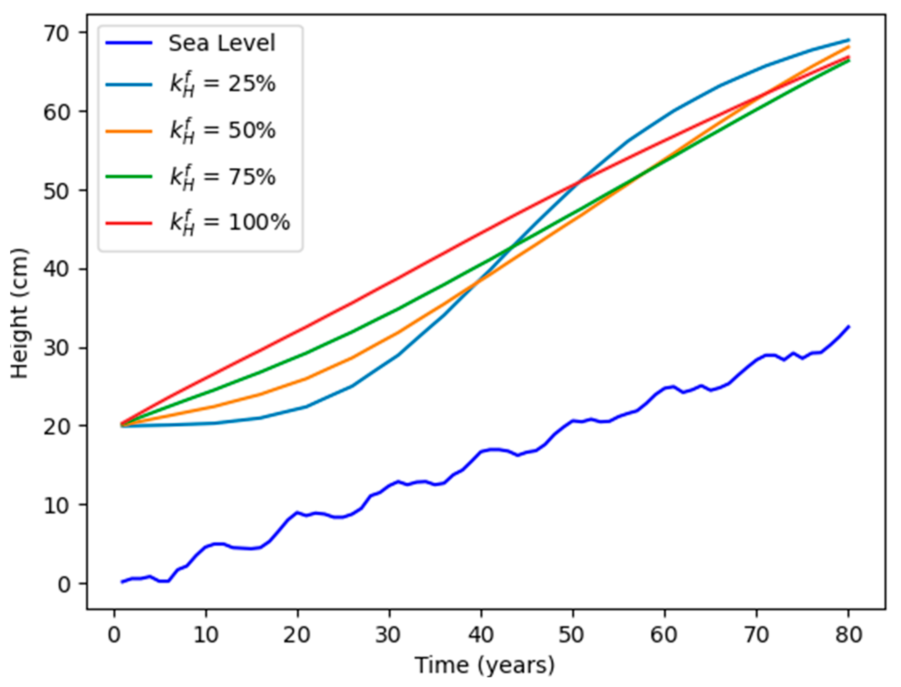
To investigate the effect of varying the fractional efficiency of coastal defense heightening on agent adaptation action, we carry out a sensitivity analysis for this parameter, taking values of 25%, 50%, 75%, and 100% (at 0% efficiency, the agent cannot invest in defense heightening at all and effectively cannot act). As described above, fractional efficiency represents inefficiencies in governance and adaptation plan implementation and is heavily system-dependent.
From the agent response curves in Figure A1, we observe that at 25% efficiency, the agent takes much longer to adapt to rising sea levels and overshoots the optimal defense height due to slower plan implementation. The speed of agent response increases with increasing efficiency until 100%, where the agent’s averaged response is completely linear, following the gradual sea-level rise.
Figure A1.
Averaged coastal defense height for varying values of fractional efficiency of coastal defense heightening.
Figure A1.
Averaged coastal defense height for varying values of fractional efficiency of coastal defense heightening.

Appendix B
At every timestep, the optimizing agent has to calculate the optimal value V*, which will represent its target. We have defined the value of the agent as follows:
where utility U and disutility W are given by:
where , and income obtained from the city Y = capital K, and is a parameter describing the relative importance of negative utility with respect to positive utility.
The damage function is taken as:
From the state dynamics equations, at the end of every timestep:
Substituting these in the damage function, the value equation becomes:
To obtain a linearly increasing function for d that starts rising after the value of excess height crosses a threshold value h0 > 0, we take it as a piecewise function defined as:
where hs > 0.
Taking , the value equation in terms of CH and CR becomes:
where θ is a step function defined as:
We make a few substitutions for brevity:
This reduces the value equation to:
With the constraint that .
In addition, whenever , the optimal total investment amount would be zero, so we can take as another constraint.
To find an analytical solution for V*, we introduce:
Defining the value equation in terms of these new parameters:
In this equation, when , the disutility term disappears, leaving value dependent decreasingly on , i.e., , so for maximizing, we impose the constraint that .
So, we have the following boundary constraints:
Staying within the domain bound at ,,, and (Figure A2), we can vary a parameter such that . Thus, keeping constant, we find that the minimum value of V is reached at , and increases towards the edges of the domain. Thus, we can infer that the maximum value of V is reached at the boundary of this domain. Applying this to both and , we can see that V is maximized when either or .
Figure A2.
Boundary constraints on and .

To find a solution analytically, we assume :
Since only the boundary conditions result in a maximization, either or holds true (in both cases, the other parameter is variable).
To maximize the above, we consider an auxiliary function f defined as:
where q > 0 and x lies between the bounds xmin and xmax. f(x) has an extremum point at x0 where:
Thus, the maximum value of f(x) is reached at xmin, xmax, or x0. The terms f(xmin), f(xmax), and f(x0) would have to be computed, and the corresponding value of x would therefore be the target value.
So, to maximize , we use the following algorithm:
- Since either or holds true, we first make these substitutions:
- We then compute , and , where:
- We conduct a similar substitution for the case, where :
- We now similarly compute , and , where:
- The values of and that correspond to the maximum value of out of the terms computed in Steps 2 and 4, are the target values and .
The above algorithm yields target values and , which are used to calculate C* and r* as follows:
Appendix B.1. Special Case for α and β
To take a more generalized scenario, we can prescribe that utility increases linearly and disutility changes at an arbitrary rate > 0, i.e., and .
We start with the value equation as computed earlier, this time substituting instead:
where β is an arbitrary positive value.
We take a similar auxiliary function:
As a result, the same algorithm is followed, with only the terms and calculated in Steps 2 and 4, respectively, being changed:
where and .
The rest of the algorithm remains unchanged.
References
- UNPD (United Nations, Department of Economic and Social Affairs, Population Division), World Urbanization Prospects: The 2018 Revision. The United Nations: New York. 2019. Available online: https://www.google.com/url?sa=t&rct=j&q=&esrc=s&source=web&cd=&ved=2ahUKEwjbhNCD9K2AAxVEyGEKHYD1A8YQFnoECBYQAQ&url=https%3A%2F%2Fpopulation.un.org%2Fwup%2Fpublications%2FFiles%2FWUP2018-Report.pdf&usg=AOvVaw33RksR7fLXlpPYrI7Q4Poq&opi=89978449 (accessed on 1 July 2023).
- Fox-Kemper, B.; Hewitt, H.T.; Xiao, C.; Aðalgeirsdóttir, G.; Drijfhout, S.S.; Edwards, T.L.; Golledge, N.R.; Hemer, M.; Kopp, R.E.; Krinner, G.; et al. Ocean, Cryosphere and Sea Level Change. In Climate Change 2021: The Physical Science Basis. Contribution of Working Group I to the Sixth Assessment Report of the Intergovernmental Panel on Climate Change; Masson-Delmotte, V., Zhai, P., Pirani, A., Connors, S.L., Péan, C., Berger, S., Caud, N., Chen, Y., Goldfarb, L., Gomis, M.I., et al., Eds.; Cambridge University Press: Cambridge, UK; New York, NY, USA,, 2021; pp. 1211–1362. [Google Scholar]
- Pörtner, H.-O.; Roberts, D.C.; Adams, H.; Adelekan, I.; Adler, C.; Adrian, R.; Aldunce, P.; Ali, E.; Begum, R.A.; Friedl, B.B.; et al. Climate Change 2022: Impacts, Adaptation and Vulnerability; Cambridge University Press: Cambridge, UK; New York, NY, USA,, 2022; pp. 37–118. [Google Scholar]
- Schelling, T.C. Dynamic models of segregation. J. Math. Sociol. 1971, 1, 143–186. [Google Scholar]
- Sakoda, J.M. The checkerboard model of social interaction. J. Math. Sociol. 1971, 1, 119–132. [Google Scholar]
- Yang, L.E.; Scheffran, J.; Süsser, D.; Dawson, R.; Chen, Y.D. Assessment of flood losses with household responses: Agent-based simulation in an urban catchment area. Environ. Model. Assess. 2018, 23, 369–388. [Google Scholar]
- Dawson, R.J.; Peppe, R.; Wang, M. An agent-based model for risk-based flood incident management. Nat. Hazards 2011, 59, 167–189. [Google Scholar]
- Taberna, A.; Filatova, T.; Roy, D.; Noll, B. Tracing resilience, social dynamics and behavioral change: A review of agent-based flood risk models. Socio-Environ. Syst. Model. 2020, 2, 17938. [Google Scholar]
- BenDor, T.K.; Scheffran, J. Agent-Based Modeling of Environmental Conflict and Cooperation; Taylor & Francis Group: Boca Raton, FL, USA, 2018; p. 333. [Google Scholar]
- Yang, L.E.; Hoffmann, P.; Scheffran, J.; Rühe, S.; Fischereit, J.; Gasser, I. An agent-based modeling framework for simulating human exposure to environmental stresses in urban areas. Urban Sci. 2018, 2, 36. [Google Scholar]
- Kind, J.M. Economically efficient flood protection standards for the Netherlands. J. Flood Risk Manag. 2014, 7, 103–117. [Google Scholar] [CrossRef]
- Vrijling, J.K.; van Hengel, W.; Houben, R.J. Acceptable risk as a basis for design. Reliab. Eng. Syst. Saf. 1998, 59, 141–150. [Google Scholar] [CrossRef]
- Jonkman, S.N.; Hillen, M.M.; Nicholls, R.J.; Kanning, W.; van Ledden, M. Costs of adapting coastal defences to sea-level rise—New estimates and their implications. J. Coast. Res. 2013, 29, 1212–1226. [Google Scholar]
- Kron, W.; Müller, O. Efficiency of flood protection measures: Selected examples. Water Policy 2019, 21, 449–467. [Google Scholar]
- Garner, G.; Hermans, T.H.J.; Kopp, R.; Slangen, A.; Edwards, T.; Levermann, A.; Nowicki, S.; Palmer, M.; Smith, C.J.; Fox-Kemper, B.; et al. IPCC AR6 WGI Sea Level Projections. Version 20210809. PO.DAAC, CA, USA. Available online: https://podaac.jpl.nasa.gov/announcements/2021-08-09-Sea-level-projections-from-the-IPCC-6th-Assessment-Report (accessed on 13 May 2022).
- Kopp, R.E.; Garner, G.G.; Hermans, T.H.J.; Jha, S.; Kumar, P.; Slangen, A.B.A.; Turilli, M.; Edwards, T.L.; Gregory, J.M.; Koubbe, G.; et al. The Framework for Assessing Changes To Sea-level (FACTS) v1.0-rc: A platform for characterizing parametric and structural uncertainty in future global, relative, and extreme sea-level change, EGUsphere [preprint]. Available online: https://podaac.jpl.nasa.gov/announcements/2021-08-09-Sea-level-projections-from-the-IPCC-6th-Assessment-Report (accessed on 13 May 2022).
- Jevrejeva, S.; Jackson, L.P.; Riva, R.E.M.; Grinsted, A.; Moore, J.C. Coastal sea level rise with warming above 2 °C Proc. Natl. Acad. Sci. USA 2016, 113, 13342–13347. [Google Scholar] [CrossRef] [PubMed]
Figure 1.
Shape of the damage function d(h) and the minimum threshold height h0.

Figure 2.
Comparison of agent investments in adaptation pathways over time.

Figure 3.
Comparison of averaged sea level with coastal defense height for the “high-cost” scenario (error bars represent one standard deviation).
Figure 3.
Comparison of averaged sea level with coastal defense height for the “high-cost” scenario (error bars represent one standard deviation).

Figure 4.
Comparison of averaged damages with coastal defense investment for the “high-cost” scenario (error bars represent one standard deviation).
Figure 4.
Comparison of averaged damages with coastal defense investment for the “high-cost” scenario (error bars represent one standard deviation).

Figure 5.
Comparison of averaged sea level with coastal defense height for the “low-cost” scenario.

Figure 6.
Comparison of averaged damages with coastal defense investment for the “low-cost” scenario.
Figure 6.
Comparison of averaged damages with coastal defense investment for the “low-cost” scenario.

Figure 7.
Agent response to early extreme sea-level events.

Figure 8.
Agent response to later extreme sea-level events.

Figure 9.
Projected sea-level rise under different SSP scenarios for the “Cuxhaven 2” tide gauge location [15,16].

Figure 10.
Comparison of averaged sea level with coastal defense height (high-cost coastal defenses) for SSP scenarios: (a) SSP126; (b) SSP245; (c) SSP370; and (d) SSP585.
Figure 10.
Comparison of averaged sea level with coastal defense height (high-cost coastal defenses) for SSP scenarios: (a) SSP126; (b) SSP245; (c) SSP370; and (d) SSP585.


Figure 11.
Comparison of averaged annual damages with annual coastal defense investments (high-cost coastal defenses) for SSP scenarios: (a) SSP126; (b) SSP245; (c) SSP370; and (d) SSP585.
Figure 11.
Comparison of averaged annual damages with annual coastal defense investments (high-cost coastal defenses) for SSP scenarios: (a) SSP126; (b) SSP245; (c) SSP370; and (d) SSP585.


Figure 12.
Comparison of averaged sea level with coastal defense height for: (a) ; (b) ; (c) .


Table 1.
Sea-level rise scenarios implemented in the model.
| Scenario Name | Scenario Description (Changes in Sea Level H in cm) |
|---|---|
| Gradual (deterministic) | H + 1 for five steps after every five timesteps |
| Gradual with extreme events (probabilistic) | H + 1 + x for five steps after every five timesteps, where x is a randomized value that has an increasing chance to be non-zero with time |
Table 2.
Model units and their equivalents.
| Model Units and Their Equivalents | |
| Timestep (time units) | Years |
| Height Units (for sea-level rise and coastal defense height) | Centimeters |
| Monetary Units | Millions euro (M €) |
| Area Units | Square kilometers |
Table 3.
Model Parameters and initial values of model variables.
| Model Parameters | |
| Adaptation rate α | 0.5 |
| Fractional investment efficiency into coastal defense development kHf | 0.5 |
| Investment efficiency into city relocation kRf | 0.1 |
| Defense depreciation rate | 0.05 cm/yr |
| Baseline percentage probability of extreme sea-level events at each timestep | 3.00 |
| Increase in percentage probability of extreme sea-level events per timestep | 0.01 |
| Initial Variable Values | |
| Coastal Area | 10 sq. km |
| Inland Area | 10 sq. km |
| Unit Income from the coastal territory | 20 M €/sq. km |
Table 4.
Adaptation success parameters for high-cost and low-cost scenarios.
| Scenario | ACD | ADA (%) | ACB (%) |
|---|---|---|---|
| High-cost | 1.00 | 97.07 | 69.78 |
| Low-cost | 1.00 | 97.12 | 201.63 |
Table 5.
Adaptation success parameters for different scenarios of sea-level rise.
| Scenario | ACD | ADA (%) | ACB (%) |
|---|---|---|---|
| SSP126 | 1.00 | 97.06 | 55.81 |
| SSP245 | 1.00 | 97.05 | 52.81 |
| SSP370 | 1.00 | 97.05 | 49.86 |
| SSP585 | 1.00 | 97.03 | 46.45 |
Table 6.
Adaptation success parameters for different values of hedging factor .
| Scenario | ACD | ADA (%) | ACB (%) |
|---|---|---|---|
| = 2 | 1.00 | 97.12 | 20.15 |
| = 1 | 1.00 | 97.12 | 32.87 |
| = 0.5 | 1.00 | 97.11 | 42.95 |
Disclaimer/Publisher’s Note: The statements, opinions and data contained in all publications are solely those of the individual author(s) and contributor(s) and not of MDPI and/or the editor(s). MDPI and/or the editor(s) disclaim responsibility for any injury to people or property resulting from any ideas, methods, instructions or products referred to in the content. |
© 2023 by the authors. Licensee MDPI, Basel, Switzerland. This article is an open access article distributed under the terms and conditions of the Creative Commons Attribution (CC BY) license (https://creativecommons.org/licenses/by/4.0/).
Share and Cite
MDPI and ACS Style
Sengupta, S.; Kovalevsky, D.V.; Bouwer, L.M.; Scheffran, J. Urban Planning of Coastal Adaptation under Sea-Level Rise: An Agent-Based Model in the VIABLE Framework. Urban Sci. 2023, 7, 79. https://doi.org/10.3390/urbansci7030079
AMA Style
Sengupta S, Kovalevsky DV, Bouwer LM, Scheffran J. Urban Planning of Coastal Adaptation under Sea-Level Rise: An Agent-Based Model in the VIABLE Framework. Urban Science. 2023; 7(3):79. https://doi.org/10.3390/urbansci7030079
Chicago/Turabian StyleSengupta, Shubhankar, Dmitry V. Kovalevsky, Laurens M. Bouwer, and Jürgen Scheffran. 2023. "Urban Planning of Coastal Adaptation under Sea-Level Rise: An Agent-Based Model in the VIABLE Framework" Urban Science 7, no. 3: 79. https://doi.org/10.3390/urbansci7030079