
A Numerical Method for Simulating Viscoelastic Plates Based on Fractional Order Model


1
School of Science, Yanshan University, Qinhuangdao 066004, China
2
Department of Mathematics, Taiyuan Normal University, Jinzhong 030600, China
3
Key Laboratory for Engineering & Computational Science, Shanxi Provincial Department of Education, Taiyuan Normal University, Jinzhong 030600, China
4
Institute of Advanced Forming and Intelligent Equipment, Taiyuan University of Technology, Taiyuan 030024, China
5
College of Science, North China University of Science and Technology, Tangshan 063000, China
*
Authors to whom correspondence should be addressed.
Fractal Fract. 2022, 6(3), 150; https://doi.org/10.3390/fractalfract6030150
Submission received: 30 January 2022
/
Revised: 7 March 2022
/
Accepted: 8 March 2022
/
Published: 10 March 2022
(This article belongs to the Special Issue Applications of Fractional Operator in Image Processing and Stability of Control Systems)
Abstract
:In this study, an efficacious method for solving viscoelastic dynamic plates in the time domain is proposed for the first time. The differential operator matrices of different orders of Bernstein polynomials algorithm are adopted to approximate the ternary displacement function. The approximate results are simulated by code. In addition, it is proved that the proposed method is feasible and effective through error analysis and mathematical examples. Finally, the effects of external load, side length of plate, thickness of plate and boundary condition on the dynamic response of square plate are studied. The numerical results illustrate that displacement and stress of the plate change with the change of various parameters. It is further verified that the Bernstein polynomials algorithm can be used as a powerful tool for numerical solution and dynamic analysis of viscoelastic plates.
1. Introduction
Plate and plate structure are widely used in many realms of mechanical, building and aerospace [1]. In addition, the plate is also a key component in aerospace engineering, which bears strong and sudden power including vibration. They are usually combined with viscoelastic materials to reduce the applied vibration and have the effect of damping [2]. In order to apply plate structure more widely in real life, many scholars are committed to the research of plate vibration. Early scholars analyzed the linear vibration of plates. Ziaee [3] used the Ritz method to study linear vibration of nanoplates. The effects of different parameters on polysilicon microplate were discussed. Cadou et al. [4] considered the linear vibration of the plate and testified availability of the method used for calculating eigenvalues of linear problems. Gradually, the research direction of some scholars began to change to nonlinear plate. Based on the semi-analytical method, Babahammou et al. [5] researched linear and nonlinear vibration of plates under the condition of full line or partial line support. Cho [6] proposed an algorithm for analyzing nonlinear vibration problems. The parameters of nonlinear free vibration characteristics of composite plates were discussed. Quan et al. [7] established the governing equation of sandwich plate vibration by using shear deformation theory and analyzed the nonlinear vibration of plate by Galerkin method and fourth-order Runge Kutta method. Although there have been a lot of research results, there are still problems in viscoelastic plates.
Viscoelastic materials have both elasticity and viscosity and are widely used for passive vibration isolation in engineering structures and applications owing to their light weight and high intensity. Therefore, it is essential to model viscoelastic materials properly [8,9]. In recent years, scholars have proposed various models to describe viscoelastic material. In order to simulate the elastic and viscous properties of materials at the same time, the fractional viscoelastic model is replaced by the classical viscoelastic model. The behavior of the system cannot only be appropriately described by fractional order model with less parameters but also fitted by fractional order operator [10]. Therefore, fractional order has a wide range of applications, especially in control systems. Using the multi-switch synchronization method, Pan et al. [11] considered the sliding-mode combinatorial synchronization of fractional-order chaotic systems under double random disturbances. Zhang et al. [12] introduced fractional order into sliding mode control of the system. The nonlinear term is estimated by using radial basis function neural network. Zhang et al. [13] provided a set of criteria for fractional order systems stability and verified the efficiency of controllers with numerical examples. With the development of viscoelastic material structure, some scholars gradually use fractional order to model viscoelastic plate. Rouzegar et al. [14] derived the governing equations of viscoelastic plate with Voigt viscoelastic model. The variation of amplitude and frequency of fractional viscoelastic plates under external excitation was given. Permoon et al. [15] discussed the natural frequency and characteristics of viscoelastic plate. Three constitutive models were compared by fitting a curve. Praharaj et al. [16] employed fractional damping derivative model to simulate plate structure. How the different orders of fractional order affect the vibration response of the plate was considered by combining the two methods to solve the differential equations. Ai et al. [17] established the finite element equations of stiffened plate by using fractional merchant model. The influences of altitude and overall arrangement on time-varying behavior of plates were analyzed.
The research on the numerical solution of viscoelastic plates is equivalent to the solution of fractional governing equation. In other words, numerical analysis of the viscoelastic plates not only needs to establish the material behavior equation but also an effective numerical method to approximate fractional governing dynamic equations. The common methods for solving the mentioned equations include Laplace transform [18], Fourier transform [19], Galerkin method [20], meshless method [21], multi-scale method [22] and variational iteration method [23]. Due to the large amount of calculation and difficulty to obtain the inverse transform, these methods are very difficult for obtaining solutions of this kind of equation directly in the time domain. However, plate differential governing equations take critical part in the wide application of engineering science. So, in recent years, polynomial approximation method has been widely used in solving fractional differential equations. Wang et al. [24] used shifted Legendre polynomials to approximate variable fractional differential equations. The dynamic response of viscoelastic pipe conveying fluid was analyzed. Hashim et al. [25] proposed shifted Chebyshev polynomials of the second kind to solve approximate solutions of time-delay variable fractional differential equations. Cao et al. [26] studied a significant method based on fractional rheological model to solve viscoelastic column problems. The fractional differential equation was solved by shifted Chebyshev wavelet function. Compared with the above polynomials, Bernstein polynomials have the advantages of simple structure and perfect properties. Therefore, it is widely used in solving differential equations and practical engineering applications [27]. More and more scholars use Bernstein polynomials to solve all kinds of differential equations. By using Bernstein polynomials, Khan et al. [28] obtained the calculation results of fractional constitutive equation. In this method, the coupled system is transformed into algebraic equations by operator matrix. Heydari et al. [29] proposed Bernstein polynomials to approximate advection diffusion reaction equation with fractal fractional derivative. Chen et al. [30] utilized Bernstein polynomials to solve a series of variable fractional order differential equations. Different Bernstein polynomials matrices were derived and used to transform initial equations into discrete nonlinear equations. However, the above studies are limited to solving fractional differential equations using Bernstein polynomials. Few studies directly solve such equations in time domain and analyze the dynamic behavior combined with three-dimensional plates.
For these reasons, it is necessary to combine the fractional order model with a new calculation method to settle the above problem. Therefore, the Bernstein polynomials algorithm is proposed to numerically simulate differential equations of the plate and analyze the effects of parameters on the numerical solutions of the displacement and stress. This algorithm has good applicability to calculate the fractional governing equation of three-dimensional plates in the time domain. It is also fit for dynamic analysis of viscoelastic plates. In addition, this technology will supply a new approach for the numerical study of viscoelastic plates.
The paper is structured as follows: The preliminary knowledge of Caputo derivative is recommended in Section 2. Section 3 presents the governing equation of three-dimensional viscoelastic plate by using the fractional constitutive model. Section 4 derives the matrices of Bernstein polynomials. Demand problem is expressed by various orders differential operator matrices. In Section 5, the availability of the proposed algorithm is verified by two methods. Section 6 discusses displacements of plate under various conditions. Finally, conclusions of this paper are obtained in Section 7.
2. Preliminaries
Next, several properties and mathematical preliminaries of fractional calculus are given, which will be applied in the following sections.
Definition 1.
The fractional Caputo derivative of order α is defined as [31]
where is Caputo fractional differential operator, is fractional order, f is integrable and continuous on , is Gamma function and has .
Based on the Caputo derivative, we have
3. Governing Equation of Fractional Viscoelastic Plate
In this part, a fractional viscoelastic plate shown in Figure 1 with sides of a and b, thickness of h is studied. This rectangular plate is fixedly supported on four sides. The motion equation of the plate is as follows [33]
where is mass density, is constant damping for the fractional derivative element model, is biharmonic operator, is flexural stiffness, E is Young’s modulus, v is the Poisson’s ratio, is the Airy stress function and is transverse force excitation.
From the above formulas, the governing equation of fractional viscoelastic plate is expressed as [34,35]
The boundary conditions of plate with four fixed edges are
4. Numerical Algorithm for Bernstein Polynomials
In this section, Bernstein polynomials algorithm is introduced to approximate unknown functions. The governing equations are transformed from differential operator matrices into algebraic equations.
4.1. Bernstein Polynomials
Definition 2.
The definition of Bernstein polynomials of degree m in is [36]
The following formula is written as
Expand the binomial to obtain the following formula
For expanding the scope of x, Bernstein polynomials in is written as
where R is any positive integer.
A matrix consisted by Bernstein polynomials is
where
4.2. Function Approximation
For any continuous function with one variable, it can be expressed by Bernstein polynomials as
where .
The inner product is calculated as
where .
Similarly, the function of two variables can be approximated as
where .
The function of t is approximated as
where .
4.3. Differential Operator Matrix of Bernstein Polynomials
4.3.1. Integer Differential Operator Matrix
Definition 3.
satisfaction is the 1th operator matrix of Bernstein polynomials. The derivation procedure is as follows
where and .
4.3.2. Fractional Differential Operator Matrix
Definition 5.
satisfaction is the αth operator matrix of Bernstein polynomials.
The partial differential term in Equation (5) is formulated as
4.4. Discretizationdiscretization Governing Equation
The governing equation can be expressed by various orders differential operator matrices as
The boundary conditions are converted into
Configure variable as discrete variable . Matrices W and N areis gained by MATLAB software. Thus, the initial equation is solved.
5. Error Analysis and Mathematical Example
For the sake of proving accuracy and effectiveness of the mentioned Bernstein polynomials algorithm, the following error analysis is carried out.
5.1. Error Bound
Theorem 1.
If and is the best approximation of . , ,
Proof.
The Taylor expansion of is
where
Because is the best approximation of , there is
where and .
Therefore, Theorem 1 is proved. Similarly, when , it can be proved in the same way based on Bernstein polynomials. The results show that the proposed algorithm is precise and efficacious for approximating unknown functions of three variables. □
5.2. Mathematical Example
The accuracy of the algorithm is verified by a mathematical example. It is represented by the following equation. The parameters in the mathematical example can be any values and have no realistic significance. The specific equation is as follows
The boundary conditions are
where , , and .
The exact solution is
Substituting exact solution into Equation (35), mathematical equation is derived as
The Bernstein polynomials algorithm with the number of items is used to solve the proposed mathematical example. The numerical solution is . The absolute error is
Figure 2a,b is the analytical and numerical solutions, respectively, at . It can be seen that numerical solution and analytical solution are remarkably unanimous. Figure 2c shows absolute error and its minimum order of magnitude can reach . It can be proved that this method is high accuracy and its availability for simulating governing equations of fractional viscoelastic plates.
6. Numerical Analysis
The equation of the fractional quadrilateral clamped square plate is numerically analyzed. The plate displacement under external load is being investigated. The effect of different side lengths of the square plate on plate displacement is analyzed. Dynamic behavior of fractional plate with three boundary conditions is studied. In addition, the effect of thickness of the plate on the stress is also studied. In all subsequent studies, the time parameter is always considered as . Table 1 shows geometric characteristics of viscoelastic plate materials in dynamic analysis.
6.1. Influence of Different Simple Harmonic Loads on Plate Displacement
When taking the parameters in Table 1 for research, different simple harmonic loads are exerted to clamped square plate. Its form is . Figure 3 is the dynamic response of a square plate. It can be found that the displacement of plate is symmetric at and reaches the maximum at the center point. With an increase in simple harmonic load coefficient , the displacement of square plate also increases. Furthermore, when the load condition is , the results of Table 2 are obtained through fixed width . Displacement also increases with load and is symmetrical at the midpoint of the length.
6.2. Influence of Side 0 of the Plate on Plate Displacement
In this part, the influences of different side lengths of square plates on plate displacement are studied. Figure 4 is the change of displacement with side length of the plate under load .
It can be seen that the displacement of the square plate increases with side length. This is consistent with the results of Reference [40], but this paper can use the proposed algorithm to solve the problem directly in the time domain. In Reference [40], a weak formal equation was constructed based on Hamilton’s principle and a four node rectangular plate element was used to discretize the region. When different external loads were used, the vibration response of the laminated plate was studied by refined plate theory finite element approach. The results indicate that Bernstein polynomials algorithm is an efficacious tool for solving fractional differential equations of three-dimensional plates. Displacement solution obtained by this algorithm has high accuracy.
6.3. Influence of Boundary Conditions on Plate Displacement
Figure 5 is about the influence of three boundary conditions on displacement of viscoelastic plates. CCCC, SSCC and SSSS denote completely simply supported plate, simply supported clamped plate and completely clamped plate in proper order. The expressions for the three of them are
As summarized from the figures, the square plate with the minimum constraints has the largest displacement, and the displacement of plate decreases with increase in constraints. This is consistent with the findings in Reference [40]. In this paper, the three-dimensional diagram is used to more intuitively show the change of displacement with constraints. This means that the displacement of the plate can be reduced by increasing the constraint of boundary conditions. Therefore, the proposed algorithm provides a theoretical basis for study of vibration analysis of viscoelastic plates.
6.4. Influence of Plate Thickness on Stress
The variation of stress with plate thickness will be analyzed. The expression for stress is
The stress distribution of the viscoelastic plate under external load is shown in Figure 6. The displacement of the plate will increase by the thickness of the plate. The conclusion is consistent with Reference [2]. By using the generalized multi-axial Maxwell model and Hamilton’s principle, they obtained the viscoelastic constitutive equation and proposed an effective equal geometric analysis formula for solving the nonlinear vibration problem of the viscoelastic plate. This verifies correctness of the numerical results. Therefore, the proposed algorithm is suitable for solving and studying stress problems of viscoelastic plates.
7. Conclusions
A new method for calculating fractional differential equations is presented in this paper. The differential operator matrices of Bernstein polynomials are used to approximate the displacement function directly in the time domain. The governing equations are transformed into algebraic equations for the solution. Error analysis and numerical results prove the correctness and effectiveness of the mentioned algorithm. In addition, the dynamic response of the three-dimensional viscoelastic plate is analyzed.
1. The displacement of viscoelastic plate is gained directly in the time domain by Bernstein polynomials algorithm. The unknown function is approximated by the operator matrix form of the mentioned polynomials.
2. The displacement of plate increases with the increase in the simple harmonic load coefficient and side length of square plate. The smaller the boundary condition constraints, the larger the viscoelastic plate displacement.
3. The effect of the plate thickness on stress is discussed. As the thickness of the plate increases, the stress value also increases.
4. The proposed algorithm can be applied to more complex differential governing equations, such as variable fractional viscoelastic plates and shells.
Author Contributions
Conceptualization, S.J. and J.X.; methodology, S.J.; software, S.J. and J.Q.; formal analysis, Y.C.; data curation, Y.C.; writing—original draft preparation, S.J.; project administration, Y.C.; funding acquisition, J.X. All authors have read and agreed to the published version of the manuscript.
Funding
This work is supported by the National Natural Science Foundation of China (Grant No.52005360) and Technological innovation Programs of Higher Education Institution in Shanxi (2021L403).
Conflicts of Interest
The authors declare that they have no known competing financial interests or personal relationships that could have appeared to influence the work reported in this paper.
References
- Zhang, D.P.; Lei, Y.J.; Shen, Z.B. Semi-analytical solution for vibration of nonlocal piezoelectric Kirchhoff plates resting on viscoelastic foundation. J. Appl. Comput. Mech. 2018, 4, 202–205. [Google Scholar] [CrossRef]
- Shafei, E.; Faroughi, S.; Rabczuk, T. Nonlinear transient vibration of viscoelastic plates: A NURBS-based isogeometric HSDT approach. Comput. Math. Appl. 2018, 84, 1–15. [Google Scholar] [CrossRef]
- Ziaee, S. Linear free vibration of micro-/nano-plates with cut-out in thermal environment via modified couple stress theory and Ritz method. Ain Shams Eng. J. 2018, 9, 2373–2381. [Google Scholar] [CrossRef]
- Cadou, J.M.; Ounis, H.; Boutyour, E.H.; Potier-Ferry, M. Asymptotic numerical method and Padé approximants for eigenvalue.Application in linear vibration of plates and shells. Mech. Res. Commun. 2020, 106, 103538. [Google Scholar] [CrossRef]
- Babahammou, A.; Benamar, R. Linear and nonlinear vibrations of isotropic rectangular plates resting on full or partial line supports. Mater Today Proc. 2022, in press. [Google Scholar] [CrossRef]
- Cho, J.R. Nonlinear free vibration of functionally graded CNT-reinforced composite plates. Compos. Struct. 2022, 281, 115101. [Google Scholar] [CrossRef]
- Quan, T.Q.; Ha, D.T.T.; Duc, N.D. Analytical solutions for nonlinear vibration of porous functionally graded sandwich plate subjected to blast loading. Thin Wall Struct. 2022, 170, 108606. [Google Scholar] [CrossRef]
- Datta, N.; Praharaj, R.K. Dynamic response of fractionally damped viscoelastic plates subjected to a moving point load. J. Vib. Acoust. 2020, 142, 041002. [Google Scholar] [CrossRef]
- Katsikadelis, J.T.; Babouskos, N.G. Post-buckling analysis of viscoelastic plates with fractional derivative models. Eng. Anal. Bound. Elem. 2010, 34, 1038–1048. [Google Scholar] [CrossRef]
- Fan, W.P.; Jiang, X.Y.; Qi, H.T. Parameter estimation for the generalized fractional element network Zener model based on the Bayesian method. Physica A 2015, 427, 40–49. [Google Scholar] [CrossRef]
- Pan, W.Q.; Li, T.Z.; Wang, Y. The multi-switching sliding mode combination synchronization of fractional order non-identical chaotic system with stochastic disturbances and unknown parameters. Fractal Fract. 2022, 6, 102. [Google Scholar] [CrossRef]
- Zhang, X.F.; Lin, C.; Chen, Y.Q.; Boutat, D. A unified framework of stability theorems for LTI fractional order systems with 0 < α < 2. IEEE Trans. Circuits Syst. II Express Briefs 2020, 67, 3237–3241. [Google Scholar] [CrossRef]
- Zhang, X.F.; Huang, W.K. Adaptive neural network sliding mode control for nonlinear singular fractional order systems with mismatched uncertainties. Fractal Fract. 2020, 4, 50. [Google Scholar] [CrossRef]
- Rouzegar, J.; Vazirzadeh, M.; Heydari, M.H. A fractional viscoelastic model for vibrational analysis of thin plate excited by supports movement. Mech. Res. Commun. 2020, 110, 103618. [Google Scholar] [CrossRef]
- Permoon, M.R.; Farsadi, T. Free vibration of three-layer sandwich plate with viscoelastic core modelled with fractional theory. Mech. Res. Commun. 2021, 116, 103766. [Google Scholar] [CrossRef]
- Praharaj, R.K.; Datta, N. On the transient response of plates on fractionally damped viscoelastic foundation. Comput. Appl. Math. 2020, 39, 256. [Google Scholar] [CrossRef]
- Ai, Z.Y.; Jiang, Y.H.; Zhao, Y.Z.; Mu, J.J. Time-dependent performance of ribbed plates on multi-layered fractional viscoelastic cross-anisotropic saturated soils. Eng. Anal. Bound. Elem. 2022, 137, 1–15. [Google Scholar] [CrossRef]
- Sene, N.; Fall, A.N. Homotopy perturbation ρ-Laplace transform method and its application to the fractional diffusion equation and the fractional diffusion-reaction equation. Fractal Fract. 2019, 3, 14. [Google Scholar] [CrossRef] [Green Version]
- Zainal, N.H.; Kiliçman, A. Solving fractional partial differential equations with corrected Fourier series method. Abstr. Appl. Anal. 2014, 2014, 958931. [Google Scholar] [CrossRef] [Green Version]
- Qiu, W.L.; Xu, D.; Chen, H.F.; Guo, J. An alternating direction implicit Galerkin finite element method for the distributed-order time-fractional mobile–immobile equation in two dimensions. Comput. Math. Appl. 2020, 80, 3156–3172. [Google Scholar] [CrossRef]
- Nikan, O.; Avazzadeh, Z.; Machado, J.A.T. Numerical study of the nonlinear anomalous reaction–subdiffusion process arising in the electroanalytical chemistry. J. Comput. Sci.-Neth. 2021, 53, 101394. [Google Scholar] [CrossRef]
- Mohamadi, A.; Shahgholi, M.; Ghasemi, F.A. Free vibration and stability of an axially moving thin circular cylindrical shell using multiple scales method. Meccanica 2019, 54, 2227–2246. [Google Scholar] [CrossRef]
- Cherif, M.H.; Ziane, D. Variational iteration method combined with new transform to solve fractional partial differential equations. Univ. J. Math. Appl. 2018, 1, 113–120. [Google Scholar] [CrossRef]
- Wang, Y.H.; Chen, Y.M. Dynamic analysis of the viscoelastic pipeline conveying fluid with an improved variable fractional order model based on shifted Legendre polynomials. Fractal Fract. 2019, 3, 52. [Google Scholar] [CrossRef] [Green Version]
- Hashim, I.; Sharadga, M.; Syam, M.I.; Al-Refai, M. A reliable approach for solving delay fractional differential equations. Fractal Fract. 2022, 6, 124. [Google Scholar] [CrossRef]
- Cao, J.W.; Chen, Y.M.; Wang, Y.H.; Zhang, H. Numerical analysis of nonlinear variable fractional viscoelastic arch based on shifted Legendre polynomials. Math. Method Appl. Sci. 2021, 11, 8798–8813. [Google Scholar] [CrossRef]
- Wang, J.S.; Liu, L.Q.; Chen, Y.M.; Ke, X.H. Numerical solution for fractional partial differential equation with Bernstein polynomials. J. Electron. Sci. Technol. 2014, 12, 331–338. [Google Scholar] [CrossRef]
- Khan, H.; Alipour, M.; Jafari, H.; Khan, R.A. Approximate analytical solution of a coupled system of fractional partial differential equations by Bernstein polynomials. Int. J. Appl. Comput. Math. 2016, 2, 85–96. [Google Scholar] [CrossRef] [Green Version]
- Heydari, M.H.; Avazzadeh, A.; Yang, Y. Numerical treatment of the space-time fractal-fractional model of nonlinear advection-diffusion-reaction equation through the Bernstein polynomials. Fractals 2020, 28, 2040001. [Google Scholar] [CrossRef]
- Chen, Y.M.; Liu, L.Q.; Liu, D.Y.; Boutat, D. Numerical study of a class of variable order nonlinear fractional differential equation in terms of Bernstein polynomials. Ain Shams Eng. J. 2018, 9, 1235–1241. [Google Scholar] [CrossRef] [Green Version]
- Yi, M.X.; Huang, J. Wavelet operational matrix method for solving fractional differential equations with variable coefficients. Appl. Math. Comput. 2014, 230, 383–394. [Google Scholar] [CrossRef]
- Chen, Y.M.; Sun, Y.N.; Liu, L.Q. Numerical solution of fractional partial differential equations with variable coefficients using generalized fractional-order Legendre functions. Appl. Math. Comput. 2014, 244, 847–858. [Google Scholar] [CrossRef]
- Malara, M.; Spanos, P.D. Nonlinear random vibrations of plates endowed with fractional derivative elements. Probabilist. Eng. Mech. 2018, 54, 2–8. [Google Scholar] [CrossRef]
- Timosenko, S.P. Theory of Plates and Shells; McGraw-Hill: New York, NY, USA, 1964. [Google Scholar]
- Jiang, Q.; Zhou, Z.D.; Yang, F.P. The method of fundamental solutions for two-dimensional elasticity problems based on the Airy stress function. Eng. Anal. Bound. Elem. 2021, 130, 220–237. [Google Scholar] [CrossRef]
- Khataybeh, S.N.; Hashim, I.; Alshbool, M. Solving directly third-order ODEs using operational matrices of Bernstein polynomials method with applications to fluid flow equations. J. King Saud Univ. Sci. 2019, 31, 822–826. [Google Scholar] [CrossRef]
- Kiasat, M.S.; Zamani, H.A.; Aghdam, M.M. On the transient response of viscoelastic beams and plates on viscoelastic medium. Int. J. Mech. Sci. 2014, 83, 133–145. [Google Scholar] [CrossRef]
- Wang, J.; Xu, T.Z.; Wang, G.W. Numerical algorithm for time-fractional Sawada-Kotera equation and Ito equation with Bernstein polynomials. Appl. Math. Comput. 2018, 338, 1–11. [Google Scholar] [CrossRef]
- Kadkhoda, N. A numerical approach for solving variable order differential equations using Bernstein polynomials. Alex. Eng. J. 2020, 59, 3041–3047. [Google Scholar] [CrossRef]
- Rouzegar, J.; Davoudi, M. Forced vibration of smart laminated viscoelastic plates by RPT finite element approach. Acta Mech. Sin. 2020, 36, 933–949. [Google Scholar] [CrossRef]
Figure 1.
The geometric figure of four sides fixed support viscoelastic plate.

Figure 2.
The mathematical example results for (a) analytical solution, (b) numerical solution and (c) absolute error at different points.
Figure 2.
The mathematical example results for (a) analytical solution, (b) numerical solution and (c) absolute error at different points.

Figure 3.
Plate displacements under three simple harmonic loads for (a) . (b) . (c) .

Figure 4.
Displacements under external load at different side lengths for (a) . (b) . (c) .
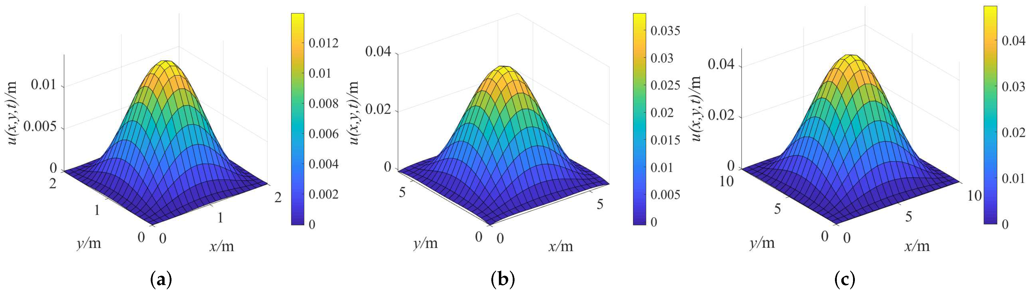
Figure 5.
Displacements of the plate under external load at different boundary conditions for (a) CCCC. (b) SSCC. (c) SSSS.
Figure 5.
Displacements of the plate under external load at different boundary conditions for (a) CCCC. (b) SSCC. (c) SSSS.
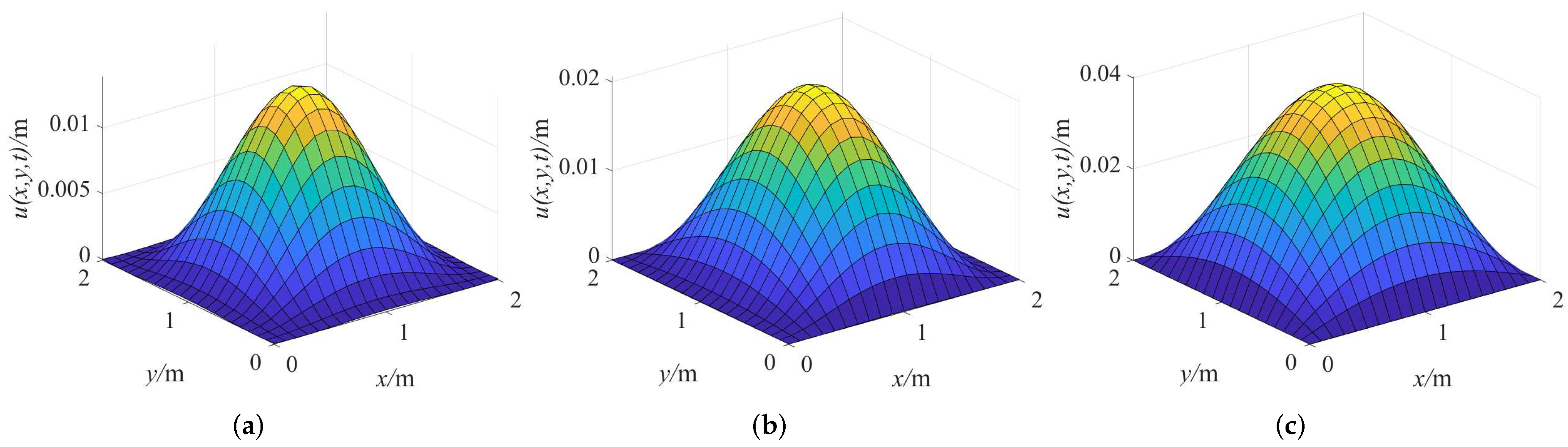
Figure 6.
Stress of the plate under external load at different plate thickness for (a) . (b) . (c) .
Figure 6.
Stress of the plate under external load at different plate thickness for (a) . (b) . (c) .


Table 1.
Geometric properties of viscoelastic plate materials [8].
Table 1.
Geometric properties of viscoelastic plate materials [8].
| Physical Quantity | Symbol | Value | Dimension |
|---|---|---|---|
| Fractional order | 0.75 | 1 | |
| Length | a | 2 | |
| Width | b | 2 | |
| Thickness | h | 0.02 | |
| Density of the plate | 7850 | ||
| Poisson’s ratio | v | 0.3 | 1 |
| Young’s modulus | E | ||
| Damping coefficient | 1 |
Table 2.
Displacement numerical solutions under simple harmonic loads.
| 0 | 0 | ||||
| 0 | 0 | ||||
| 0 | 0 |
Publisher’s Note: MDPI stays neutral with regard to jurisdictional claims in published maps and institutional affiliations. |
© 2022 by the authors. Licensee MDPI, Basel, Switzerland. This article is an open access article distributed under the terms and conditions of the Creative Commons Attribution (CC BY) license (https://creativecommons.org/licenses/by/4.0/).
Share and Cite
MDPI and ACS Style
Jin, S.; Xie, J.; Qu, J.; Chen, Y. A Numerical Method for Simulating Viscoelastic Plates Based on Fractional Order Model. Fractal Fract. 2022, 6, 150. https://doi.org/10.3390/fractalfract6030150
AMA Style
Jin S, Xie J, Qu J, Chen Y. A Numerical Method for Simulating Viscoelastic Plates Based on Fractional Order Model. Fractal and Fractional. 2022; 6(3):150. https://doi.org/10.3390/fractalfract6030150
Chicago/Turabian StyleJin, Suhua, Jiaquan Xie, Jingguo Qu, and Yiming Chen. 2022. "A Numerical Method for Simulating Viscoelastic Plates Based on Fractional Order Model" Fractal and Fractional 6, no. 3: 150. https://doi.org/10.3390/fractalfract6030150