Mapping Maize Planting Densities Using Unmanned Aerial Vehicles, Multispectral Remote Sensing, and Deep Learning Technology

Abstract

Maize is a globally important cereal and fodder crop. Accurate monitoring of maize planting densities is vital for informed decision-making by agricultural managers. Compared to traditional manual methods for collecting crop trait parameters, approaches using unmanned aerial vehicle (UAV) remote sensing can enhance the efficiency, minimize personnel costs and biases, and, more importantly, rapidly provide density maps of maize fields. This study involved the following steps: (1) Two UAV remote sensing-based methods were developed for monitoring maize planting densities. These methods are based on (a) ultrahigh-definition imagery combined with object detection (UHDI-OD) and (b) multispectral remote sensing combined with machine learning (Multi-ML) for the monitoring of maize planting densities. (2) The maize planting density measurements, UAV ultrahigh-definition imagery, and multispectral imagery collection were implemented at a maize breeding trial site. Experimental testing and validation were conducted using the proposed maize planting density monitoring methods. (3) An in-depth analysis of the applicability and limitations of both methods was conducted to explore the advantages and disadvantages of the two estimation models. The study revealed the following findings: (1) UHDI-OD can provide highly accurate estimation results for maize densities (R² = 0.99, RMSE = 0.09 plants/m²). (2) Multi-ML provides accurate maize density estimation results by combining remote sensing vegetation indices (VIs) and gray-level co-occurrence matrix (GLCM) texture features (R² = 0.76, RMSE = 0.67 plants/m²). (3) UHDI-OD exhibits a high sensitivity to image resolution, making it unsuitable for use with UAV remote sensing images with pixel sizes greater than 2 cm. In contrast, Multi-ML is insensitive to image resolution and the model accuracy gradually decreases as the resolution decreases.

1. Introduction

Maize is one of the most widely cultivated cereal crops worldwide [1,2] and is extensively applied in human food, livestock feed, and fuel production [3]. The accurate detection of maize occurrences and the monitoring of its planting densities during the growth process are crucial, especially considering that early maize densities are a major factor that influences yields [4,5]. This study provides essential information for farm management, early breeding decisions, improving seedling emergence rates, and timely replanting [6].

Compared to traditional manual data collection methods, the use of unmanned aerial vehicles (UAVs) has increased efficiency, reduced personnel costs, and simplified the complexity of data collection [7,8]. In recent years, UAV applications for agricultural monitoring have rapidly developed. UAV-based monitoring offers highly flexible opportunities in terms of the temporal, spectral, and spatial resolutions, enabling more precise observations and analyses of crop growth and timely adjustments to management practices [9,10,11]. Moreover, UAVs equipped with various cameras, such as RGB digital and multispectral cameras, enable the rapid and accurate acquisition of crop growth information in the field [12,13,14]. Over the past two decades, researchers have explored UAV methods to replace the time-consuming manual extraction of crop trait information, which has achieved many successful outcomes [15].

Researchers use UAVs to efficiently capture high-resolution digital images of crops at the field scale and extract trait information by analyzing the crop texture features. This includes areas such as disease detection [16,17] and phenological predictions [18], among others, that are crucial for optimizing field management practices and predicting yields [19,20,21]. Current research has applied these methods in estimating the number of crops, including maize [4,6,22], wheat [23], rice [24], peanuts [25], and potatoes [26]. The success of these methods is primarily attributed to the development of deep learning technologies, which can automatically learn different features from images or datasets [27,28,29] and can effectively handle images with complex backgrounds that are captured by UAVs [30,31,32,33]. Especially in terms of the estimations of maize quantities, Liu et al. [34] used you only look once (YOLO) v3 to estimate the maize plant counts with a precision of 96.99%. Gao et al. [35] fine-tuned the Mask Region-convolutional neural network (R-CNN) model for automatic maize identification, achieving an average precision (AP) @ 0.5 intersection over union (IOU) of 0.729 and an average recall (AR)@ 0.5IOU of 0.837. Xu et al. [36], Xiao et al. [22], and others used the YOLOv5 model to estimate the maize plant counts from UAV digital images. Lucas et al. [37] proposed a CNN-based deep learning method for maize plant counting, with a precision of 85.6% and a recall of 90.5%. Vong et al. [38] developed an image processing workflow based on the U-Net deep learning model for maize segmentation and quantity estimation, with the highest counting accuracy occurring at R² = 0.95. While these methods achieve high accuracy, deep neural network models require substantial computational resources and large datasets for training [39,40,41,42]. Additionally, due to the small size of maize plants, low flight altitudes are necessary, resulting in slow data acquisition, poor real-time performance, and low efficiency. In practical applications, high-resolution digital image acquisition for maize plants when using UAVs is challenging.

The use of multispectral sensors and vegetation indices (VIs) in assessing plant growth status has achieved significant success in areas such as coverage [43,44], biomass [45,46,47], leaf area index (LAI) [48], nitrogen [49] and chlorophyll content [50]. However, its applications in estimating plant quantities and densities are relatively limited. The successful plant growth assessments using the VIs from multispectral sensors provide valuable insights for further exploration in this field. For instance, Sankaran et al. [51] used multispectral sensors and VIs to assess the emergence and spring survival rates of wheat by using UAV-obtained data. By using machine learning regression methods, Bikram et al. [52] estimated wheat quantities using spectral and morphological information that was extracted from multispectral images. Wilke et al. [53] evaluated wheat plant densities using UAV multispectral data and regression models. The application of multispectral data for estimating plant quantities and densities is still evolving, mainly due to the lower resolution of multispectral sensors compared to digital sensors, which lack the high resolution needed to accurately determine the geometric shapes of seedlings. However, multispectral imaging has the advantage of allowing the computation of VIs, which can be used in developing multivariate regression models for estimating plant traits [54].

At present, there is limited clarity regarding the suitability of ultrahigh-definition digital images and multispectral data for extracting maize planting density information through UAV-based remote sensing. Factors such as image resolution, spectral resolution, method selection (such as object detection or statistical regression), and their impact on results and mapping, have not been thoroughly understood. Therefore, there is a need for a more comprehensive comparison and evaluation of their practical application in this context.

The main tasks of this study are as follows: (1) Develop two UAV remote sensing-based methods for monitoring maize planting densities. These methods are based on ultrahigh-definition imagery combined with object detection (UHDI-OD) and multispectral remote sensing combined with machine learning (Multi-ML) for monitoring maize planting densities. (2) In addition, the maize planting densities were measured at a maize breeding trial site and UAV ultrahigh-definition imagery and multispectral imagery were collected. Experimental testing and validation were conducted using the proposed maize planting density monitoring methods. (3) Conduct in-depth analysis and investigation of the applicability and limitations of both methods. The advantages and disadvantages of the two estimation models were analyzed and discussed.

This study aimed to answer the following questions:

(1)

How can the maize planting densities be estimated by combining ultrahigh-definition RGB digital cameras, UAVs, and object detection models?

(2)

How can multispectral remote sensing sensors, UAVs, and machine learning techniques be integrated to estimate maize planting densities?

(3)

What are the advantages, disadvantages, and applicable scenarios for (a) UHDI-OD and (b) Multi-ML in estimations of maize planting densities?

2. Datasets

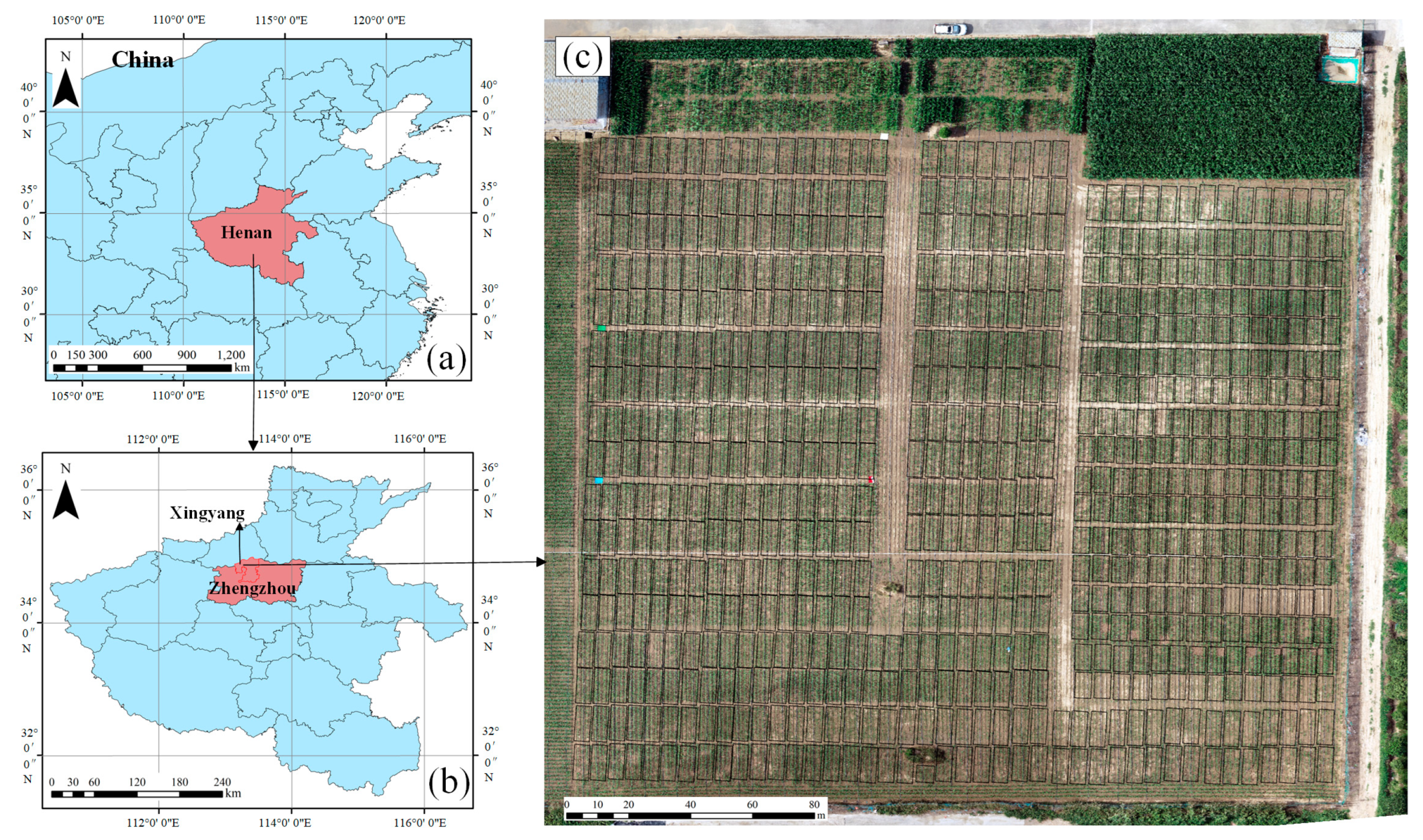
2.1. Study Area

The study area is located in Xingyang city, Henan Province, China (Figure 1a,b), with geographical coordinates ranging from 34°36′ to 34°59′ N and from 113°7′ to 113°30′ E. Xingyang city has a warm temperate continental monsoon climate, with average annual temperatures ranging from 12 to 16 °C. The experimental site is a maize breeding field (Figure 1c) and the experiment involved the UAV image collection of maize materials, conducted on 5 July 2023. The maize plants in the study area were in the V4 growth and development stages during the experiment.

2.2. UAV Data Collection

This study used a DJI Phantom 4 RTK (DJI Technology Co., Ltd., Shenzhen, China) and a Phantom 4 multispectral UAV as the image acquisition platforms to capture canopy images of maize in the experimental field. Considering the endurance of small UAVs, image resolution, and the safety of UAV flight heights, this study sets the flight height of the Phantom 4 RTK to 25 m and the flight height of the Phantom 4 Multispectral UAV to 20 m. DJI Terra software V4.0.1 version (DJI, Shenzhen) was employed for UAV image stitching. All UAV images were imported into DJI Terra software and both the digital and multispectral images were stitched based on the UAV and camera parameter settings.

The Phantom 4 RTK is equipped with an RGB digital camera with an effective pixel count of 20 million. The Phantom 4 Multispectral UAV is equipped with six sensors, one for visible light imaging (RGB sensor) and five for multispectral imaging (monochrome sensors). The multispectral images cover five bands, namely red (R), green (G), blue (B), red-edge, and near-infrared (NIR) regions. Each monochrome sensor has an effective pixel count of 2.08 million.

2.3. Maize Planting Density Measurements

The maize planting densities were calculated by dividing the number of maize plants within each plot by the corresponding measured area of that plot. The number of maize plants in each plot was obtained through manual counting, while the area of each plot was determined through on-site measurements of the geographic dimensions of the experimental area. This method ensures accurate information on both the number of maize plants and the corresponding area for each plot, thereby enabling the calculation of reliable and accurate maize planting densities. The average density of 790 measured planting plots is 6.64 plants/m², with a standard deviation of 1.28 plants/m², a maximum value of 9.45 plants/m², and a minimum value of 0 plants/m².

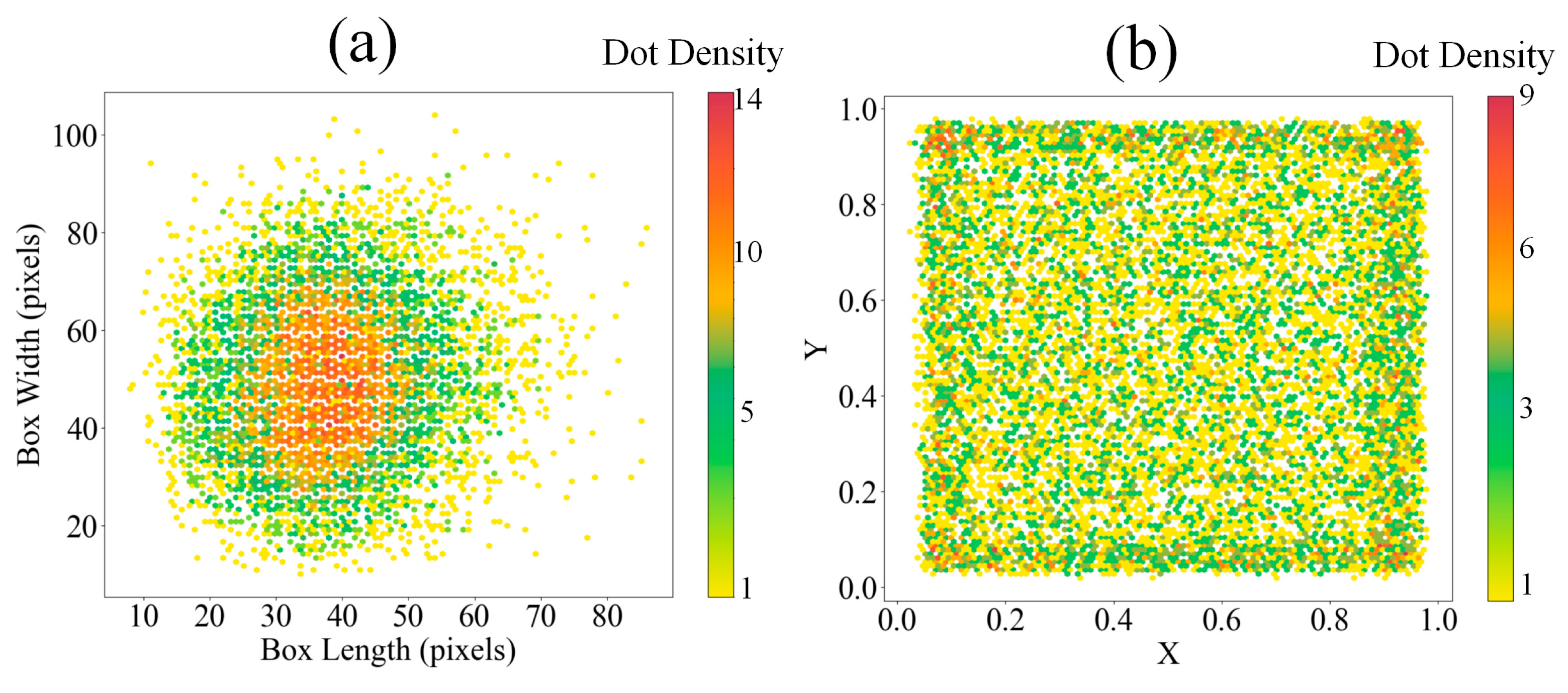
2.4. Maize Position Distribution

This study produced an orthomosaic by stitching together overlapping aerial images of the study area. This orthomosaic was subsequently divided into smaller, uniform patches, each covering an area of 256 × 256 pixels. These patches were annotated using LabelImg to create label files for object detection training. Images that did not represent the study area were excluded, leaving 807 images that met the requirements. A total of 14,272 maize plants were annotated within these images. The dataset was partitioned into training, validation, and test sets at a ratio of 6:2:2. Figure 2 illustrates the dimensions and spatial relationships of the bounding boxes outlining maize objects within this dataset. The “maize objects” denote complete maize plants delineated by bounding boxes in object detection. Generally, the maize objects in the images have dimensions smaller than 90 pixels, concentrated within a range of 25–45 pixels. Moreover, the relative positions of maize objects across the images demonstrate a relatively uniform distribution.

3. Methods

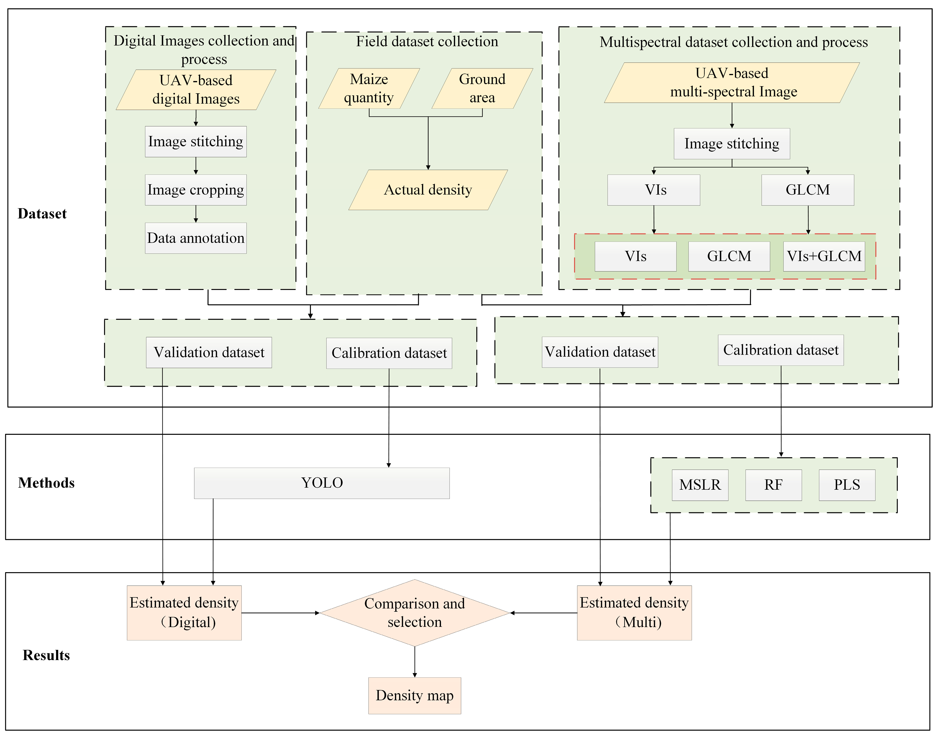
3.1. Methodology Framework

The main objective of this study is to propose and use two methods, UHDI-OD and Multi-ML, for accurately estimating planting density based on the high-resolution characteristics of data captured using RGB digital cameras and the multi-band characteristics of data captured using multispectral cameras. This study conducted a comprehensive analysis and study on the applicability and limitations of these two approaches. The technical workflow is shown in Figure 3 and the research work is divided into the following four primary tasks:

(1)

Data collection: This study used two UAVs equipped with an RGB digital camera and multispectral sensor to capture maize images in the field. These images were stitched together to generate a digital orthophoto mosaic of the entire area. The field data, including the number of maize plants and the size of the planting area, were obtained through field measurements to calculate the maize planting densities.

(2)

Digital image processing and density estimation: This study cropped and annotated the digital orthophoto mosaic and the annotated data into the YOLO object detection model for training. The goal was to find the most suitable model, obtain optimal maize detection results, and, consequently, estimate the planting densities.

(3)

Multispectral data processing and density estimation: This study extracted the VIs and the gray-level co-occurrence matrix (GLCM) texture features from the multispectral data. These features were combined and used in regression models (e.g., multiple linear stepwise regression (MLSR), random forest (RF), and partial least squares regression (PLS) to estimate the planting densities.

(4)

Comparison and selection of methods: This study comprehensively compared the advantages and disadvantages of the two methods and selected the most suitable model for mapping to accomplish the monitoring of the maize planting densities.

3.2. Proposed UHDI-OD Method for Extracting Planting Densities

3.2.1. Object Detection

YOLO is an end-to-end real-time object detection algorithm that was originally proposed by Joseph Redmon in 2016 [55]. Unlike traditional object detection methods, YOLO predicts an entire image in a single forward pass, providing advantages in terms of speed and real-time processing. In this study, the YOLO model was selected as the framework for maize recognition, as it enables object detection in images to acquire maize location information.

Different versions of YOLO [56,57] (such as YOLOv3, YOLOv5, and YOLOv8) have undergone improvements and optimizations that enhance detection performance and accuracy while supporting various application scenarios. Each version of the model has variants of different scales; for example, YOLOv8 includes five versions, ranging from YOLOv8n to YOLOv8s, YOLOv8m, YOLOv8l to YOLOv8x, with each version gradually increasing in model size. The improvement in performance and accuracy in each version is achieved by increasing the numbers of layers and parameters. This model not only considers its efficient real-time object detection capabilities, but also allows the selection of an appropriate version based on specific requirements, balancing model size and performance.

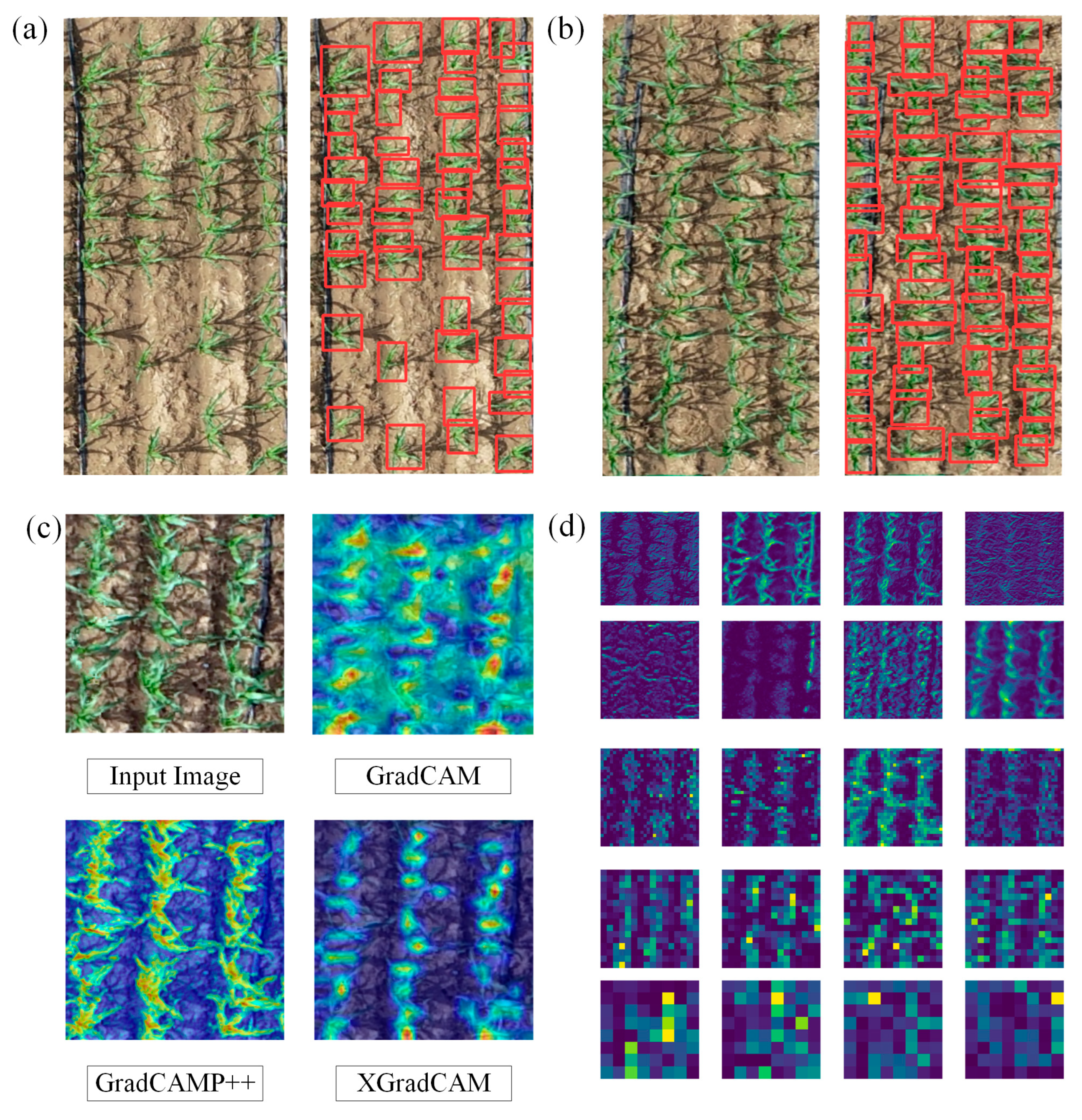
3.2.2. Visualization Methods

Gradient-weighted class activation mapping (Grad-CAM) [58] is a crucial technique for visualizing decisions made by deep neural networks (DNNs). Its principle is based on gradient information and the gradient weights of the last convolutional layer are captured to map these weights back to the input image, thereby generating a heatmap that intuitively displays the model’s focus areas on the input image. Grad-CAM++ [59] is an extension of Grad-CAM that enhances the spatial resolution and stability of heatmaps by introducing additional regularization terms. XGrad-CAM [60] is a further improvement of Grad-CAM, a CNN visualization method based on Axiom, which improves the robustness and interpretability of the heatmap.

This study uses and compares these three heatmap visualization methods, which not only visually demonstrate the key focus areas of the model on maize images, but also aid in understanding the decision-making process of the model, thereby enhancing the interpretability and explainability of deep learning models.

3.2.3. Planting Density Calculations Based on Object Detection

The maize quantity in each plot was precisely identified using object detection algorithms. The obtained quantity was then divided by the measured area of the corresponding plot to calculate the statistical value of the maize planting density. This method relies on ultrahigh-definition digital images to obtain accurate information about the maize planting densities, as calculated through the ratios of maize quantities to plot areas.

3.3. Proposed Multi-ML Method for Extracting Planting Densities

3.3.1. Vegetation Indices

Table 1. Spectral indices.

Name	Calculation	Reference
R	DN values of R band
G	DN values of G band
B	DN values of B band
Red-Edge	DN values of Red-Edge band
NIR	DN values of NIR band
NDVI	(NIR − R)/(NIR + R)	[61]
OSAVI	1.16 (NIR − R)/(NIR + R + 0.16)	[62]
LCI	(NIR − Red-Edge)/(NIR + R)	[63]
GNDVI	(NIR − G)/(NIR + G)	[64]
NDRE	(NIR − Red-Edge)/(NIR + Red-Edge)	[65]

shows commonly used VIs, most of which are constructed based on the reflectance characteristics of vegetation in the red, green, blue, and near-infrared channels. These spectral VIs use mathematical operations to enhance the vegetation information and establish empirical relationships between the maize planting densities and VIs.

3.3.2. Gray-Level Co-Occurrence Matrix

GLCM is an effective tool for describing the texture features in digital images. By analyzing the spatial relationships among the grayscale levels of the pixels in an image, the GLCM captures the texture variations among different regions in the image. The GLCM provides a reliable method used, in this study, to quantify the frequency and spatial distribution of different texture features in maize images. Based on the GLCM, this study can extract several important statistical features [66]. These features play a crucial role in obtaining a deeper understanding of the texture structure of an image, as detailed in

Table 2. Textural features of the GLCM.

Abbreviation	Name	Formula
Mea	Mean	${\displaystyle \sum _{i=1}^N} {\displaystyle \sum _{j=1}^N} i·P(i,j)$
Var	Variance	${\displaystyle \sum _{i=1}^N} {\displaystyle \sum _{j=1}^N} (i-{\mu }_i{)}^2·P(i,j)$
Hom	Homogeneity	${\displaystyle \sum _{i=0}^{N-1}} {\displaystyle \sum _{j=0}^{N-1}} \frac{P(i,j)}{1+{\left(i-j\right)}^2}$
Con	Contrast	${\displaystyle \sum _{i=0}^{N-1}} {\displaystyle \sum _{j=0}^{N-1}} {\left(i-j\right)}^{2}P(i,j)$
Dis	Dissimilarity	${\displaystyle \sum _{i=0}^{N-1}} {\displaystyle \sum _{j=0}^{N-1}} P(i,j)x|i-j|$
Ent	Entropy	$\sqrt{{\displaystyle \sum _{i=0}^{N-1}} {\displaystyle \sum _{j=0}^{N-1}} P(i,j{)}^2}$
ASM	Angular Second Moment	${\displaystyle \sum _{i=0}^{N-1}} {\displaystyle \sum _{j=0}^{N-1}} P(i,j{)}^2$
Cor	Correlation	${\displaystyle \sum _{i=0}^{N-1}} {\displaystyle \sum _{j=0}^{N-1}} \frac{(i-{\mu }_i)(j-{\mu }_j)P(i,j)}{\sqrt{({\sigma }_i)({\sigma }_j)}}$

Note: P(i,j) represents the position of an element in the GLCM, and μ represents the average of all gray-level values in the image area. μ_i and μ_j represent the average texture values in the x and y directions, respectively, while σ_i and σ_j represent the standard deviations in the x and y directions, respectively.

.

3.3.3. Statistical Regression

MLSR is a statistical method used to construct predictive models that explain the relationships between multiple independent variables and a dependent variable. It works through an iterative process by gradually adding or removing independent variables to optimize the model’s predictive accuracy and explanatory power. At each step, all possible combinations of the independent variables are considered and the optimal combination is selected to update the model. The advantage of multiple linear stepwise regression is its ability to handle multiple independent variables and to select the combination that best explains the dependent variable, while adapting the model’s complexity. However, this approach has several drawbacks, such as the potential for overfitting, high computational costs, and the possibility of overlooking important independent variables. To overcome these issues, researchers can explore regularization methods, cross-validation techniques, more efficient computational methods, or parallel computing techniques to speed up the calculations.

RF is a powerful ensemble learning method that produces predictions by building multiple decision trees and averaging their outputs. Each decision tree is independently trained on a randomly selected subset of features, which allows the model to handle a large number of features and complex relationships. The RF has a high tolerance for outliers and missing values, giving it an advantage in dealing with real-world data. However, its disadvantage lies in its lower interpretability, which makes it challenging to understand how each decision tree makes predictions. Additionally, the random forest algorithm may perform poorly when dealing with extreme values or outliers since the model’s training process may not sufficiently consider these situations.

PLS is an effective multivariate statistical analysis method. It addresses the issue of multicollinearity between variables by simultaneously projecting independent and dependent variables in a common direction. This regression modeling method is suitable for cases where the number of sample points is less than the number of independent variables and it retains all the original independent variables in the final model. Partial least squares regression models are easy to interpret and the regression coefficients for each independent variable are more interpretable. However, these methods have strict data requirements and need standardized data. Nonetheless, partial least squares regression may have limitations when dealing with complex data.

3.4. Accuracy Evaluation

3.4.1. Object Detection Evaluation

The evaluation metrics for the object detection results can be categorized into performance evaluations and complexity evaluations. Performance evaluation metrics include precision, recall, and mean average precision (mAP). Complexity evaluation metrics include the model size and floating-point operations (FLOPs). FLOPs represent the number of floating-point calculations performed during the inference process of the model.

The precision is the ratio of the number of correctly predicted positive samples to the total samples that were predicted as positive by the model and reflects the model’s classification accuracy. The recall measures the ratio of the number of correctly predicted positive samples to the total number of actual positive samples. The AP is the integral of the precision and recall, and the mAP is the average of the AP values across all classes and reflects the overall performance of the model in object detection and classification. The specific formulas for the calculations are as follows:

$$Precision=\frac{TP}{TP+FP}$$

(1)

$$Recall=\frac{TP}{TP+FN}$$

(2)

where TP represents true-positive (correctly predicted positive samples), FP represents false-positive (incorrectly predicted positive samples), and FN represents false-negative (incorrectly predicted negative samples).

$$AP={\int }_0^{1}Precision\left(Recall\right)dR$$

(3)

$$mAP=\frac{{\sum }_{i=1}^n{AP}_i}{n}$$

(4)

3.4.2. Planting Density Evaluation

For the regression methods used in this study, the coefficient of determination (R²) and root mean square error (RMSE) values were employed to assess the accuracy metrics of the models and methods presented in this paper.

$$R^2=1-\frac{{\sum }_{i=1}^n{(y_i-x_i)}^2}{{\sum }_{i=1}^n{(y_i-\overline{y})}^2}$$

(5)

$$\mathrm{R}\mathrm{M}\mathrm{S}\mathrm{E}=\sqrt{\frac{{\sum }_{i=1}^n{(x_i-y_i)}^2}{n}}$$

(6)

where x_i and y_i represent the estimated and observed sample values, respectively; ŷ represents the estimated mean; and n is the number of samples. Mathematically, for the same set of sample data, if the model yields a higher R² and a lower RMSE, it is generally considered that the model has greater accuracy.

4. Results

4.1. Maize Detection Based on Ultrahigh-Definition Digital Images

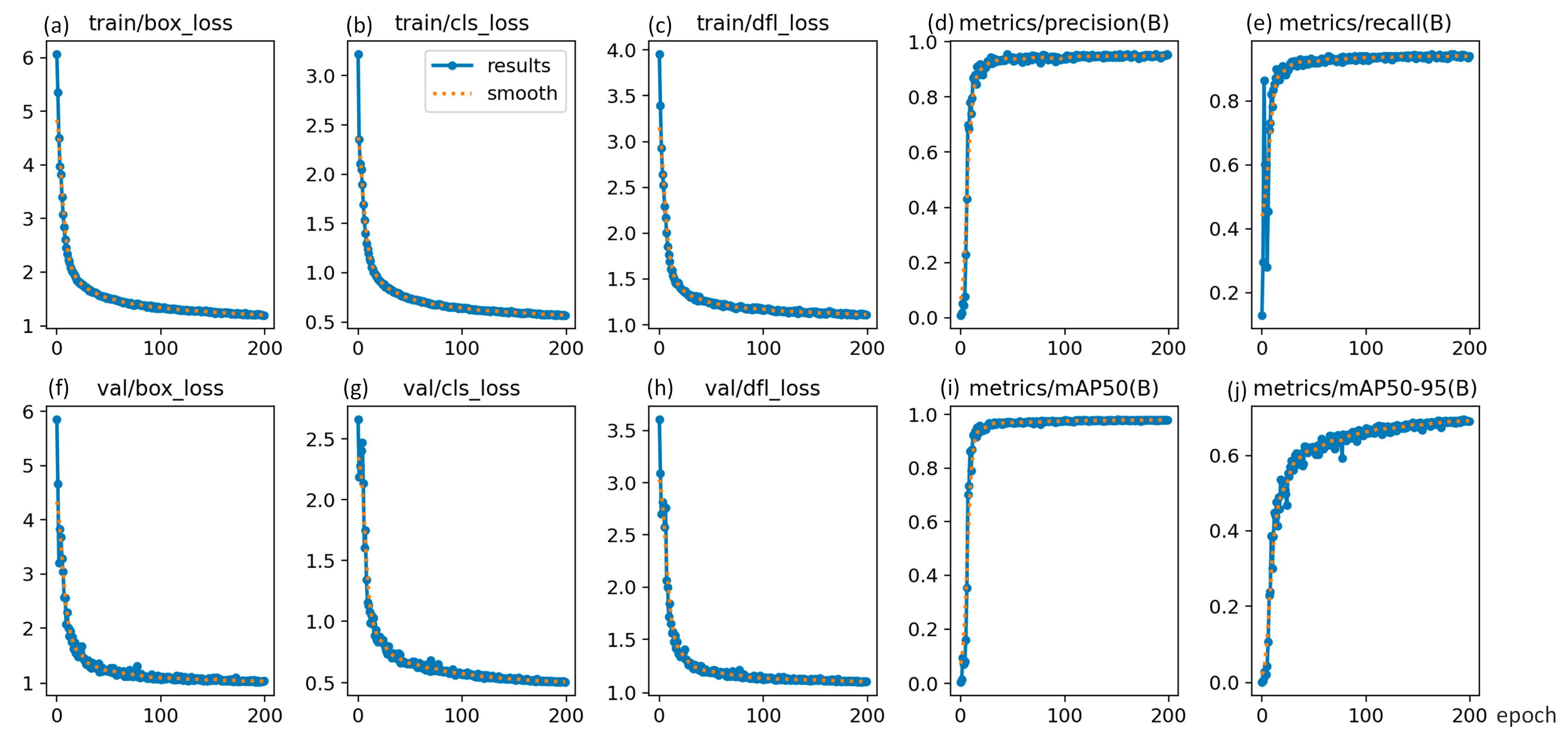
4.1.1. Object Detection Training and Recognition Results

In Figure 4, this study presents the training results curve for the optimal object detection model, YOLOv8n, that was trained for a total of 200 epochs. During the initial 100 epochs, we observed a rapid decrease in the bounding box loss (Box Loss), as shown in Figure 4a,f; the classification loss (Cls loss), shown in Figure 4b,g; and the dynamic feature learning loss (DFL Loss), shown in Figure 4c,h. Subsequently, after 100 epochs, these loss functions gradually stabilized. Additionally, improvements in precision (Figure 4d), recall (Figure 4e), mAP@50 (Figure 4i), and mAP@50-95 (Figure 4j) were evident in the first 20 epochs, which were followed by stable states.

Figure 5a,b show the identification results for those areas with different maize planting densities. It is evident that YOLOv8n demonstrates high accuracy and reliability in maize recognition and can be used to effectively handle images with varying planting densities. Figure 5c,d show the feature visualization and heatmaps of the recognition process. Feature visualization provides an intuitive understanding of how the maize features change through different modules during processing, allowing insights into the internal processing flow and decision-making mechanisms of the model.

This study conducted a comprehensive performance comparison between different versions of the YOLOv8 models and other YOLO-series models, and the results are presented in

Table 3. Comparison of the experimental results of each model.

Model	Precision (%)	Recall (%)	mAP@50 (%)	mAP@50-95 (%)	Param (M)	FLOPs (GFLOPS)
YOLOv8n	94.8	94.5	98.3	73.4	3.0	8.1
YOLOv8s	95.2	94.1	98.2	73.9	11.1	28.4
YOLOv8m	95.1	94.5	98.2	73.7	25.8	78.7
YOLOv8l	94.9	94.8	98.3	74.0	43.6	164.8
YOLOv8x	95.0	94.8	98.3	73.5	68.1	257.4
YOLOv3-tiny	93.9	94.4	97.9	72.4	12.1	18.9
YOLOv5n	94.9	94.3	98.2	73.0	1.7	4.1
YOLOv6n	94.5	93.8	98.2	73.3	4.2	11.8

. Except for the slightly lower accuracy in YOLOv3-tiny, the precisions of the other models are very similar. By comprehensively considering various metrics, this study chooses YOLOv8n as the maize target recognition model.

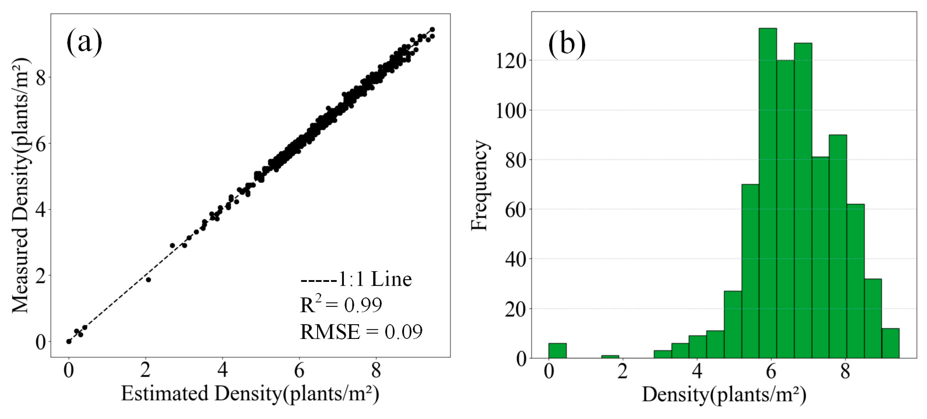
4.1.2. UHDI-OD Estimation Results for Planting Densities

This study used the trained YOLOv8n model to estimate the maize planting densities in 790 plots. The results are shown in Figure 6a. The results show highly accurate estimations, demonstrating a strong positive correlation between the model estimates and the actual observations, with R² = 0.99 and RMSE = 0.09 plants/m². Figure 6b shows the distribution of the maize planting densities, revealing that the majority of plots had densities ranging between 5 and 8.5 plants/m².

4.2. Maize Density Estimations Based on Multispectral Data

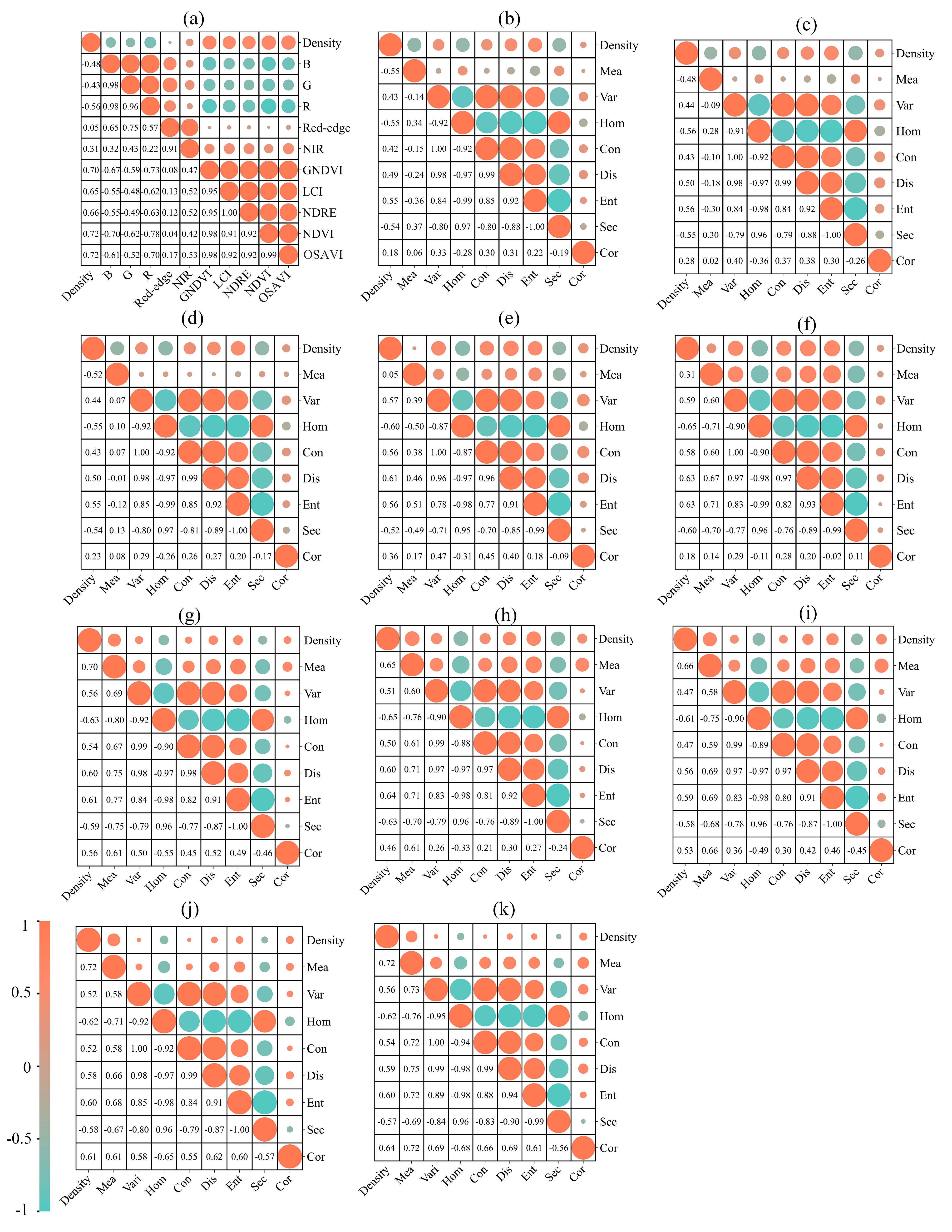
4.2.1. Correlation Analysis

For the multispectral data, this study conducted a correlation analysis among the maize planting densities, common VIs, and texture features that were obtained using the GLCM with the R, G, B, Red-edge, and NIR bands (Figure 7). The results of the correlation analysis revealed strong correlations among the maize planting densities and various VIs (e.g., GNDV, LCI, NDRE, NDVI, and OSAVI), while the correlations with the original five bands (e.g., R, G, B, Red-edge, and NIR) were relatively weak. However, after GLCM processing, the correlations of the original five bands with the planting densities increased significantly. For example, the correlation coefficient of the red edge band increased from 0.05 (Figure 7a) to 0.61 (Figure 7e). The various VIs (e.g., GNDV, LCI, NDRE, NDVI, and OSAVE) undergo GLCM processing, but their correlation coefficient with planting density is not enhanced; instead, most of the correlations are weakened (Figure 7g–k).

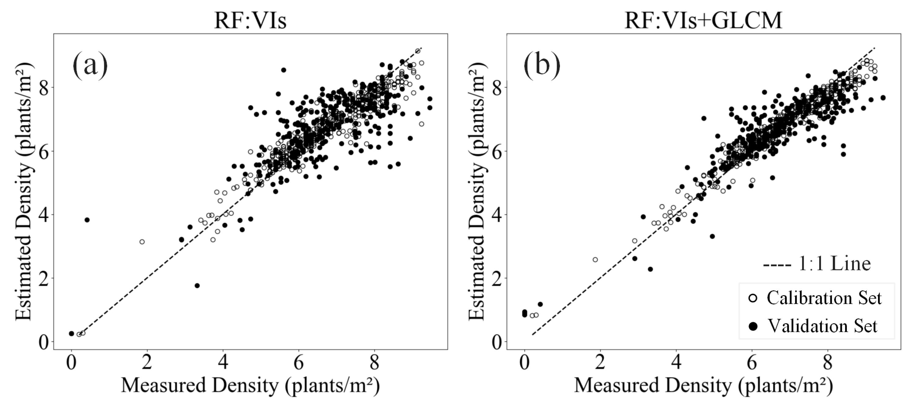
4.2.2. Multi-ML Estimations of Planting Densities

The results of estimating the maize planting densities using MSLR, RF, and PLS are presented in

Table 4. Results of planting density estimations.

Dataset	Methods	Calibration		Validation
		R2	RMSE (Plants/m2)	R2	RMSE (Plants/m2)
VIs	MSLR	0.50	0.86	0.55	0.92
	RF	0.89	0.39	0.59	0.87
	PLS	0.52	0.84	0.58	0.89
GLCM	MSLR	0.56	0.80	0.62	0.84
	RF	0.94	0.29	0.72	0.72
	PLS	0.69	0.67	0.74	0.70
VIs + GLCM	MSLR	0.67	0.69	0.70	0.75
	RF	0.95	0.27	0.76	0.67

. When the VIs were used alone in the modeling process, the RF model achieved the best estimation results, with R² = 0.89 and RMSE = 0.39 plants/m². However, the accuracy during the validation phase decreased, resulting in R² = 0.59 and RMSE = 0.87 plants/m². By simultaneously incorporating the VIs and texture features into the modeling process, the RF model, again, yielded the best estimation results, with R² = 0.95 and RMSE = 0.27 plants/m² during modeling and R² = 0.76 and RMSE = 0.67 plants/m² during validation. As shown in Figure 8, the addition of GLCM texture features led to improvements in the accuracy of the maize planting density estimations during both the modeling and validation phases. The data processed using GLCM only used the original 5 bands.

4.3. Scenario Comparison and Advantage Analysis

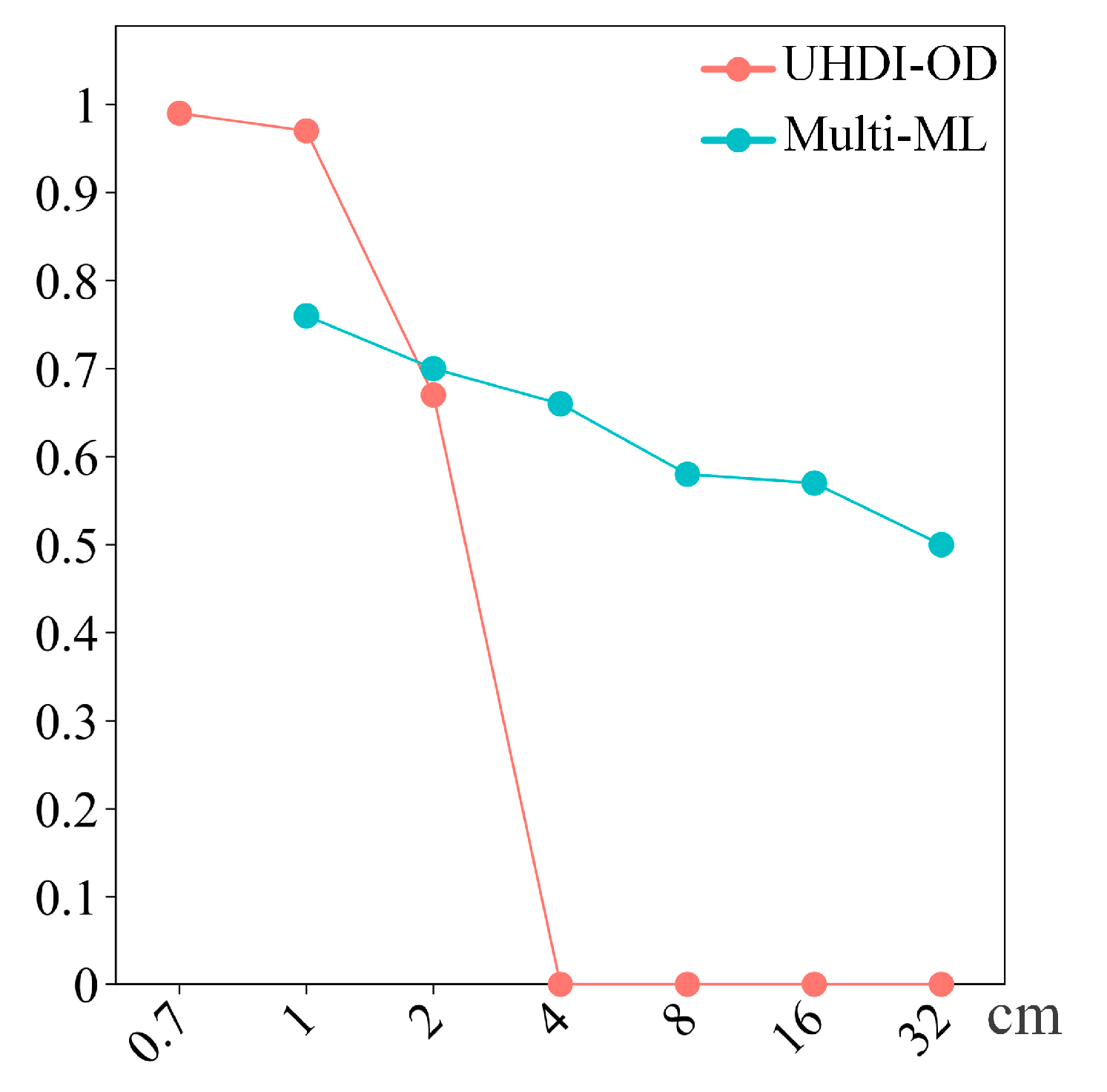
4.3.1. Comparison of the Maize Planting Density Estimation Results at Different Resolutions

The pixel size of the original digital images is 0.7 cm and the pixel size of the original multispectral images is 1 cm. Through resampling, this study adjusted the pixel sizes of both the digital and multispectral images to 1 cm, 2 cm, 4 cm, 8 cm, 16 cm, and 32 cm, to investigate the impact of resolution on the estimation accuracies (measured using R²) of the two methods (UHDI-OD and Multi-ML). The results are shown in Figure 9. Both methods were trained on images at their respective original resolutions and the best models were directly used to estimate the planting density of 790 plots. When the pixel size was less than 2 cm, the accuracies of UHDI-OD are higher than that of Multi-ML. However, when the pixel sizes exceeded 2 cm, the accuracies of UHDI-OD rapidly decreased to 0, while the accuracies of Multi-ML remained above 0.5. This indicates that the image resolution significantly affects UHDI-OD, especially at lower resolutions, where its performance is noticeably constrained. In contrast, Multi-ML maintains relatively stable estimation accuracies across different resolutions, demonstrating good adaptability to resolution changes.

4.3.2. Analysis of Model Advantages in Different Application Scenarios

During the data training phase, UHDI-OD, which employs a deep learning architecture, requires large models and high-performance computing devices, resulting in a slower training process (

Table 5. Method comparison results.

	UHDI-OD	Multi-ML
Data training	Deep learning model, slow training speed (50 min), high-performance computing equipment	Relatively simple model, fast training speed (0.2 min)
Estimate accuracy	YOLOv8, higher accuracy (R2 = 0.99)	RF regression model, lower accuracy (R2 = 0.76)
Universality	Easily affected by resolution interference (R2 drops to 0 when the pixel size is reduced to 4 cm)	Adapt to different resolutions (R2 can still remain above 0.50 when the pixel size is reduced to 32 cm)
Scope of application	Small area density monitoring	Large area density monitoring

, 50 min). In contrast, Multi-ML, which uses relatively simple regression models, yields faster training speeds (Table 5, 0.2 min) with lower computational device requirements. In terms of the estimation accuracy, UHDI-OD (Table 5, R² = 0.99) outperforms Multi-ML (Table 5, R² = 0.76). Furthermore, regarding the universality, UHDI-OD shows poorer adaptability at different resolutions (Table 5, decreasing to 0 when the pixel size is increased to 4 cm). Conversely, the spectral information in Multi-ML demonstrates excellent performance at various resolutions (Table 5, maintaining R² values above 0.50, even when the pixel size is increased to 32 cm), indicating stronger universality. In mapping, UHDI-OD requires determining the maize quantities before calculating the densities, while Multi-ML directly estimates the planting densities, simplifying the mapping process. Therefore, this study speculates that UHDI-OD is suitable for density monitoring small areas, whereas Multi-ML is more suitable for density monitoring large areas (Table 5).

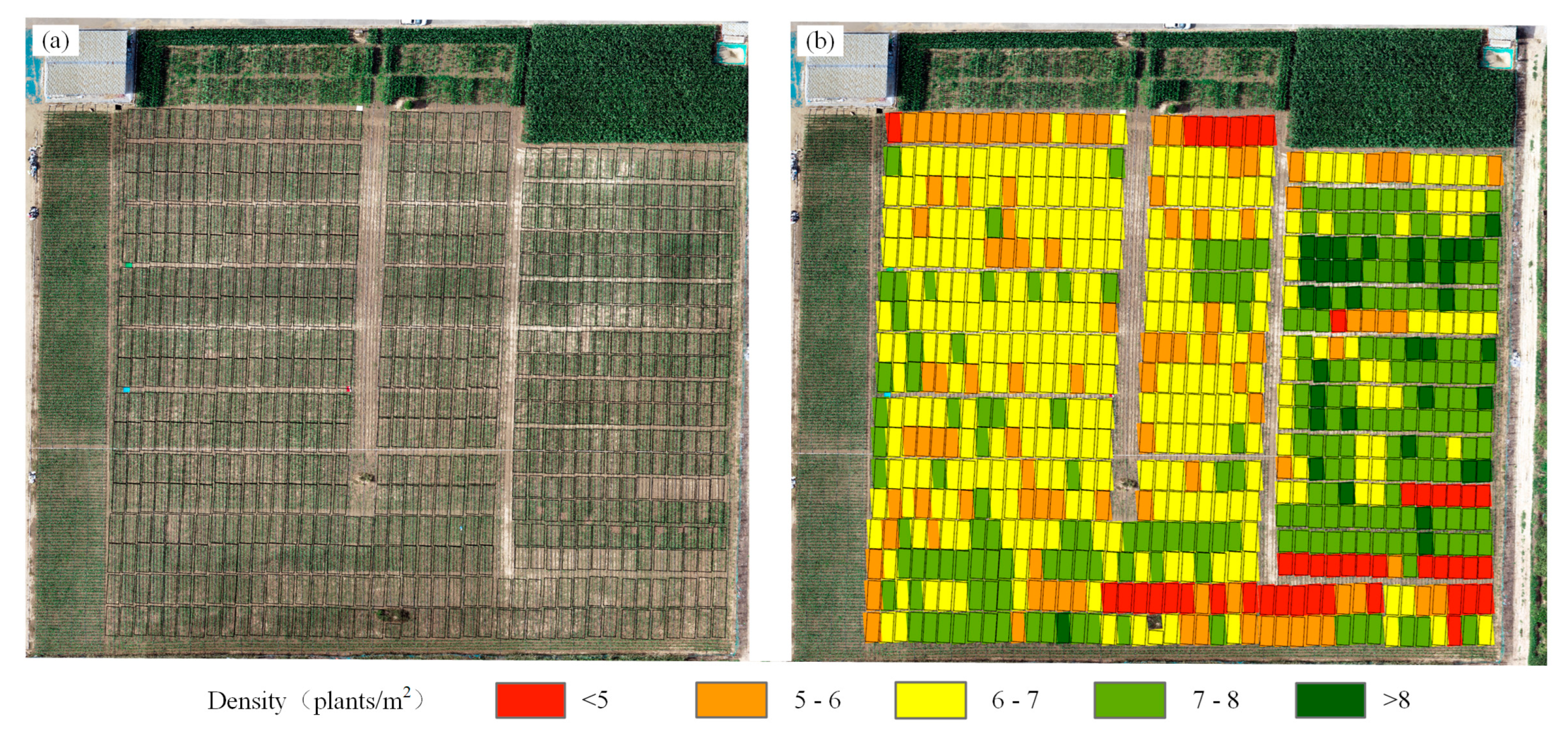
4.4. Multi-ML for Mapping Maize Planting Densities

UHDI-OD typically requires a prior determination of the maize quantities, followed by calculations of the densities. In this process, obtaining actual area information is crucial for ensuring accurate estimations of the planting densities. In contrast, Multi-ML directly acquires the planting densities through the output of the regression model without being constrained by the size of the study area. This approach enhances the convenience and accuracy of mapping since no additional area information is needed. The density information is estimated directly from the results of the regression model, simplifying the data processing workflow and thereby improving the generalizability and applicability of the method. Therefore, this study employs Multi-ML for mapping, as illustrated in Figure 10.

5. Discussion

5.1. Advantages of the Proposed Methods

Previous studies in crop quantity estimation with ultrahigh-definition digital images primarily used deep learning techniques. For instance, Vong et al. and Gao et al. [35] employed the U-Net and Mask R-CNN models, respectively, for image segmentation. In another approach involving the use of object detection techniques in deep learning, Liu et al. [34] selected YOLOv3, while Xu et al. [36] and Cardellicchio et al. [67] opted for YOLOv5 for accurate crop quantity estimations. In this study, UHDI-OD employed YOLOv8 for maize object detection and, subsequently, when combined with the measured planting areas, the maize planting densities were obtained (Figure 6). However, acquiring ultrahigh-definition digital images typically involves low-altitude drone flights, incurring substantial time and manpower costs. In order to solve this problem, this study proposes Multi-ML as a more cost-effective solution.

Multi-ML uses multispectral data for maize planting density estimations (Table 4). Compared to ultrahigh-definition digital images, multispectral data have more spectral bands. However, it is essential to note that the resolution of multispectral imaging systems is relatively limited, which makes it challenging to accurately distinguish individual maize plants. As a result, some studies suggest combining spectral VIs information for crop quantity and density extractions [51,52,53]. While this approach has been implemented for crops such as wheat [68] and soybeans [69], its application in maize planting density estimations is scarce. Therefore, this study attempted to estimate the maize planting densities using multispectral VIs. Additionally, this study processed the five original bands of multispectral data through the GLCM, which revealed significant improvements in the correlations among the original bands and the planting densities after GLCM processing (Figure 7). Consequently, the study combined the textural features obtained using the GLCM with the VIs for maize planting density estimations, and revealed that the combination of VIs and textural features yielded a greater estimation accuracy (Figure 8).

5.2. Applicable Scenarios of the Proposed Methods

While Multi-ML attempted to increase the accuracy of maize planting density estimations by combining the VIs and textural features (R² = 0.76, RMSE = 0.67 plants/m²), UHDI-OD still retained higher accuracy maize planting density estimations (R² = 0.99, RMSE = 0.09 plants/m²). However, the precision of UHDI-OD requires complex data processing and model training. For instance, UHDI-OD not only requires measurements of ground data, but also requires a manual annotation of the position of each maize plant. Additionally, training YOLO models imposes certain demands on computational resources. In previous studies applying deep learning models for maize quantity estimations, the UAV flight heights were typically chosen to be in the range of 5–20 m [34,36,70], indicating the strict requirements of the UHDI-OD method for ultrahigh-definition digital images. Acquiring such ultrahigh-definition digital images often involves the use of UAV-carried RGB digital cameras for low-altitude image collection, which might pose challenges for monitoring large-scale field planting densities within a reasonable period.

This study also revealed that during the use of UHDI-OD, the maize planting density estimation results rapidly deteriorated as the resolution decreased. In contrast, Multi-ML has lower resolution requirements and a reduction in resolution still maintains the estimation accuracy (Figure 9). While UHDI-OD achieved higher accuracy in the maize planting density estimations, Multi-ML demonstrated more cost-effective advantages in large-scale field monitoring. These conclusions provide strong guidance for selecting appropriate data sources and methods, as well as for decision-making in field monitoring.

5.3. Disadvantages of the Proposed Methods

Although this study developed two methods that provided a comprehensive solution for monitoring maize planting densities, there were still some shortcomings and potential areas for improvement.

(1)

This study tested two methods using simulated low-resolution images, which may not fully reflect the impacts of actual scene changes in the image resolution on model performance. Future research could consider collecting real low-resolution images to more accurately assess the model performance in practical applications.

(2)

This study did not thoroughly consider the monitoring results for maize at different time points or account for situations where the maize plants were smaller or partially occluded. In future studies, a detailed analysis of maize monitoring at different growth stages and considering the detection challenges in complex scenarios could enhance the applicability of the method.

(3)

This study conducted tests only in specific regions and for a specific crop (maize). Future research should broaden the scope of the field by considering different geographical regions and crop types to comprehensively evaluate the strengths, weaknesses, and feasibility of both methods.

6. Conclusions

This study developed two maize planting density monitoring methods using UAV remote sensing, namely UHDI-OD and Multi-ML. UHDI-OD achieved highly accurate results (R² = 0.99, RMSE = 0.09 plants/m²) and showed promising precision in recognizing maize objects. Multi-ML, combining VIs and GLCM texture features, yielded higher-precision results (R² = 0.76, RMSE = 0.67 plants/m²), with the RF model performing optimally. While UHDI-OD is sensitive to image resolution and not suitable for UAV images with pixel sizes exceeding 2 cm, Multi-ML is less sensitive to resolution, offering greater convenience and cost-effectiveness for large-scale field monitoring. Therefore, although UHDI-OD achieves higher accuracy, Multi-ML has more cost-effective advantages in large-scale field monitoring. While this study has introduced two methods for monitoring maize planting densities, there remain areas for improvement. Future research should focus on refining model performance with real low-resolution images, incorporating temporal dynamics for comprehensive monitoring, and expanding the scope to different regions and crop types for broader applicability.

References

- Ranum, P.; Peña-Rosas, J.P.; Garcia-Casal, M.N. Global Maize Production, Utilization, and Consumption. Ann. N. Y. Acad. Sci. 2014, 1312, 105–112. [Google Scholar] [CrossRef]
- Shu, G.; Cao, G.; Li, N.; Wang, A.; Wei, F.; Li, T.; Yi, L.; Xu, Y.; Wang, Y. Genetic Variation and Population Structure in China Summer Maize Germplasm. Sci. Rep. 2021, 11, 8012. [Google Scholar] [CrossRef]
- Ghasemi, A.; Azarfar, A.; Omidi-Mirzaei, H.; Fadayifar, A.; Hashemzadeh, F.; Ghaffari, M.H. Effects of Corn Processing Index and Forage Source on Performance, Blood Parameters, and Ruminal Fermentation of Dairy Calves. Sci. Rep. 2023, 13, 17914. [Google Scholar] [CrossRef]
- Shirzadifar, A.; Maharlooei, M.; Bajwa, S.G.; Oduor, P.G.; Nowatzki, J.F. Mapping Crop Stand Count and Planting Uniformity Using High Resolution Imagery in a Maize Crop. Biosyst. Eng. 2020, 200, 377–390. [Google Scholar] [CrossRef]
- Van Roekel, R.J.; Coulter, J.A. Agronomic Responses of Corn to Planting Date and Plant Density. Agron. J. 2011, 103, 1414–1422. [Google Scholar] [CrossRef]
- Gnädinger, F.; Schmidhalter, U. Digital Counts of Maize Plants by Unmanned Aerial Vehicles (UAVs). Remote Sens. 2017, 9, 544. [Google Scholar] [CrossRef]
- Yue, J.; Zhou, C.; Guo, W.; Feng, H.; Xu, K. Estimation of Winter-Wheat above-Ground Biomass Using the Wavelet Analysis of Unmanned Aerial Vehicle-Based Digital Images and Hyperspectral Crop Canopy Images. Int. J. Remote Sens. 2021, 42, 1602–1622. [Google Scholar] [CrossRef]
- Liu, Y.; Feng, H.; Yue, J.; Jin, X.; Fan, Y.; Chen, R.; Bian, M.; Ma, Y.; Song, X.; Yang, G. Improved Potato AGB Estimates Based on UAV RGB and Hyperspectral Images. Comput. Electron. Agric. 2023, 214, 108260. [Google Scholar] [CrossRef]
- Maes, W.H.; Steppe, K. Perspectives for Remote Sensing with Unmanned Aerial Vehicles in Precision Agriculture. Trends Plant Sci. 2019, 24, 152–164. [Google Scholar] [CrossRef]
- Colomina, I.; Molina, P. Unmanned Aerial Systems for Photogrammetry and Remote Sensing: A Review. ISPRS J. Photogramm. Remote Sens. 2014, 92, 79–97. [Google Scholar] [CrossRef]
- Sassu, A.; Motta, J.; Deidda, A.; Ghiani, L.; Carlevaro, A.; Garibotto, G.; Gambella, F. Artichoke Deep Learning Detection Network for Site-Specific Agrochemicals UAS Spraying. Comput. Electron. Agric. 2023, 213, 108185. [Google Scholar] [CrossRef]
- Shakhatreh, H.; Sawalmeh, A.H.; Al-Fuqaha, A.; Dou, Z.; Almaita, E.; Khalil, I.; Othman, N.S.; Khreishah, A.; Guizani, M. Unmanned Aerial Vehicles (UAVs): A Survey on Civil Applications and Key Research Challenges. IEEE Access 2019, 7, 48572–48634. [Google Scholar] [CrossRef]
- Liu, Y.; Feng, H.; Yue, J.; Fan, Y.; Bian, M.; Ma, Y.; Jin, X.; Song, X.; Yang, G. Estimating Potato Above-Ground Biomass by Using Integrated Unmanned Aerial System-Based Optical, Structural, and Textural Canopy Measurements. Comput. Electron. Agric. 2023, 213, 108229. [Google Scholar] [CrossRef]
- Yue, J.; Feng, H.; Li, Z.; Zhou, C.; Xu, K. Mapping Winter-Wheat Biomass and Grain Yield Based on a Crop Model and UAV Remote Sensing. Int. J. Remote Sens. 2021, 42, 1577–1601. [Google Scholar] [CrossRef]
- Yue, J.; Yang, G.; Li, C.; Li, Z.; Wang, Y.; Feng, H.; Xu, B. Estimation of Winter Wheat Above-Ground Biomass Using Unmanned Aerial Vehicle-Based Snapshot Hyperspectral Sensor and Crop Height Improved Models. Remote Sens. 2017, 9, 708. [Google Scholar] [CrossRef]
- Zhu, L.; Li, X.; Sun, H.; Han, Y. Research on CBF-YOLO Detection Model for Common Soybean Pests in Complex Environment. Comput. Electron. Agric. 2024, 216, 108515. [Google Scholar] [CrossRef]
- Zhang, Z.; Khanal, S.; Raudenbush, A.; Tilmon, K.; Stewart, C. Assessing the Efficacy of Machine Learning Techniques to Characterize Soybean Defoliation from Unmanned Aerial Vehicles. Comput. Electron. Agric. 2022, 193, 106682. [Google Scholar] [CrossRef]
- Guo, Y.; Fu, Y.H.; Chen, S.; Robin Bryant, C.; Li, X.; Senthilnath, J.; Sun, H.; Wang, S.; Wu, Z.; de Beurs, K. Integrating Spectral and Textural Information for Identifying the Tasseling Date of Summer Maize Using UAV Based RGB Images. Int. J. Appl. Earth Obs. Geoinf. 2021, 102, 102435. [Google Scholar] [CrossRef]
- Jin, X.; Liu, S.; Baret, F.; Hemerlé, M.; Comar, A. Estimates of Plant Density of Wheat Crops at Emergence from Very Low Altitude UAV Imagery. Remote Sens. Environ. 2017, 198, 105–114. [Google Scholar] [CrossRef]
- Yu, N.; Li, L.; Schmitz, N.; Tian, L.F.; Greenberg, J.A.; Diers, B.W. Development of Methods to Improve Soybean Yield Estimation and Predict Plant Maturity with an Unmanned Aerial Vehicle Based Platform. Remote Sens. Environ. 2016, 187, 91–101. [Google Scholar] [CrossRef]
- Etienne, A.; Ahmad, A.; Aggarwal, V.; Saraswat, D. Deep Learning-Based Object Detection System for Identifying Weeds Using UAS Imagery. Remote Sens. 2021, 13, 5182. [Google Scholar] [CrossRef]
- Xiao, J.; Suab, S.A.; Chen, X.; Singh, C.K.; Singh, D.; Aggarwal, A.K.; Korom, A.; Widyatmanti, W.; Mollah, T.H.; Minh, H.V.T.; et al. Enhancing Assessment of Corn Growth Performance Using Unmanned Aerial Vehicles (UAVs) and Deep Learning. Measurement 2023, 214, 112764. [Google Scholar] [CrossRef]
- Liu, S.; Baret, F.; Andrieu, B.; Burger, P.; Hemmerlé, M. Estimation of Wheat Plant Density at Early Stages Using High Resolution Imagery. Front. Plant Sci. 2017, 8, 739. [Google Scholar] [CrossRef]
- Yang, Q.; Shi, L.; Han, J.; Yu, J.; Huang, K. A near Real-Time Deep Learning Approach for Detecting Rice Phenology Based on UAV Images. Agric. For. Meteorol. 2020, 287, 107938. [Google Scholar] [CrossRef]
- Lin, Y.; Chen, T.; Liu, S.; Cai, Y.; Shi, H.; Zheng, D.; Lan, Y.; Yue, X.; Zhang, L. Quick and Accurate Monitoring Peanut Seedlings Emergence Rate through UAV Video and Deep Learning. Comput. Electron. Agric. 2022, 197, 106938. [Google Scholar] [CrossRef]
- Li, B.; Xu, X.; Han, J.; Zhang, L.; Bian, C.; Jin, L.; Liu, J. The Estimation of Crop Emergence in Potatoes by UAV RGB Imagery. Plant Methods 2019, 15, 15. [Google Scholar] [CrossRef]
- Krizhevsky, A.; Sutskever, I.; Hinton, G.E. ImageNet Classification with Deep Convolutional Neural Networks. Commun. ACM 2017, 60, 84–90. [Google Scholar] [CrossRef]
- Simonyan, K.; Zisserman, A. Very Deep Convolutional Networks for Large-Scale Image Recognition. arXiv 2014, arXiv:1409.1556. [Google Scholar]
- He, K.; Zhang, X.; Ren, S.; Sun, J. Deep Residual Learning for Image Recognition. In Proceedings of the 2016 IEEE Conference on Computer Vision and Pattern Recognition (CVPR), Las Vegas, NV, USA, 27–30 June 2016; pp. 770–778. [Google Scholar]
- Fan, Z.; Lu, J.; Gong, M.; Xie, H.; Goodman, E.D. Automatic Tobacco Plant Detection in UAV Images via Deep Neural Networks. IEEE J. Sel. Top. Appl. Earth Obs. Remote Sens. 2018, 11, 876–887. [Google Scholar] [CrossRef]
- Guo, W.; Zheng, B.; Potgieter, A.B.; Diot, J.; Watanabe, K.; Noshita, K.; Jordan, D.R.; Wang, X.; Watson, J.; Ninomiya, S.; et al. Aerial Imagery Analysis—Quantifying Appearance and Number of Sorghum Heads for Applications in Breeding and Agronomy. Front. Plant Sci. 2018, 9, 1544. [Google Scholar] [CrossRef]
- Fuentes, A.; Yoon, S.; Kim, S.C.; Park, D.S. A Robust Deep-Learning-Based Detector for Real-Time Tomato Plant Diseases and Pests Recognition. Sensors 2017, 17, 2022. [Google Scholar] [CrossRef] [PubMed]
- Sa, I.; Ge, Z.; Dayoub, F.; Upcroft, B.; Perez, T.; McCool, C. DeepFruits: A Fruit Detection System Using Deep Neural Networks. Sensors 2016, 16, 1222. [Google Scholar] [CrossRef] [PubMed]
- Liu, M.; Su, W.-H.; Wang, X.-Q. Quantitative Evaluation of Maize Emergence Using UAV Imagery and Deep Learning. Remote Sens. 2023, 15, 1979. [Google Scholar] [CrossRef]
- Gao, X.; Zan, X.; Yang, S.; Zhang, R.; Chen, S.; Zhang, X.; Liu, Z.; Ma, Y.; Zhao, Y.; Li, S. Maize Seedling Information Extraction from UAV Images Based on Semi-Automatic Sample Generation and Mask R-CNN Model. Eur. J. Agron. 2023, 147, 126845. [Google Scholar] [CrossRef]
- Xu, X.; Wang, L.; Liang, X.; Zhou, L.; Chen, Y.; Feng, P.; Yu, H.; Ma, Y. Maize Seedling Leave Counting Based on Semi-Supervised Learning and UAV RGB Images. Sustainability 2023, 15, 9583. [Google Scholar] [CrossRef]
- Osco, L.P.; dos Santos de Arruda, M.; Gonçalves, D.N.; Dias, A.; Batistoti, J.; de Souza, M.; Gomes, F.D.G.; Ramos, A.P.M.; de Castro Jorge, L.A.; Liesenberg, V.; et al. A CNN Approach to Simultaneously Count Plants and Detect Plantation-Rows from UAV Imagery. ISPRS J. Photogramm. Remote Sens. 2021, 174, 1–17. [Google Scholar] [CrossRef]
- Vong, C.N.; Conway, L.S.; Zhou, J.; Kitchen, N.R.; Sudduth, K.A. Early Corn Stand Count of Different Cropping Systems Using UAV-Imagery and Deep Learning. Comput. Electron. Agric. 2021, 186, 106214. [Google Scholar] [CrossRef]
- Springenberg, J.T.; Dosovitskiy, A.; Brox, T.; Riedmiller, M. Striving for Simplicity: The All Convolutional Net 2015. arXiv 2014, arXiv:1412.6806. [Google Scholar]
- Espejo-Garcia, B.; Mylonas, N.; Athanasakos, L.; Fountas, S. Improving Weeds Identification with a Repository of Agricultural Pre-Trained Deep Neural Networks. Comput. Electron. Agric. 2020, 175, 105593. [Google Scholar] [CrossRef]
- Feng, A.; Zhou, J.; Vories, E.; Sudduth, K.A. Evaluation of Cotton Emergence Using UAV-Based Imagery and Deep Learning. Comput. Electron. Agric. 2020, 177, 105711. [Google Scholar] [CrossRef]
- Zhou, C.; Hu, J.; Xu, Z.; Yue, J.; Ye, H.; Yang, G. A Monitoring System for the Segmentation and Grading of Broccoli Head Based on Deep Learning and Neural Networks. Front. Plant Sci. 2020, 11, 402. [Google Scholar] [CrossRef] [PubMed]
- Hu, J.; Yue, J.; Xu, X.; Han, S.; Sun, T.; Liu, Y.; Feng, H.; Qiao, H. UAV-Based Remote Sensing for Soybean FVC, LCC, and Maturity Monitoring. Agriculture 2023, 13, 692. [Google Scholar] [CrossRef]
- Yue, J.; Guo, W.; Yang, G.; Zhou, C.; Feng, H.; Qiao, H. Method for Accurate Multi-Growth-Stage Estimation of Fractional Vegetation Cover Using Unmanned Aerial Vehicle Remote Sensing. Plant Methods 2021, 17, 51. [Google Scholar] [CrossRef] [PubMed]
- Yue, J.; Yang, H.; Yang, G.; Fu, Y.; Wang, H.; Zhou, C. Estimating Vertically Growing Crop Above-Ground Biomass Based on UAV Remote Sensing. Comput. Electron. Agric. 2023, 205, 107627. [Google Scholar] [CrossRef]
- Bendig, J.; Yu, K.; Aasen, H.; Bolten, A.; Bennertz, S.; Broscheit, J.; Gnyp, M.L.; Bareth, G. Combining UAV-Based Plant Height from Crop Surface Models, Visible, and near Infrared Vegetation Indices for Biomass Monitoring in Barley. Int. J. Appl. Earth Obs. Geoinf. 2015, 39, 79–87. [Google Scholar] [CrossRef]
- Liu, Y.; Feng, H.; Yue, J.; Jin, X.; Li, Z.; Yang, G. Estimation of Potato Above-Ground Biomass Based on Unmanned Aerial Vehicle Red-Green-Blue Images with Different Texture Features and Crop Height. Front. Plant Sci. 2022, 13, 938216. [Google Scholar] [CrossRef] [PubMed]
- Qiao, L.; Zhao, R.; Tang, W.; An, L.; Sun, H.; Li, M.; Wang, N.; Liu, Y.; Liu, G. Estimating Maize LAI by Exploring Deep Features of Vegetation Index Map from UAV Multispectral Images. Field Crops Res. 2022, 289, 108739. [Google Scholar] [CrossRef]
- Fan, Y.; Feng, H.; Jin, X.; Yue, J.; Liu, Y.; Li, Z.; Feng, Z.; Song, X.; Yang, G. Estimation of the Nitrogen Content of Potato Plants Based on Morphological Parameters and Visible Light Vegetation Indices. Front. Plant Sci. 2022, 13, 1012070. [Google Scholar] [CrossRef] [PubMed]
- Yue, J.; Tian, J.; Philpot, W.; Tian, Q.; Feng, H.; Fu, Y. VNAI-NDVI-Space and Polar Coordinate Method for Assessing Crop Leaf Chlorophyll Content and Fractional Cover. Comput. Electron. Agric. 2023, 207, 107758. [Google Scholar] [CrossRef]
- Sankaran, S.; Khot, L.R.; Carter, A.H. Field-Based Crop Phenotyping: Multispectral Aerial Imaging for Evaluation of Winter Wheat Emergence and Spring Stand. Comput. Electron. Agric. 2015, 118, 372–379. [Google Scholar] [CrossRef]
- Banerjee, B.P.; Sharma, V.; Spangenberg, G.; Kant, S. Machine Learning Regression Analysis for Estimation of Crop Emergence Using Multispectral UAV Imagery. Remote Sens. 2021, 13, 2918. [Google Scholar] [CrossRef]
- Wilke, N.; Siegmann, B.; Postma, J.A.; Muller, O.; Krieger, V.; Pude, R.; Rascher, U. Assessment of Plant Density for Barley and Wheat Using UAV Multispectral Imagery for High-Throughput Field Phenotyping. Comput. Electron. Agric. 2021, 189, 106380. [Google Scholar] [CrossRef]
- Lee, H.; Wang, J.; Leblon, B. Using Linear Regression, Random Forests, and Support Vector Machine with Unmanned Aerial Vehicle Multispectral Images to Predict Canopy Nitrogen Weight in Corn. Remote Sens. 2020, 12, 2071. [Google Scholar] [CrossRef]
- Redmon, J.; Divvala, S.; Girshick, R.; Farhadi, A. You Only Look Once: Unified, Real-Time Object Detection 2016. In Proceedings of the IEEE Conference on Computer Vision and Pattern Recognition (CVPR), Las Vegas, NV, USA, 27–30 June 2016. [Google Scholar]
- Zhu, X.; Lyu, S.; Wang, X.; Zhao, Q. TPH-YOLOv5: Improved YOLOv5 Based on Transformer Prediction Head for Object Detection on Drone-Captured Scenarios 2021. In Proceedings of the IEEE/CVF International Conference on Computer Vision (ICCV) Workshops, Montreal, QC, Canada, 10–17 October 2021. [Google Scholar]
- Redmon, J.; Farhadi, A. YOLOv3: An Incremental Improvement 2018. arXiv 2018, arXiv:1804.02767. [Google Scholar]
- Selvaraju, R.R.; Cogswell, M.; Das, A.; Vedantam, R.; Parikh, D.; Batra, D. Grad-CAM: Visual Explanations from Deep Networks via Gradient-Based Localization. Int. J. Comput. Vis. 2020, 128, 336–359. [Google Scholar] [CrossRef]
- Chattopadhyay, A.; Sarkar, A.; Howlader, P.; Balasubramanian, V.N. Grad-CAM++: Improved Visual Explanations for Deep Convolutional Networks. In Proceedings of the 2018 IEEE Winter Conference on Applications of Computer Vision (WACV), Lake Tahoe, NV, USA, 12–15 March 2018; pp. 839–847. [Google Scholar]
- Fu, R.; Hu, Q.; Dong, X.; Guo, Y.; Gao, Y.; Li, B. Axiom-Based Grad-CAM: Towards Accurate Visualization and Explanation of CNNs 2020. arXiv 2020, arXiv:2008.02312. [Google Scholar]
- Freden, S.C.; Mercanti, E.P.; Becker, M.A. (Eds.) Third Earth Resources Technology Satellite-1 Symposium: Section A-B; Technical Presentations; Scientific and Technical Information Office, National Aeronautics and Space Administration: Washington, DC, USA, 1973. [Google Scholar]
- Rondeaux, G.; Steven, M.; Baret, F. Optimization of Soil-Adjusted Vegetation Indices. Remote Sens. Environ. 1996, 55, 95–107. [Google Scholar] [CrossRef]
- Datt, B. A New Reflectance Index for Remote Sensing of Chlorophyll Content in Higher Plants: Tests Using Eucalyptus Leaves. J. Plant Physiol. 1999, 154, 30–36. [Google Scholar] [CrossRef]
- Gitelson, A.A.; Kaufman, Y.J.; Merzlyak, M.N. Use of a Green Channel in Remote Sensing of Global Vegetation from EOS-MODIS. Remote Sens. Environ. 1996, 58, 289–298. [Google Scholar] [CrossRef]
- Gitelson, A.; Merzlyak, M.N. Spectral Reflectance Changes Associated with Autumn Senescence of Aesculus hippocastanum L. and Acer platanoides L. Leaves. Spectral Features and Relation to Chlorophyll Estimation. J. Plant Physiol. 1994, 143, 286–292. [Google Scholar] [CrossRef]
- Haralick, R.M.; Shanmugam, K.; Dinstein, I. Textural Features for Image Classification. IEEE Trans. Syst. Man. Cybern. 1973, SMC-3, 610–621. [Google Scholar] [CrossRef]
- Cardellicchio, A.; Solimani, F.; Dimauro, G.; Petrozza, A.; Summerer, S.; Cellini, F.; Renò, V. Detection of Tomato Plant Phenotyping Traits Using YOLOv5-Based Single Stage Detectors. Comput. Electron. Agric. 2023, 207, 107757. [Google Scholar] [CrossRef]
- Yang, T.; Jay, S.; Gao, Y.; Liu, S.; Baret, F. The Balance between Spectral and Spatial Information to Estimate Straw Cereal Plant Density at Early Growth Stages from Optical Sensors. Comput. Electron. Agric. 2023, 215, 108458. [Google Scholar] [CrossRef]
- Habibi, L.N.; Watanabe, T.; Matsui, T.; Tanaka, T.S.T. Machine Learning Techniques to Predict Soybean Plant Density Using UAV and Satellite-Based Remote Sensing. Remote Sens. 2021, 13, 2548. [Google Scholar] [CrossRef]
- Vong, C.N.; Conway, L.S.; Feng, A.; Zhou, J.; Kitchen, N.R.; Sudduth, K.A. Corn Emergence Uniformity Estimation and Mapping Using UAV Imagery and Deep Learning. Comput. Electron. Agric. 2022, 198, 107008. [Google Scholar] [CrossRef]