
A Hierarchical Neural Network for Point Cloud Segmentation and Geometric Primitive Fitting

Abstract
:1. Introduction
- This study introduces an innovative feature extraction network that is specifically designed to address the issue of imprecision that arises during the process of geometric primitive recognition.
- We propose a parameter prediction module, the design of which is intended to predict the parameters of geometric primitives more accurately. This is crucial for enhancing the precision of shape representation and for the understanding of complex 3D structures, marking an important step toward fine-grained 3D modeling.
- Extensive experimental validation demonstrates that our method shows significant advantages in terms of accuracy. These experimental results fully substantiate the effectiveness and practicality of our model in the processing of 3D geometric data, providing reliable technical support for further research and practical applications in the field of computer vision.
2. Related Work
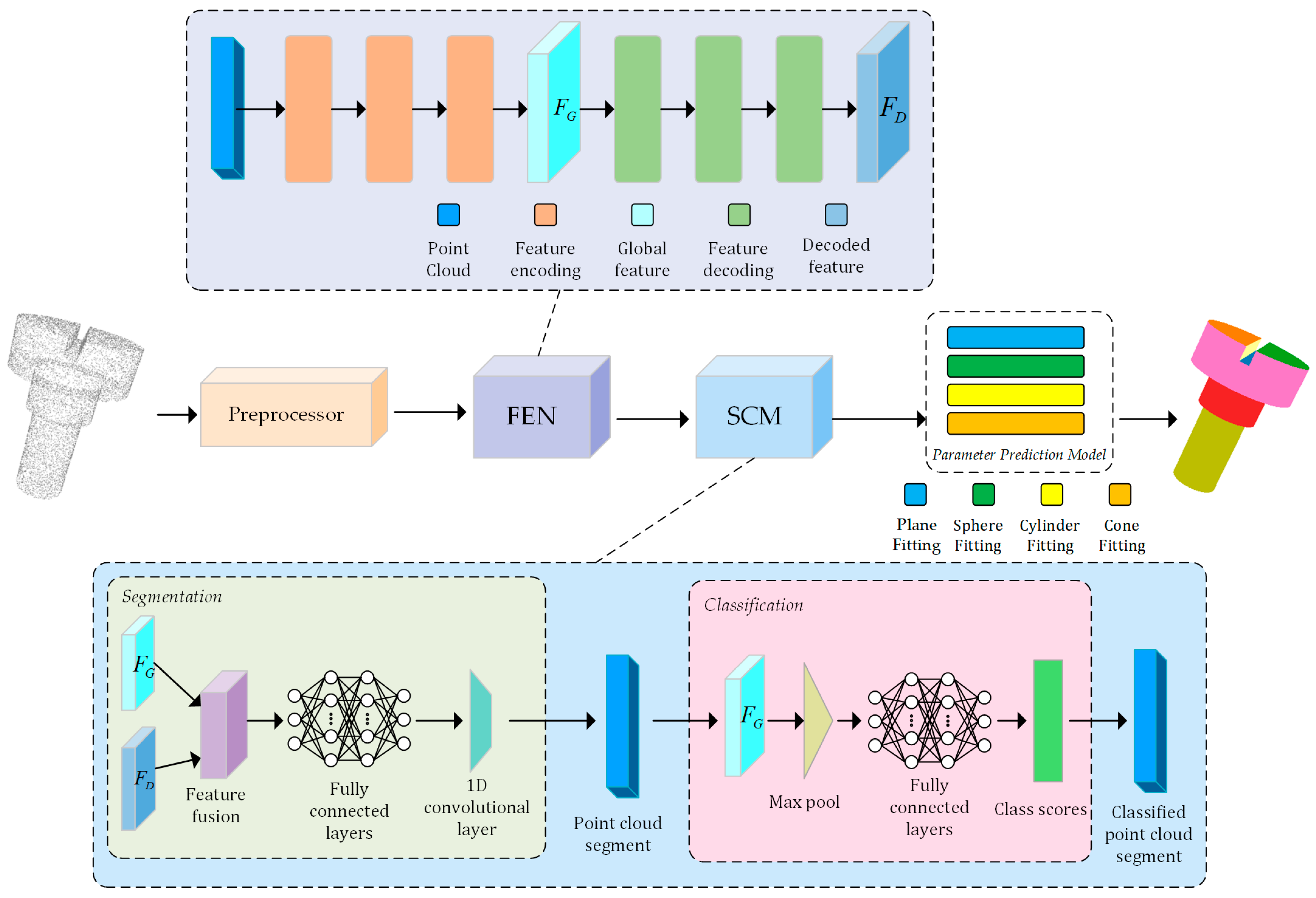
3. Method
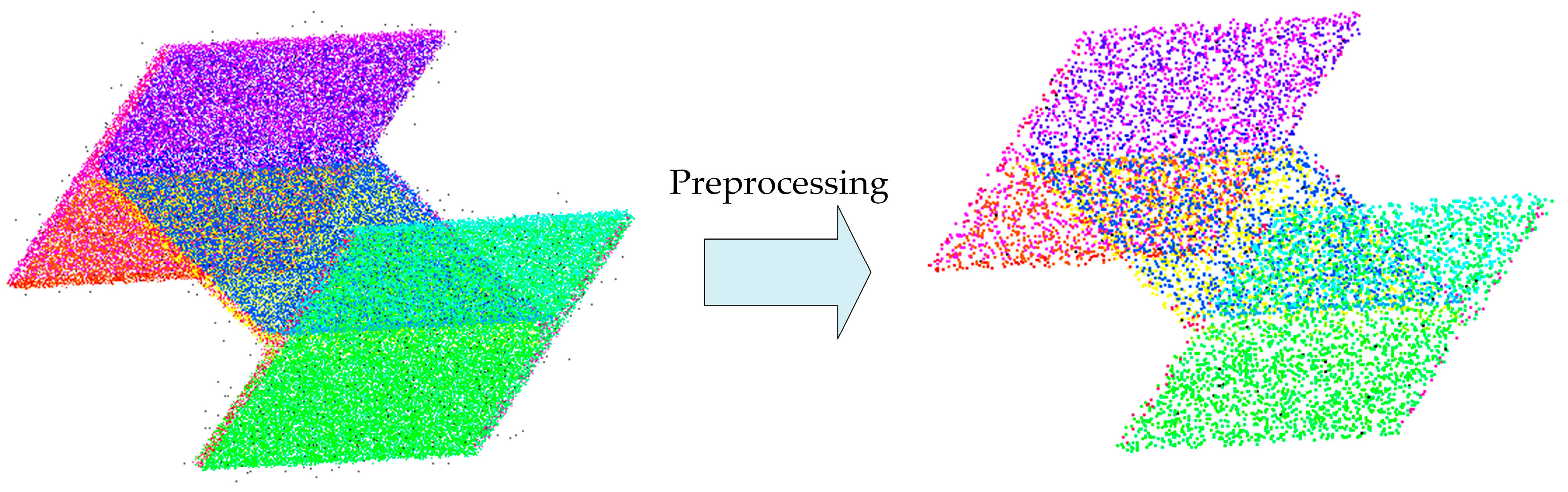
3.1. Preprocessing Module
3.2. Feature Extraction Network (FEN)
3.2.1. Input and Output
3.2.2. Sampling Layer
3.2.3. Grouping Layer
3.2.4. PointConv Layer
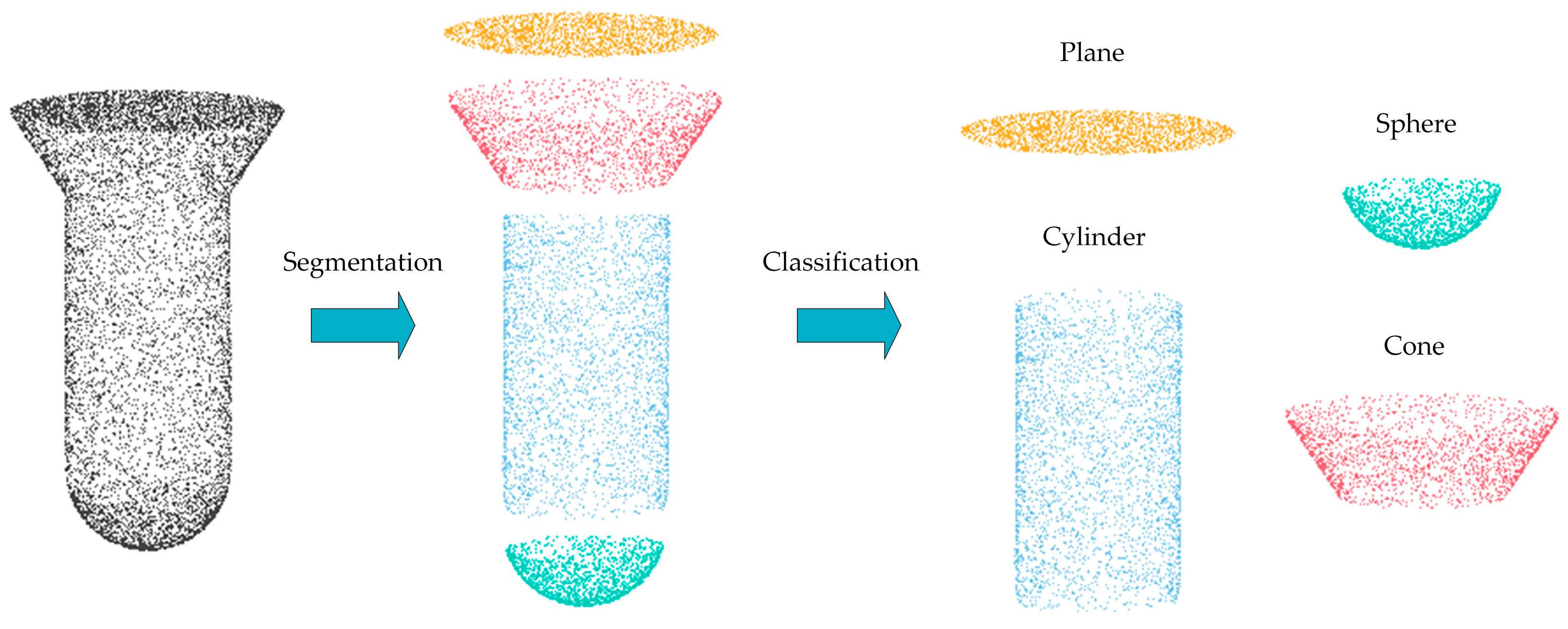
3.3. Segmentation and Classification Module (SCM)
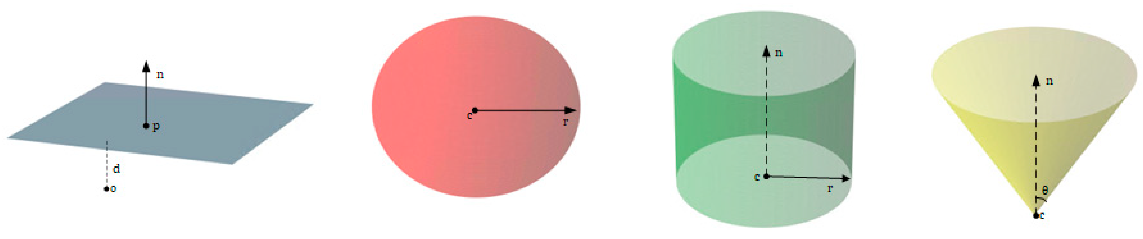
3.4. Parameter Prediction Model
3.4.1. Plane
3.4.2. Sphere
3.4.3. Cylinder
3.4.4. Cone
3.5. Evaluation Metrics
- Segmentation mean intersection over union (IoU)
- 2.
- Mean primitive type accuracy
- 3.
- Mean point normal difference
- 4.
- Mean primitive axis difference
- 5.
- Mean residual
- 6
- P coverage
4. Experiments
5. Conclusions
Author Contributions
Funding
Institutional Review Board Statement
Data Availability Statement
Conflicts of Interest
References
- Morteza, D.; Ahmed, H.; Egils, A.; Fatemeh, N.; Fatih, A.; Hasan, S.A.; Jelena, G.; Rain, E.H.; Cagri, O.; Gholamreza, A. 3D scanning: A comprehensive survey. arXiv 2018, arXiv:1801.08863. [Google Scholar] [CrossRef]
- Fayolle, P.-A.; Friedrich, M. A Survey of Methods for Converting Unstructured Data to CSG Models. Comput. Aided Des. 2024, 168, 103655. [Google Scholar] [CrossRef]
- Sergiyenko, O.; Alaniz-Plata, R.; Flores-Fuentes, W.; Rodríguez-Quiñonez, J.C.; Miranda-Vega, J.E.; Sepulveda-Valdez, C.; Núñez-López, J.A.; Kolendovska, M.; Kartashov, V.; Tyrsa, V. Multi-view 3D data fusion and patching to reduce Shannon entropy in Robotic Vision. Opt. Lasers Eng. 2024, 177, 108132. [Google Scholar] [CrossRef]
- Chum, O.; Matas, J. Optimal randomized RANSAC. IEEE Trans. Pattern Anal. Mach. Intell. 2008, 30, 1472–1482. [Google Scholar] [CrossRef] [PubMed]
- Li, L.; Sung, M.; Dubrovina, A.; Yi, L.; Guibas, L.J. Supervised fitting of geometric primitives to 3d point clouds. In Proceedings of the IEEE/CVF Conference on Computer Vision and Patten Recognition, Long Beach, CA, USA, 15–20 June 2019; pp. 2652–2660. [Google Scholar]
- Qi, C.R.; Yi, L.; Su, H.; Guibas, L.J. Pointnet++: Deep hierarchical feature learning on point sets in a metric space. In Proceedings of the 31st International Conference on Neural Information Processing Systems, Long Beach, CA, USA, 4–9 December 2017; Volume 30. [Google Scholar]
- Lê, E.-T.; Sung, M.; Ceylan, D.; Mech, R.; Boubekeur, T.; Mitra, N.J. CPFN: Cascaded primitive fitting networks for high-resolution point clouds. In Proceedings of the IEEE/CVF International Conference on Computer Vision, Montreal, QC, Canada, 10–17 October 2022; pp. 7457–7466. [Google Scholar]
- Kaiser, A.; Ybanez Zepeda, J.A.; Boubekeur, T. A survey of simple geometric primitives detection methods for captured 3D data. Comput. Graph. Forum 2019, 38, 167–196. [Google Scholar] [CrossRef]
- Wu, Q.; Xu, K.; Wang, J. Constructing 3D CSG models from 3D raw point clouds. Comput. Graph. Forum 2018, 37, 221–232. [Google Scholar] [CrossRef]
- Fischler, M.A.; Bolles, R.C. Random sample consensus: A paradigm for model fitting with applications to image analysis and automated cartography. Commun. ACM 1981, 24, 381–395. [Google Scholar] [CrossRef]
- Schnabel, R.; Wahl, R.; Klein, R. Efficient RANSAC for point-cloud shape detection. Comput. Graph. Forum 2007, 26, 214–226. [Google Scholar] [CrossRef]
- Carr, P.; Sheikh, Y.; Matthews, I. Monocular object detection using 3d geometric primitives. In Proceedings of the 12th European Conference on Computer Vision, Florence, Italy, 7–13 October 2012; Proceedings, Part I 12, 2012. Springer: Berlin/Heidelberg, Germany, 2012; pp. 864–878. [Google Scholar] [CrossRef]
- Rabbani, T.; Dijkman, S.; van den Heuvel, F.; Vosselman, G. An integrated approach for modelling and global registration of point clouds. ISPRS J. Photogramm. Remote Sens. 2007, 61, 355–370. [Google Scholar] [CrossRef]
- Yan, D.-M.; Wang, W.; Liu, Y.; Yang, Z. Variational mesh segmentation via quadric surface fitting. Comput. Aided Des. 2012, 44, 1072–1082. [Google Scholar] [CrossRef]
- Lafarge, F.; Mallet, C. Creating large-scale city models from 3D-point clouds: A robust approach with hybrid representation. Int. J. Comput. Vis. 2012, 99, 69–85. [Google Scholar] [CrossRef]
- Holz, D.; Holzer, S.; Rusu, R.B.; Behnke, S. Real-time plane segmentation using RGB-D cameras. In RoboCup 2011: Robot Soccer World Cup XV 15; Springer: Berlin/Heidelberg, Germany, 2012; pp. 306–317. [Google Scholar] [CrossRef]
- Li, Y.; Wu, X.; Chrysathou, Y.; Sharf, A.; Cohen-Or, D.; Mitra, N.J. Globfit: Consistently fitting primitives by discovering global relations. In ACM SIGGRAPH 2011 Papers; ACM: New York, NY, USA, 2011; pp. 1–12. [Google Scholar] [CrossRef]
- Matas, J.; Chum, O. Randomized RANSAC with Td, d test. Image Vis. Comput. 2004, 22, 837–842. [Google Scholar] [CrossRef]
- Kang, Z.; Li, Z. Primitive fitting based on the efficient multibaysac algorithm. PLoS ONE 2015, 10, e0117341. [Google Scholar] [CrossRef] [PubMed]
- Torr, P.H.; Zisserman, A. MLESAC: A new robust estimator with application to estimating image geometry. Comput. Vis. Image Underst. 2000, 78, 138–156. [Google Scholar] [CrossRef]
- Chum, O.; Matas, J. Matching with PROSAC-progressive sample consensus. In Proceedings of the 2005 IEEE Computer Society Conference on Computer Vision and Pattern Recognition (CVPR’05), San Diego, CA, USA, 20–25 June 2005; IEEE: Piscataway, NJ, USA, 2005; pp. 220–226. [Google Scholar] [CrossRef]
- Du, T.; Inala, J.P.; Pu, Y.; Spielberg, A.; Schulz, A.; Rus, D.; Solar-Lezama, A.; Matusik, W. Inversecsg: Automatic conversion of 3D models to csg trees. ACM Trans. Graph. (TOG) 2018, 37, 1–16. [Google Scholar] [CrossRef]
- Romanengo, C.; Raffo, A.; Biasotti, S.; Falcidieno, B. Recognizing geometric primitives in 3D point clouds of mechanical CAD objects. Comput. Aided Des. 2023, 157, 103479. [Google Scholar] [CrossRef]
- Tulsiani, S.; Su, H.; Guibas, L.J.; Efros, A.A.; Malik, J. Learning shape abstractions by assembling volumetric primitives. In Proceedings of the IEEE Conference on Computer Vision and Pattern Recognition, Honolulu, HI, USA, 21–26 July 2017; pp. 2635–2643. [Google Scholar]
- Zou, C.; Yumer, E.; Yang, J.; Ceylan, D.; Hoiem, D. 3d-prnn: Generating shape primitives with recurrent neural networks. In Proceedings of the IEEE International Conference on Computer Vision, Venice, Italy, 22–29 October 2017; pp. 900–909. [Google Scholar]
- Sun, C.-Y.; Zou, Q.-F.; Tong, X.; Liu, Y. Learning adaptive hierarchical cuboid abstractions of 3d shape collections. ACM Trans. Graph. 2019, 38, 1–13. [Google Scholar] [CrossRef]
- Smirnov, D.; Fisher, M.; Kim, V.G.; Zhang, R.; Solomon, J. Deep parametric shape predictions using distance fields. In Proceedings of the IEEE/CVF Conference on Computer Vision and Pattern Recognition, Seattle, WA, USA, 13–19 June 2020; pp. 561–570. [Google Scholar]
- Lin, C.; Fan, T.; Wang, W.; Nießner, M. Modeling 3d shapes by reinforcement learning. In Proceedings of the Computer Vision–ECCV 2020: 16th European Conference, Glasgow, UK, 23–28 August 2020; Proceedings, Part X 16. Springer: Berlin/Heidelberg, Germany, 2020; pp. 545–561. [Google Scholar]
- Paschalidou, D.; Ulusoy, A.O.; Geiger, A. Superquadrics revisited: Learning 3d shape parsing beyond cuboids. In Proceedings of the IEEE/CVF Conference on Computer Vision and Pattern Recognition, Long Beach, CA, USA, 15–20 June 2019; pp. 10344–10353. [Google Scholar]
- Gadelha, M.; Gori, G.; Ceylan, D.; Mech, R.; Carr, N.; Boubekeur, T.; Wang, R.; Maji, S. Learning generative models of shape handles. In Proceedings of the IEEE/CVF Conference on Computer Vision and Pattern Recognition, Seattle, WA, USA, 13–19 June 2020; pp. 402–411. [Google Scholar]
- Chen, Z.; Tagliasacchi, A.; Zhang, H. Bsp-net: Generating compact meshes via binary space partitioning. In Proceedings of the IEEE/CVF Conference on Computer Vision and Pattern Recognition, Seattle, WA, USA, 13–19 June 2020; pp. 45–54. [Google Scholar]
- Deng, B.; Genova, K.; Yazdani, S.; Bouaziz, S.; Hinton, G.; Tagliasacchi, A. Cvxnet: Learnable convex decomposition. In Proceedings of the IEEE/CVF Conference on Computer Vision and Pattern Recognition, Seattle, WA, USA, 13–19 June 2020; pp. 31–44. [Google Scholar]
- Genova, K.; Cole, F.; Vlasic, D.; Sarna, A.; Freeman, W.T.; Funkhouser, T. Learning shape templates with structured implicit functions. In Proceedings of the IEEE/CVF International Conference on Computer Vision, Seoul, Republic of Korea, 27 October–2 November 2019; pp. 7154–7164. [Google Scholar]
- Genova, K.; Cole, F.; Sud, A.; Sarna, A.; Funkhouser, T. Local deep implicit functions for 3d shape. In Proceedings of the IEEE/CVF Conference on Computer Vision and Pattern Recognition, Seattle, WA, USA, 13–19 June 2020; pp. 4857–4866. [Google Scholar]
- Gopal Sharma, R.G. Difan Liu, Evangelos Kalogerakis, Subhransu Maji, Neural Shape Parsers for Constructive Solid Geometry. IEEE Trans. Pattern Anal. Mach. Intell. 2022, 44, 2628–2640. [Google Scholar] [CrossRef]
- Li, Y.; Liu, S.; Yang, X.; Guo, J.; Guo, J.; Guo, Y. Surface and Edge Detection for Primitive Fitting of Point Clouds. In Proceedings of the ACM SIGGRAPH 2023 Conference Proceedings, Los Angeles, CA, USA, 6–10 August 2023; Association for Computing Machinery: New York, NY, USA, 2023; p. 44. [Google Scholar] [CrossRef]
- Sharma, G.; Liu, D.; Maji, S.; Kalogerakis, E.; Chaudhuri, S.; Měch, R. Parsenet: A parametric surface fitting network for 3D point clouds. In Proceedings of the Computer Vision–ECCV 2020: 16th European Conference, Glasgow, UK, 23–28 August 2020; Proceedings, Part VII 16. Springer: Berlin/Heidelberg, Germany, 2020; pp. 261–276. [Google Scholar] [CrossRef]
- Saporta, T.; Sharf, A. Unsupervised recursive deep fitting of 3D primitives to points. Comput. Graph. 2022, 102, 289–299. [Google Scholar] [CrossRef]
- Eldar, Y.; Lindenbaum, M.; Porat, M.; Zeevi, Y.Y. The farthest point strategy for progressive image sampling. IEEE Trans. Image Process. 1997, 6, 1305–1315. [Google Scholar] [CrossRef] [PubMed]
- Schlömer, T.; Heck, D.; Deussen, O. Farthest-point optimized point sets with maximized minimum distance. In Proceedings of the ACM SIGGRAPH Symposium on High Performance Graphics, Vancouver, BC, Canada, 5–7 August 2011; pp. 135–142. [Google Scholar] [CrossRef]
- Li, J.; Zhou, J.; Xiong, Y.; Chen, X.; Chakrabarti, C. An adjustable farthest point sampling method for approximately-sorted point cloud data. In Proceedings of the 2022 IEEE Workshop on Signal Processing Systems (SiPS), Rennes, France, 2–4 November 2022; pp. 1–6. [Google Scholar] [CrossRef]
- Wu, W.; Qi, Z.; Fuxin, L. PointConv: Deep convolutional networks on 3d point clouds. In Proceedings of the IEEE/CVF Conference on Computer Vision and Pattern Recognition, Long Beach, CA, USA, 15–20 June 2019; pp. 9621–9630. [Google Scholar]
- Rusu, R.B.; Cousins, S. 3D is here: Point cloud library (PCL). In Proceedings of the 2011 IEEE International Conference on Robotics and Automation, Shanghai, China, 9–13 May 2011; IEEE: Piscataway, NJ, USA, 2011; pp. 1–4. [Google Scholar] [CrossRef]


| Method | Seg. (Mean IoU) ↑ | Type Accuracy ↑ | Point Normal ↓ | Primitive Axis ↓ | Residual ↓ | P Coverage ↑ |
|---|---|---|---|---|---|---|
| RANSAC | 55.81 | 63.03 | 11.36 | 4.98 | 0.058 | 81.21 |
| SPFN | 75.66 | 88.73 | 9.43 | 1.67 | 0.004 | 88.13 |
| CPFN | 78.15 | 93.56 | 8.83 | 1.56 | 0.034 | 89.06 |
| Ours | 87.30 | 95.62 | 7.68 | 1.62 | 0.002 | 91.76 |
| Plane | Ground-Truth | Noise-Free | 5% Noisy | 10% Noisy | 15% Noisy |
|---|---|---|---|---|---|
| Normal_x | 1.000000 | 1.000000 | 0.999989 | 0.999998 | 0.999983 |
| Normal_y | 0 | 0 | −0.002726 | −0.002029 | −0.001594 |
| Normal_z | 0 | 0 | 0.001895 | 0.000851 | 0.005571 |
| d | 1 | 1 | 0.998976 | 1.014328 | 1.085687 |
| Absolute Error | - | 0 | 0.005656 | 0.017210 | 0.092869 |
| Sphere | Ground-Truth | Noise-Free | 5% Noisy | 10% Noisy | 15% Noisy |
|---|---|---|---|---|---|
| Center_x | 0.000000 | 0.000000 | 0.004954 | 0.029597 | 0.011205 |
| Center_y | 0.000000 | 0.000000 | 0.000071 | 0.009223 | 0.015344 |
| Center_z | 0.000000 | 0.000000 | 0.003963 | −0.017266 | −0.012764 |
| r | 6.000000 | 6.000000 | 6.002710 | 6.096920 | 6.217777 |
| Absolute Error | - | 0 | 0.011698 | 0.153006 | 0.257090 |
| Cylinder | Ground-Truth | Noise-Free | 5% Noisy | 10% Noisy | 15% Noisy |
|---|---|---|---|---|---|
| Axis_x | 0.000000 | 0.000000 | 0.001241 | 0.004835 | −0.001827 |
| Axis_y | 0.000000 | 0.000000 | 0.000197 | −0.002319 | 0.001084 |
| Axis_z | 1.000000 | 1.000000 | 0.993506 | 0.897432 | 0.932910 |
| Center_x | 0.000000 | 0.000000 | 0.000327 | 0.005059 | 0.008748 |
| Center_y | 0.000000 | 0.000000 | −0.000215 | −0.006206 | −0.000155 |
| Center_z | 0.000000 | 0.000000 | −0.002756 | 0.153001 | −0.344465 |
| r | 6.000000 | 6.000000 | 6.005907 | 6.010655 | 6.076211 |
| Absolute Error | - | 0 | 0.017137 | 0.284643 | 0.499580 |
| Cone | Ground-Truth | Noise-Free | 5% Noisy | 10% Noisy | 15% Noisy |
|---|---|---|---|---|---|
| Axis_x | 0.000000 | 0.000000 | 0.001528 | 0.001570 | 0.018011 |
| Axis_y | 0.000000 | 0.000000 | 0.000161 | 0.002301 | 0.000327 |
| Axis_z | 1.000000 | 1.000000 | 0.999618 | 1.000382 | 0.989207 |
| C_x | 0.000000 | 0.000000 | 0.000270 | 0.001648 | 0.011430 |
| C_y | 0.000000 | 0.000000 | 0.000261 | 0.000741 | 0.004834 |
| C_z | 0.000000 | 0.000000 | 0.000503 | 0.000653 | 0.001576 |
| θ | 0.785398 | 0.785398 | 0.753899 | 0.873067 | 0.633701 |
| Absolute Error | - | 0 | 0.034604 | 0.094964 | 0.198668 |
Disclaimer/Publisher’s Note: The statements, opinions and data contained in all publications are solely those of the individual author(s) and contributor(s) and not of MDPI and/or the editor(s). MDPI and/or the editor(s) disclaim responsibility for any injury to people or property resulting from any ideas, methods, instructions or products referred to in the content. |
© 2024 by the authors. Licensee MDPI, Basel, Switzerland. This article is an open access article distributed under the terms and conditions of the Creative Commons Attribution (CC BY) license (https://creativecommons.org/licenses/by/4.0/).
Share and Cite
Wan, H.; Zhao, F. A Hierarchical Neural Network for Point Cloud Segmentation and Geometric Primitive Fitting. Entropy 2024, 26, 717. https://doi.org/10.3390/e26090717
Wan H, Zhao F. A Hierarchical Neural Network for Point Cloud Segmentation and Geometric Primitive Fitting. Entropy. 2024; 26(9):717. https://doi.org/10.3390/e26090717
Chicago/Turabian StyleWan, Honghui, and Feiyu Zhao. 2024. "A Hierarchical Neural Network for Point Cloud Segmentation and Geometric Primitive Fitting" Entropy 26, no. 9: 717. https://doi.org/10.3390/e26090717