
Principles Entailed by Complexity, Crucial Events, and Multifractal Dimensionality


Abstract
:1. Introduction
- o
- Assume that all PTS are fractal unless signal analysis explicitly proves otherwise.
- o
- This entails an assumption that all PTS are generated by non-Gaussian statistical processes and are themselves not Gaussian.
1.1. Principles of Organ Network Communications
1.2. Some History of Complexity and FA
...Physics now no longer claims to deal with what will always happen, but rather with what will happen with an overwhelming probability.
...It is true that the books are not yet quite closed on this issue and that Einstein (as well as others)...still contend that a rigid deterministic world is more acceptable than a contingent one; but these great scientists are fighting a rear-guard action against the overwhelming force of a younger generation.
...In control and communication we are always fighting nature’s tendency to degrade the organized and to destroy the meaningful; the tendency...for entropy to increase.
1.3. Introducing ’Fractal Time’
1.4. Questions, Answers, and Hypotheses
The fractal architecture hypothesis stipulates that ‘fractal time’ determines the complexity of multifractal dimension (MFD) time series and poses the self-similarity in ’structural design’, whereby a ’thing’ is characterized by the magnification of a small part of it being statistically equivalent to the whole.
Fractal time can be considered as one of the most important concepts in the description of fractal properties of chaotic dynamics...A quick way to introduce the notion of fractal time is to consider a set of identical events ordered in time and to apply a notion of fractal dimension to the set of time instants.
1.5. Background on Crucial Event Time Series (CETS)
2. Math Modeling of Medical Phenomena: A Primer
- (1)
- A maximal number of phases;
- (2)
- The ability to rapidly switch between phases;
- (3)
- The ability to match the chosen phase to a required adaptive response.
2.1. FA Entails Different Thinking Modes
2.2. FA and Anomalous Diffusion
2.3. Multifractal Dimensions (MFDs)
2.4. Fractal Time Entails MFD Synchronization
CSH: An injured or diseased ON can be rehabilitated to a healthy level of functionality using a CS-protocol. The CS-protocol is to systematically drive the compromised ON by a second, real or simulated, sender-ON signal having the healthy fractal dimension properties of the receiver-ON being rehabilitated. The CS-protocol minimizes the time to re-establish a spontaneous self-generating state of health in the compromised ON.
2.5. Network Medicine and FAH Entailment
- (1)
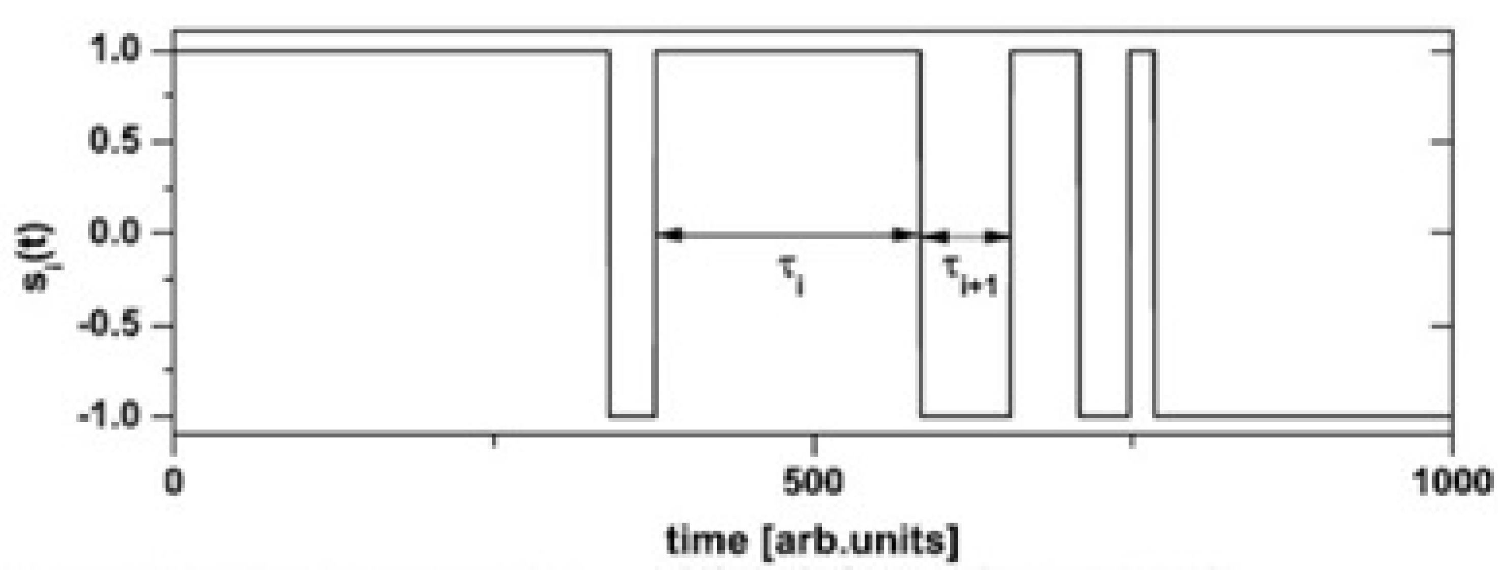
- The time series is composed of discrete events that are statistically independent of one another and are therefore renewal events (REs).
- (2)
- The time intervals between successive REs are described by an IPL PDF () and therefore constitute CETS.
- (3)
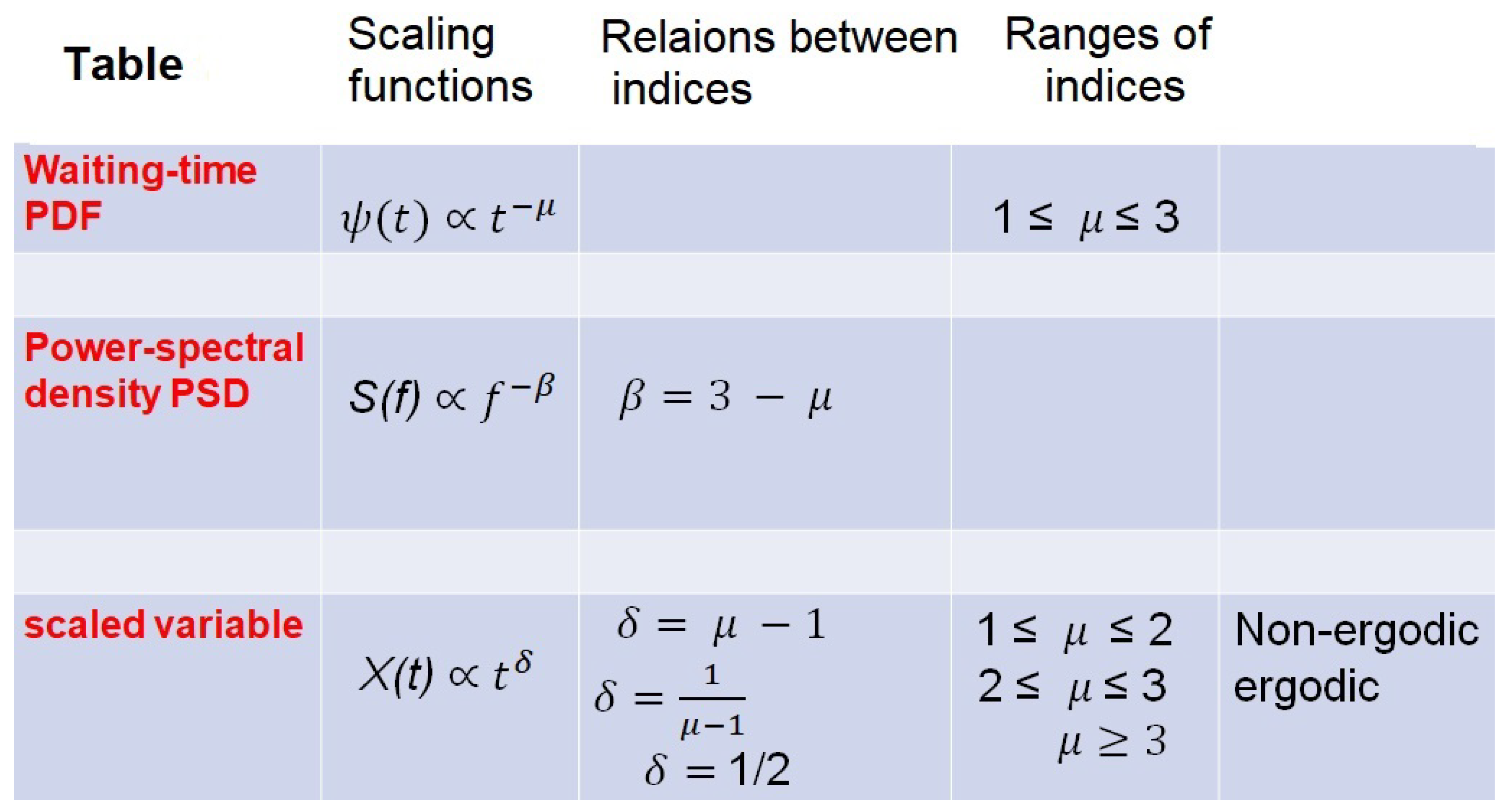
- The complexity of the CETS is measured by the MFD scaling index of the scaling PDF in phase to be (see SM1 for details involving the FOC).
- (4)
- The MFD is determined by the complexity of the time series in property 2 such that the MFD is equal to the IPL index , and the IPL index is related to the scaling index in property 3 by (see SM1 for details).
3. Formal Properties of CETS
3.1. Generating CETS
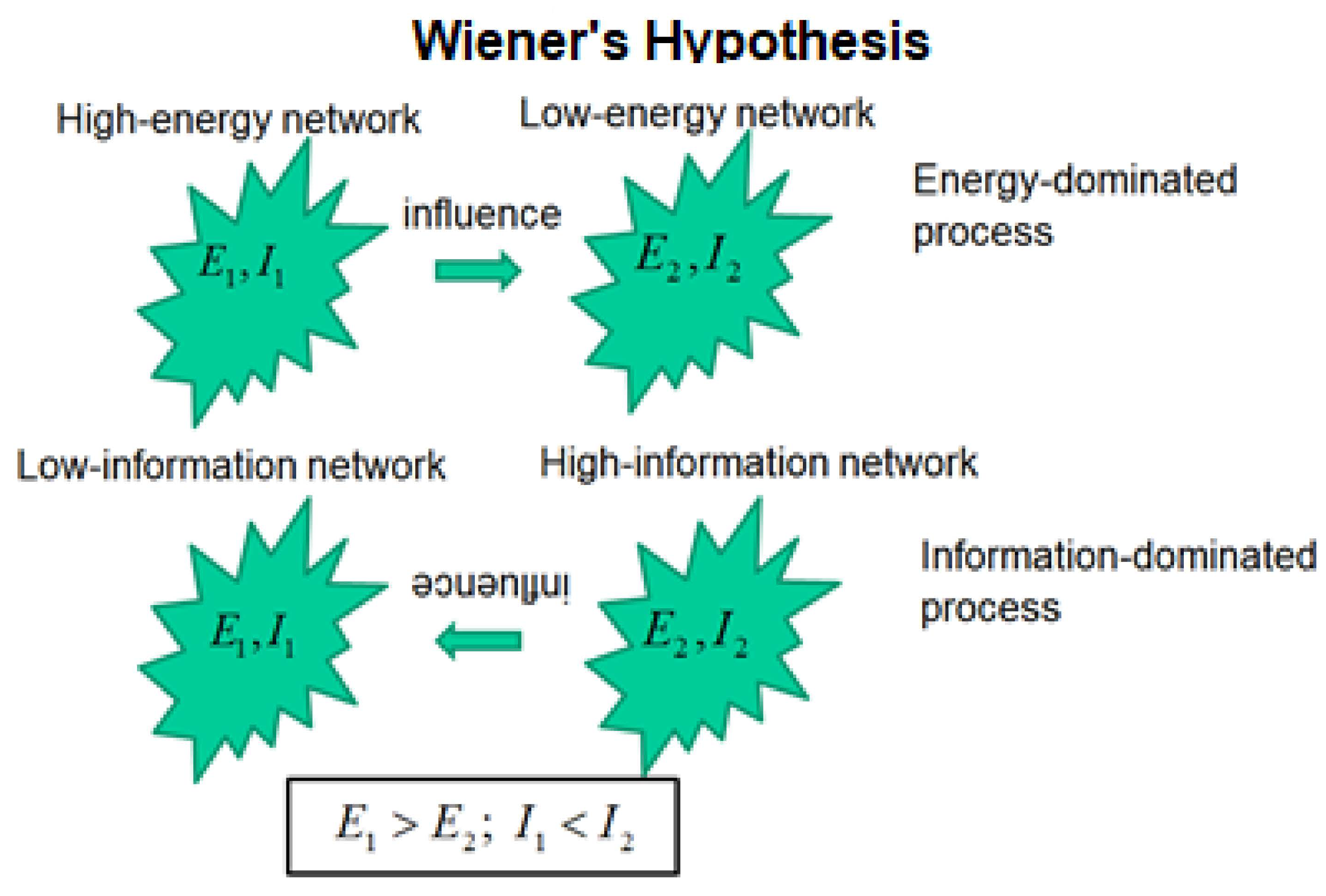
3.2. The Wiener Hypothesis
WH: Given the proper conditions, the force between two complex dynamic networks, produced by an energy gradient acting in one direction between the networks, can be overcome by the force produced by an information gradient acting in the opposite direction between the networks.
3.3. Information Exchange Between Networks
4. Detecting Empirical CEs in Datasets
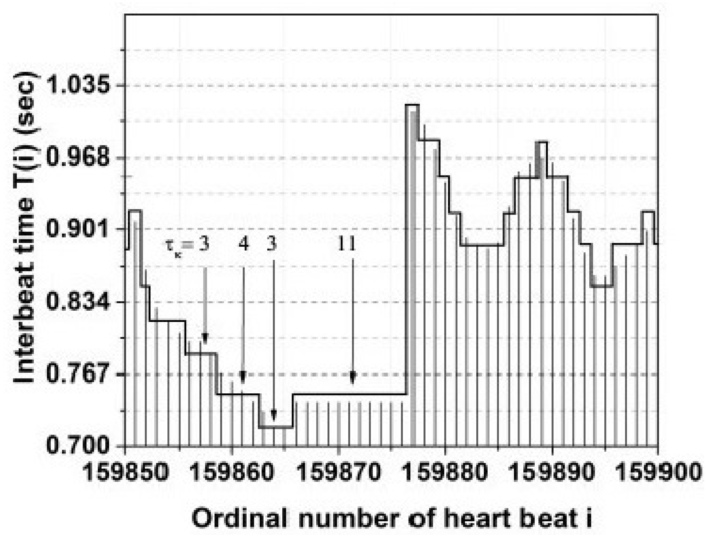
4.1. Heart Rate Variability (HRV)
4.2. Electroencephalograms (EEGs)
5. Complexity-Entailed Principles
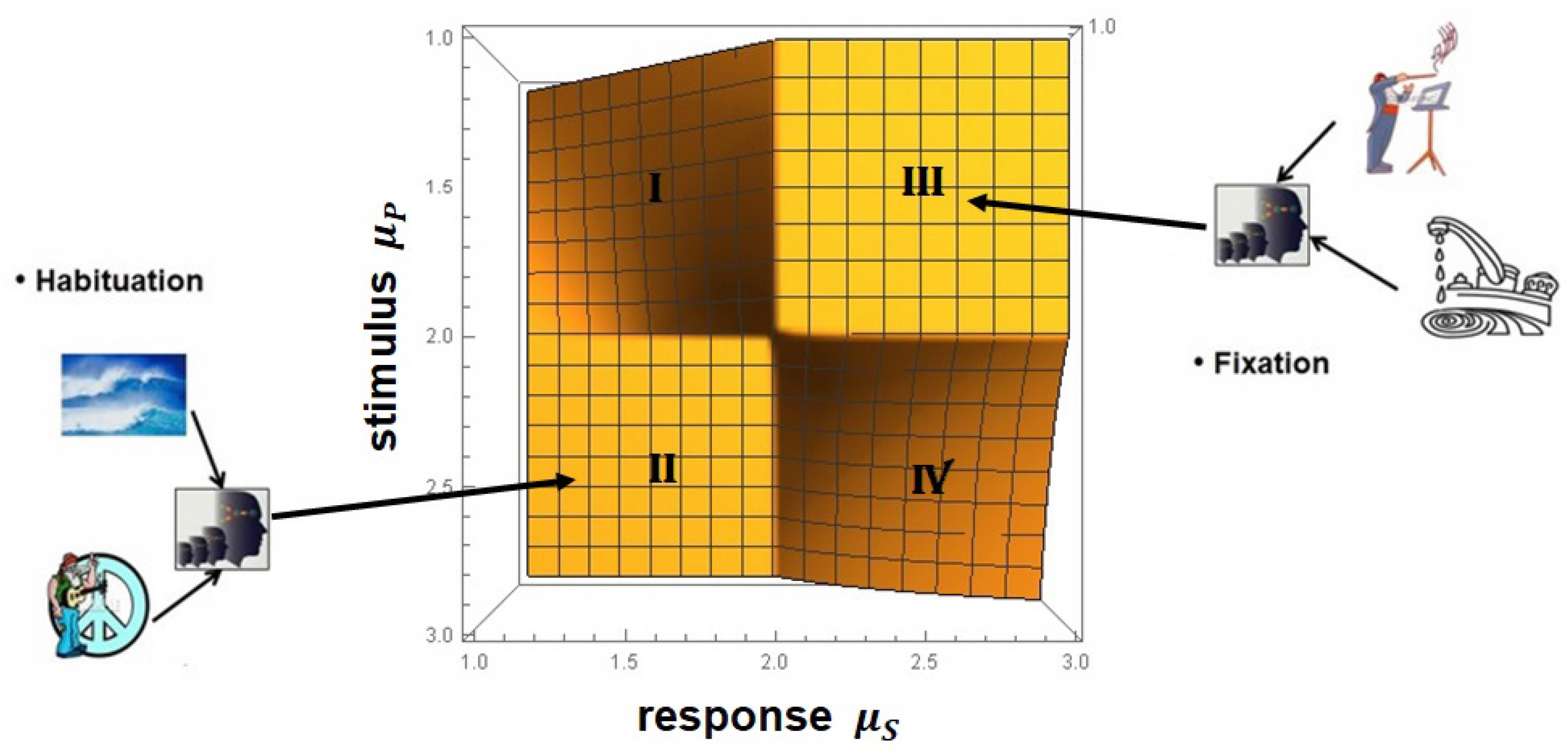
5.1. Principle of Complexity Matching and Management
- (1)
- A complex network belonging to ergodic region cannot exert any influence asymptotically on a second complex network belonging to non-ergodic region.
- (2)
- A complex network belonging to ergodic region exerts varying degrees of influence on a second complex network belonging to ergodic region. This follows from the PCM.
- (3)
- A complex network belonging to no-ergodic region exerts varying degrees of influence on a second complex network belonging to no-ergodic region. This follows from the PCM.
- (4)
- A complex network belonging to non-ergodic region transmits its full complexity to a second complex network belong to ergodic region, which was anticipated by the WH.
5.2. Memory and Generation Rate of CEs
5.3. MDEA Reveals Invisible CEs
5.4. Principle of Complexity Synchronization (CS)
6. Discussion
7. Conclusions
- (1)
- CEs are manifestations of cooperative interactions between the units of an ON that lead to a spontaneous self-organizing process, and for the life-sustaining networks considered herein, these are spontaeously generated by SOTC [16].
- (2)
- (3)
- The CCC shows that the demise of LRT only occurs asymptotically in a restricted domain of an ergodic ON stimulating a nonergodic ON.
- (4)
- The CCC shows that the WH is valid asymptotically in a restricted domain of a nonergodic ON stimulating a responding ergodic ON.
- (5)
- (6)
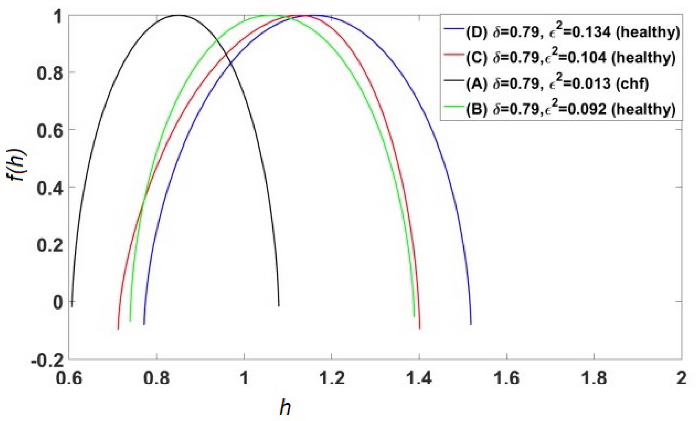
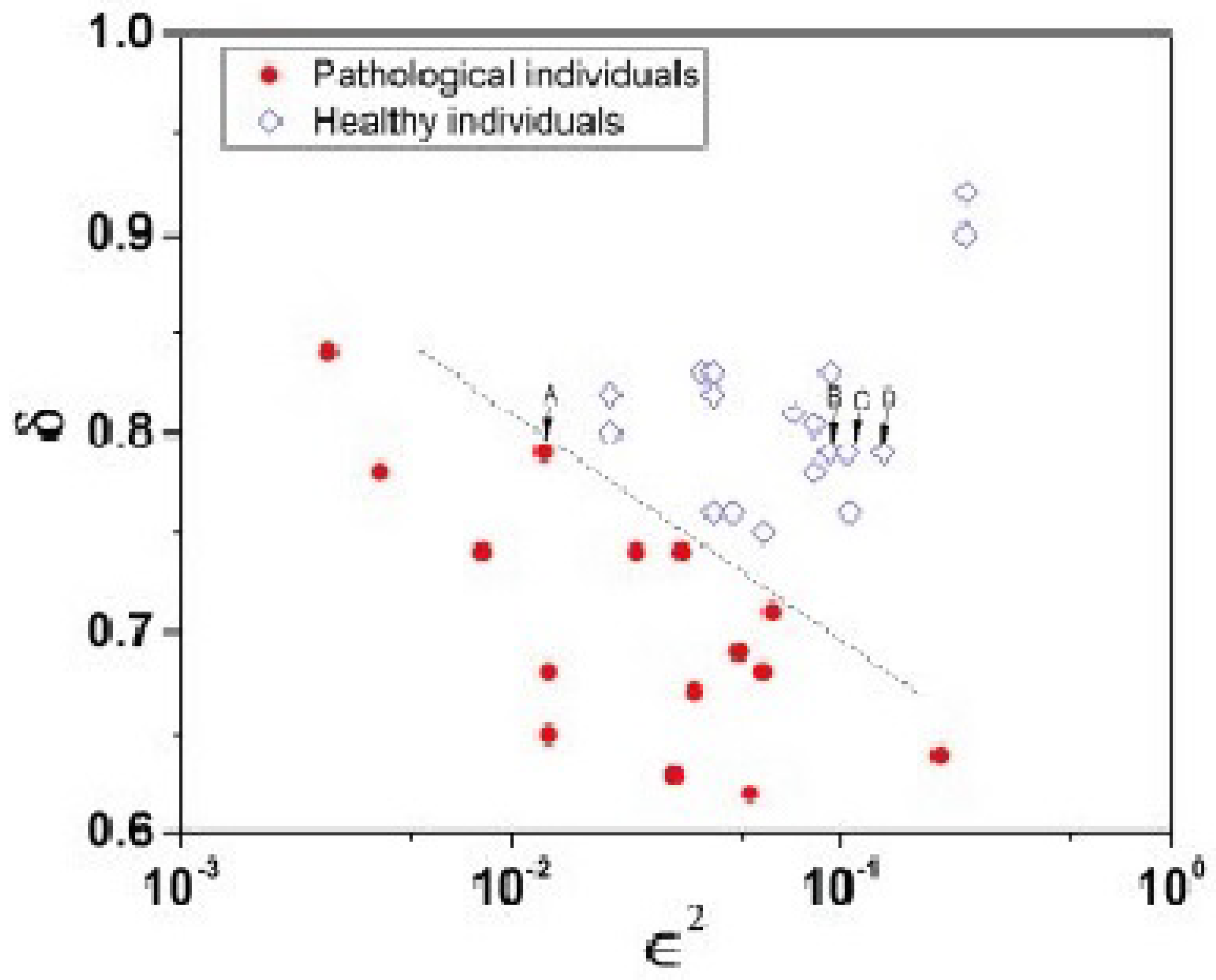
- The PCM&M has been empirically verified using MDEA to generate and the MFDS to generate , which is the probability that an event is crucial, thereby locating an individual on the ()-plane. This method partitions healthy and pathological subjects in this parameter space by applying the insights gained from the CCC to empirical ECG time series [62,91].
- (7)
- The MFD spectrum for healthy patients is broader than those with an illness or injury [17].
- (8)
- (9)
- (10)
- The new form of synchronization which we dubbed CS and which has been empirically determined [1,2,51] could just as easily have been called ‘multifractal dimension synchronization’ (MFDS) after the measure of complexity which manifests synchronization. It also suggests that if an ON is found having a different measure of complexity, we would expect the new measure to synchronize in accordance with the principle that optimizes the information exchange during an interacton.
Key Principle: Information Flow Is Physical and Measurable
- Assme all PTS are generated by a system that has multiscale memory until explicitly proven otherwise.
- This reinforces the role that non-Gaussian processes, which is to say CEs with IPL PDFs, play in generating PTS.
Supplementary Materials
Funding
Conflicts of Interest
Nomenclature
| AFBM | aging FBM |
| BRV | breath rate variability |
| CAN | cardiac autonomic neuorpathy |
| CE | crucial event |
| CETS | CE time series |
| CCC | cross-correlation cube |
| CME | complexity matching effect |
| CS | complexity synchronization |
| CSH | CS hypothesis |
| DEA | diffusion entropy analysis |
| EEG | electroencephlogram |
| ECG | electracaediogram |
| FA | fractal architecture |
| FAH | FA hypothesis |
| FBM | fractional Brownian motion |
| FDE | fractional diffusion equaton |
| FFPE | fractional Fokker–Planck equation |
| FKE | fractional kinetic equaition |
| FRW | fractal RW |
| FOC | fractional-order calculus |
| FOPC | FO probability calculus |
| HBL | heart, brain, lungs |
| HRV | heartrate variability |
| HTD | heavy-tailed distribution |
| IF | information force |
| IOC | integer-order calculus |
| IOPC | IO probability calclus |
| IPL | inverse power law |
| lT | Information Theory |
| LRT | linear response theory |
| MFD | multifractal dimension |
| MFDTS | MFD time sries |
| MFDS | MFD synchronization |
| MDEA | modified DEA |
| MFSA | multifractal signal analysis |
| MLF | Mittag–Leffler function |
| MODS | Multiple Organ Dysfunction Syndrome |
| MSE | multiscale entropy |
| NoONs | network of ONs |
| ON | organ network |
| PCM | principle of compexity matching |
| PCM&M | PCM and management |
| PFA | principle of FA |
| PMFDS | principle of MFDS |
| PD | Parkinson’s disease |
| probability density function | |
| PSD | power spectral density |
| PTS | physiological time series |
| RE | renewal event |
| RG | renormalization group |
| RW | random walk |
| SCPG | super central pattern generator |
| SHM | statistical habituation model |
| SFLE | simplest fractional Langevin equation |
| SM | supplementary material |
| SOC | self-organized criticality |
| SOTC | self-organized temporal criticality |
| SRV | stride rate variabilty |
| STEM | science technology engineering mathematics |
| WG | West/Grigolini |
| WH | Wiener hypothesis |
| WS | Wiener/Shannon |
References
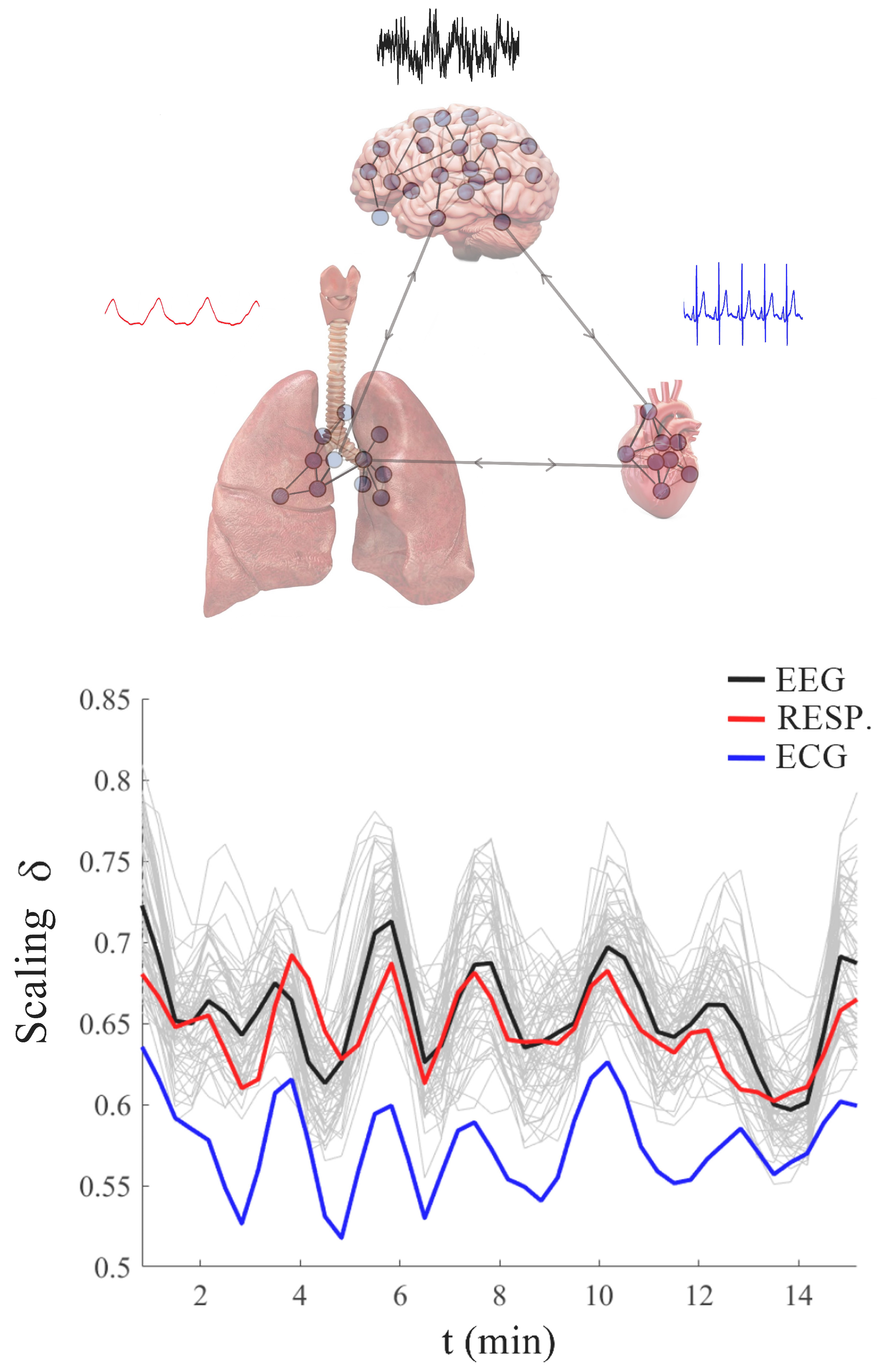
- Mahmoodi, K.; Kerick, S.E.; Grigolini, P.; Franaszczuk, P.J.; West, B.J. Complexity synchronization: A measure of interaction between the brain, heart and lungs. Sci. Rep. 2023, 13, 1143. [Google Scholar] [CrossRef] [PubMed]
- West, B.J.; Grigolini, P.; Kerick, S.E.; Franaszczuk, P.J.; Mahmoodi, K. Complexity synchronization of organ networks. Entropy 2023, 25, 1393. [Google Scholar] [CrossRef] [PubMed]
- Thurner, S. (Ed.) 43 Visions for Complexity; World Scientific: Singapore, 2017. [Google Scholar]
- West, B.J. Coloquium: Fractional calculus view of complexity: A tutorial. Rev. Mod. Phys. 2014, 86, 11691184. [Google Scholar] [CrossRef]
- West, B.J. (Ed.) Fractional Calculus and the Future of Science; Special Issue of Entropy; MDPI: Basel, Switzerland, 2022. [Google Scholar]
- Buzsáki, G. The Brain from Inside Out; Oxford University Press: Oxford, NY, USA, 2019. [Google Scholar]
- Songe, F.; Karniadakis, G.E. Variable-Order Fractional Models for Wall-Bounded Turbulent Flows. Entropy 2021, 23, 782. [Google Scholar] [CrossRef]
- Beggs, J.; Plenz, I. Neuronal avalanches in neocortical circuits. J. Neurosci. 2003, 23, 11.167–11.177. [Google Scholar] [CrossRef]
- West, B.J.; Grigolini, P. Habituation and 1/f-noise. Physica A 2010, 389, 5706. [Google Scholar] [CrossRef]
- Turalska, M.; West, B.J. Fractional dynamics of individuals in complex networks. Front. Physiol. 2018, 6, 110. [Google Scholar] [CrossRef]
- West, B.J.; Grigolini, P. Crucial Events; Why Are Catastrophes Never Expected? Studies of Nonlinear Phenomena in Life Science; World Scientific: Hackensack, NJ, USA, 2021; Volume 17. [Google Scholar]
- Wiener, N. Cybernetics; MIT Press: Cambridge, MA, USA, 1948. [Google Scholar]
- Shannon, C.E. A Mathematical Theory of Communication. Bell Sys. Tech. J. 1948, 27, 379–423, IBID 623–656. [Google Scholar] [CrossRef]
- Wiener, N. The Human Use of Human Beings; Da Capo: Avon, NY, USA, 1950. [Google Scholar]
- Ashby, W.R. An Introduction to Cybernetics; Chapman & Hall Ltd.: London, UK, 1957. [Google Scholar]
- Mahmoodi, K.; West, B.J.; Grigolini, P. Self-Organizing Complex Networks: Individual versus global rules. Front. Physiol. 2017, 8, 478. [Google Scholar] [CrossRef]
- West, B.J.; Geneston, E.L.; Grigolini, P. Maximizing information exchange between complex networks. Phys. Rep. 2008, 468, 1–99. [Google Scholar] [CrossRef]
- Aquino, G.; Bologna, M.; Grigolini, P.; West, B.J. Transmission of information between complex systems: 1/f resonance. Phys. Rev. E 2011, 83, 051130. [Google Scholar] [CrossRef] [PubMed]
- Abney, D.H.; Paxton, A.; Dale, R.; Kello, C.T. Complexity matching of dyadic conversation. J. Exp. Psychol. Gen. 2014, 143, 2304. [Google Scholar] [CrossRef] [PubMed]
- Almurad, Z.M.H.; Roume, C.; Delignières, D. Complexity matching in side-byside walking. Hum. Mov. Sci. 2017, 54, 125. [Google Scholar] [CrossRef] [PubMed]
- Almurad, Z.M.H.; Roume, C.; Delignières, D. Complexity Matching: Restoring the Complexity of Locomotion in Older People Through Arm-in-Arm Walking. Front. Physiol. Fractal Physiol. 2018, 10, 3389. [Google Scholar] [CrossRef]
- Coey, C.A.; Washburn, A.; Hassebrock, J.; Richardson, M.J. Complexity matching effects in bimanual and interpersonal syncopated finger tapping. Neurosci. Lett. 2016, 616, 204. [Google Scholar] [CrossRef]
- Deligniéres, D.; Almurad, Z.M.H.; Roume, C.; Marmelat, V. Multifractal signatures of complexity matching. Exp. Brain Res. 2016, 234, 2773. [Google Scholar] [CrossRef]
- Fine, J.M.; Likens, A.D.; Amazeen, E.L.; Amazeen, P.G. Emergent Complexity Matching in Interpersonal Coordination: Local Dynamics and Global Variability. J. Exp. Psych. Hum. Percept. Perform. 2015, 41, 723. [Google Scholar] [CrossRef]
- Marmelat, V.; Deligniéres, D.D. Strong anticipation: Complexity matching in interpersonal coordination. Exp. Brain. Res. 2012, 222, 137. [Google Scholar] [CrossRef]
- Shannon, C.E.; Weaver, W. The Mathematical Theory of Communication; The University of Illinois Press: Urbana, IL, USA, 1949. [Google Scholar]
- von Neumann, J. The Computer and the Brain; Yale University Press: New Haven, CT, USA, 1958. [Google Scholar]
- Mandelbrot, B.B. Fractals: Form, Chance and Dimension; W.H. Freeman and Co.: San Francisco, CA, USA, 1977. [Google Scholar]
- West, B.J.; Goldberger, A. Physology in Fractal Dimensions. Am. Sci. 1987, 75, 354–365. [Google Scholar]
- Shlesinger, M.F. Fractal time and 1/f-noise in complex systems. Ann. N. Y. Acad. Sci. 1987, 504, 214–228. [Google Scholar] [CrossRef]
- Goldberger, A.L.; West, B.J. Fractals in Physiology and Medicine. Yale J. Biol. Med. 1987, 60, 421–435. [Google Scholar] [PubMed]
- West, B.J. Fractals, Intermittency and Morphogenesis. In Chaos in Biological Systems; Degn, H., Holden, A.V., Olsen, L.F., Eds.; Plenum Publishing Corporation: Washington, DC, USA, 1987. [Google Scholar]
- West, B.J. Fractal physiology: A paradigm for adaptive response. In Dynamic Patterns in Complex Systems; Kelso, J.A.S., Mandell, A.J., Shlesinger, M.F., Eds.; World Science: Singapore, 1988. [Google Scholar]
- West, B.J. Physiology in Fractal Dimensions: Error Tolerance. Ann. Biomed. Eng. 1990, 18, 135–149. [Google Scholar] [CrossRef] [PubMed]
- Buzsáki, G. Rhythms of the Brain; Oxford University Press: Oxford, NY, USA, 2006. [Google Scholar]
- Lashley, K.S. Mass action and cerebral function. Science 1931, 73, 245–254. [Google Scholar] [CrossRef] [PubMed]
- Salingaros, N.A.; West, B.J. A Universal Rule for the Distribution of Sizes. Environ. Plan. Urban Anal. City Sci. 1999, 26, 909–923. [Google Scholar] [CrossRef]
- Barthelemy, M. The Statistical Physics of Cities. Nat. Rev. Phys. 2019, 1, 406–415. [Google Scholar] [CrossRef]
- Molinero, C. A Fractal Theory of Urban Growth. Front. Front. Phys. Sec. Soc. Phys. 2022, 10, 861678. [Google Scholar] [CrossRef]
- West, G.B.; Brown, J.; Enquist, B.J. The Fourth Dimension of Life: Fractal Geometry and Allometric Scaling of Organisms. Science 1999, 284, 1677–1679. [Google Scholar] [CrossRef]
- Singer, W. Consciousness and neuronal synchronization. In The Consciousness; Tononi, G., Laureys, S., Eds.; Academic Press: Cambridge, MA, USA, 2021. [Google Scholar]
- Bassingthwaighte, J.B.; Liebovitch, L.S.; West, B.J. Fractal Physiology; Oxford University Press: Oxford, UK, 1994. [Google Scholar]
- West, B.J.; Deering, W. Fractal physiology for physicists: Levy statistics. Phys. Rep. 1994, 246, 1–100. [Google Scholar] [CrossRef]
- Nonnenmacher, T.F.; Losa, G.A.; Weibel, E.R. Fractals in Biology and Medicine; Birkhäuser: Basel, Switzerland, 2013. [Google Scholar]
- Weibel, E.R. Symmorphosis, On Form and Function in Shaping Life; Harvard University Press: Cambridge, MA, USA, 2000. [Google Scholar]
- West, B.J.; Grigolini, P.; Bologna, M. Crucial Event Rehabilitation Therapy: Multifractal Medicine; Springer International Publishing: Berlin/Heidelberg, Germany, 2024. [Google Scholar]
- Zaslavsky, G.M. Hamiltonian Chaos & Fractional Dynamics; Oxford University Press: Oxford, UK, 2005. [Google Scholar]
- Feller, W. Intoduction to Probability Theory and Its Applications; J. Wiley & Sons: New York, NY, USA, 1991; Volume 2. [Google Scholar]
- Cox, D.R. Renewal Theory; Metheum & Co.: London, UK, 1967. [Google Scholar]
- Feder, J. Fractals; Plenum Press: New York, NY, USA, 1988. [Google Scholar]
- Mahmoodi, K.; Kerick, S.E.; Grigolini, P.; Franaszczuk, P.J.; West, B.J. Temporal complexity measure of reaction time series: Operational versus event time. Brain Behav. 2023, 13, e3069. [Google Scholar] [CrossRef]
- Korolj, A.; Wu, H.; Radisic, M. A healthy dose of chaos: Using fractal frameworks for engineering higher-fidelity biomedical systems. Biomaterials 2019, 219, 119363. [Google Scholar] [CrossRef]
- West, B.J.; Mutch, W.A.C. On the Fractal Language of Medicne; FOT4STEM; CRC Press: Boca Raton, FL, USA, 2024; Volume 2. [Google Scholar]
- Mega, M.S.; Allegrini, P.; Grigolini, P.; Latora, V.; Palatella, L.; Rapisarda, A.; Palatella, L. Power-Law Time Distribution of Large Earthquakes. Phys. Rev. Lett. 2003, 90, 188501. [Google Scholar] [CrossRef] [PubMed]
- West, B.J. Where Medicine Went Wrong; Studies in Nonlinear Phenomena in Life Science; World Scientific: Hackensack, NJ, USA, 2006; Volume 11. [Google Scholar]
- Allegrini, P.; Fronzoni, L.; Grigolini, P.; Latora, V.; Mega, M.S.; Palatella, L.; Rapisarda, A.; Vinciguerra, S. Detection of invisible and crucial events: From seismic fluctuations to the war against terrorism. Chaos Solitons Fractals 2004, 20, 77–85. [Google Scholar] [CrossRef]
- Feller, W. Fluctuation theory of recurrent events. Trans. Am. Math. Soc. 1949, 67, 98. [Google Scholar] [CrossRef]
- Efros, A.L.; Nesbitt, D.J. Origin and control of blinking in quantum dots. Nat. Nanotechnol. 2016, 11, 661–671. [Google Scholar] [CrossRef]
- Narumi, T.; Mikami, Y.; Nagaya, T.; Okabe, H.; Hara, K.; Hidaka, Y. Relaxation with long-period oscillation in defect turbulence of planar nematic liquid crystals. Phys. Rev. E 2016, 94, 042701. [Google Scholar] [CrossRef]
- Bak, P.; Tang, C.; Wiesenfeld, K. Self-organized criticality: An explanation of 1/f noise. Phys. Rev. Lett. 1987, 59, 381. [Google Scholar] [CrossRef]
- Lipiello, E.; Arcangelis, L.D.; Godano, C. Memory in self-organized criticality. Europhys. Lett. 2005, 72, 678. [Google Scholar] [CrossRef]
- Allegrini, P.; Grigolini, P.; Hamilton, P.; Palatella, L.; Raffaelli, G. Memory beyond memory in heart beating, a sign of a healthy physiological condition. Phys. Rev. E 2002, 65, 041926. [Google Scholar] [CrossRef]
- Barenblatt, G.I. Scaling, Self-Similarity, and Intermediate Asymptotics; Cambridge Texts in Applied Mathematics 14; Cambridge University Press: Cambridge, UK, 1996. [Google Scholar]
- Peng, C.-K.; Mietus, J.; Hausdorff, J.M.; Havlin, S.; Stanley, H.G.; Goldberger, A.L. Long-range anticorrelations and non-Gaussian behavior of the heartbeat. Phys. Rev. Lett. 1993, 70, 1343. [Google Scholar] [CrossRef]
- Peng, C.-K.; Mietus, J.E.; Liu, Y.; Khalsa, G.; Douglas, P.S.; Benson, H.; Goldberger, A.L. Exaggerated heart rate oscillations during two meditation techniques. Int. J. Cardiol. 1999, 70, 101–107. [Google Scholar] [CrossRef]
- West, B.J. Complexity synchronization in living matter: A mini review. Front. Netw. Physiol. 2024, 4, 1379892. [Google Scholar] [CrossRef] [PubMed]
- Scafetta, N.; Grigolini, P. Scaling detection in time series: Diffusion Entropy Analysis. Phys. Rev. E 2002, 66, 036130. [Google Scholar] [CrossRef] [PubMed]
- Goldberger, A.L.; Rigney, D.R.; West, B.J. Chaos and fractals in humaan physiology. Sci. Am. 1990, 262, 42–49. [Google Scholar] [CrossRef] [PubMed]
- Goldberger, A.L. Nonlinear dynamics for clinicians: Chaos theory, fractals, and complexity at the bedside. Lancet 1996, 347, 1312–1314. [Google Scholar] [CrossRef]
- West, B.J. Fractal Calculus Facilitates Rethinking ‘Hard Problems’; A New Research Paradigm. Fractal Fract. 2024, 8, 620. [Google Scholar] [CrossRef]
- Paradisi, P.; Cesari, R.; Donateo, A.; Contini, D.; Allegrini, P. Diffusion scaling in event-driven random walks: An applicatiion to turbulence. Rept. Math. Phys. 2012, 70, 205–220. [Google Scholar] [CrossRef]
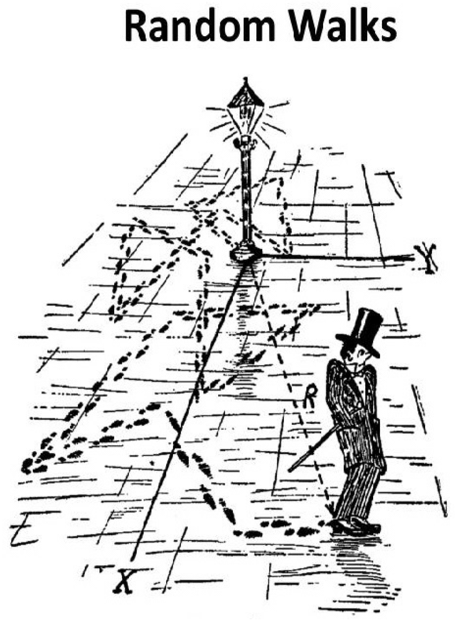
- Rayleigh, L. The problem of the random walk. Nature 1905, 72, 318. [Google Scholar] [CrossRef]
- Einstein, A. ber die von der molekularkinetischen Theorie der W rme geforderte Bewegung von in ruhenden Fl ssigkeiten suspendierten Teilchen. Ann. Phys. 1905, 322, 549–560. [Google Scholar] [CrossRef]
- Gamow, G. One, Two, Three...Infinity; The Viking Press: New York, NY, USA, 1947. [Google Scholar]
- Carroll, L. Through the Looking Glass; Macmillan: London, UK, 1871. [Google Scholar]
- Hosking, J.T.M. Fractional Differencing. Biometrika 1981, 88, 165–176. [Google Scholar] [CrossRef]
- West, B.J. Physiology, Promiscuity and Prophecy at the Millennium: A Tale of Tails; Studies of Nonlinear Phenomena in Life Science 7; World Scientific: Hackensack, NJ, USA, 1999. [Google Scholar]
- Mandelbrot, B.B.; Van Ness, J.W. Fractional Brownian motion, fractional noises and applications. SIAM Rev. 1968, 10, 422–437. [Google Scholar] [CrossRef]
- Mannella, R.; Grigolini, P.; West, B.J. A dynamical approach to fractional Brownian motion. Fractals 1994, 2, 81–94. [Google Scholar] [CrossRef]
- Culbreth, G.; West, B.J.; Grigolini, P. Entropic Approach to the Detection of Crucial Events. Entropy 2019, 21, 178. [Google Scholar] [CrossRef] [PubMed]
- Kolmogorov, A.N. Wienersche spiralen und einige andere interessante Kurven im Hilbertschen Raum, C.R. (doklady). Acad. Sci. URSS (N.S.) 1940, 26, 115–118. [Google Scholar]
- Taqqu Benoît, M.S. Mandelbrot and Fractional Brownian Motion. Stat. Sci. 2013, 28, 131–134. [Google Scholar]
- Deligniéres, D.; Lemoine, L.; Torre, K. Time intervals production in tapping and oscillatory motion. Hum. Mov. Sci. 2004, 23, 87–103. [Google Scholar] [CrossRef]
- Deligniéres, D.; Torre, K.; Lemoine, L. Fractal models for event-based and dynamical timers. Acta Psychol. 2008, 127, 382–397. [Google Scholar] [CrossRef]
- Vierordt, K. Über das Gehen des Menchen in Gesunden und Kranken Zus Taenden nach Selbstregistrirender Methoden; Laupp: Tuebigen, Germany, 1881. [Google Scholar]
- Hausdorff, J.M.; Peng, C.K.; Ladin, Z.; Wei, J.Y.; Goldberger, A.L. Is walking a random walk? Evidence for long-range correlations in stride interval of human gait. J. Appl. Physiol. 1995, 78, 349–358. [Google Scholar] [CrossRef]
- Deligniéres, D.; Torre, K. Fractal dynamics of human gait: A reassessment of the 1996 data of Hausdorff et al. J. Appl. Physiol. 2009, 106, 1272–1279. [Google Scholar] [CrossRef]
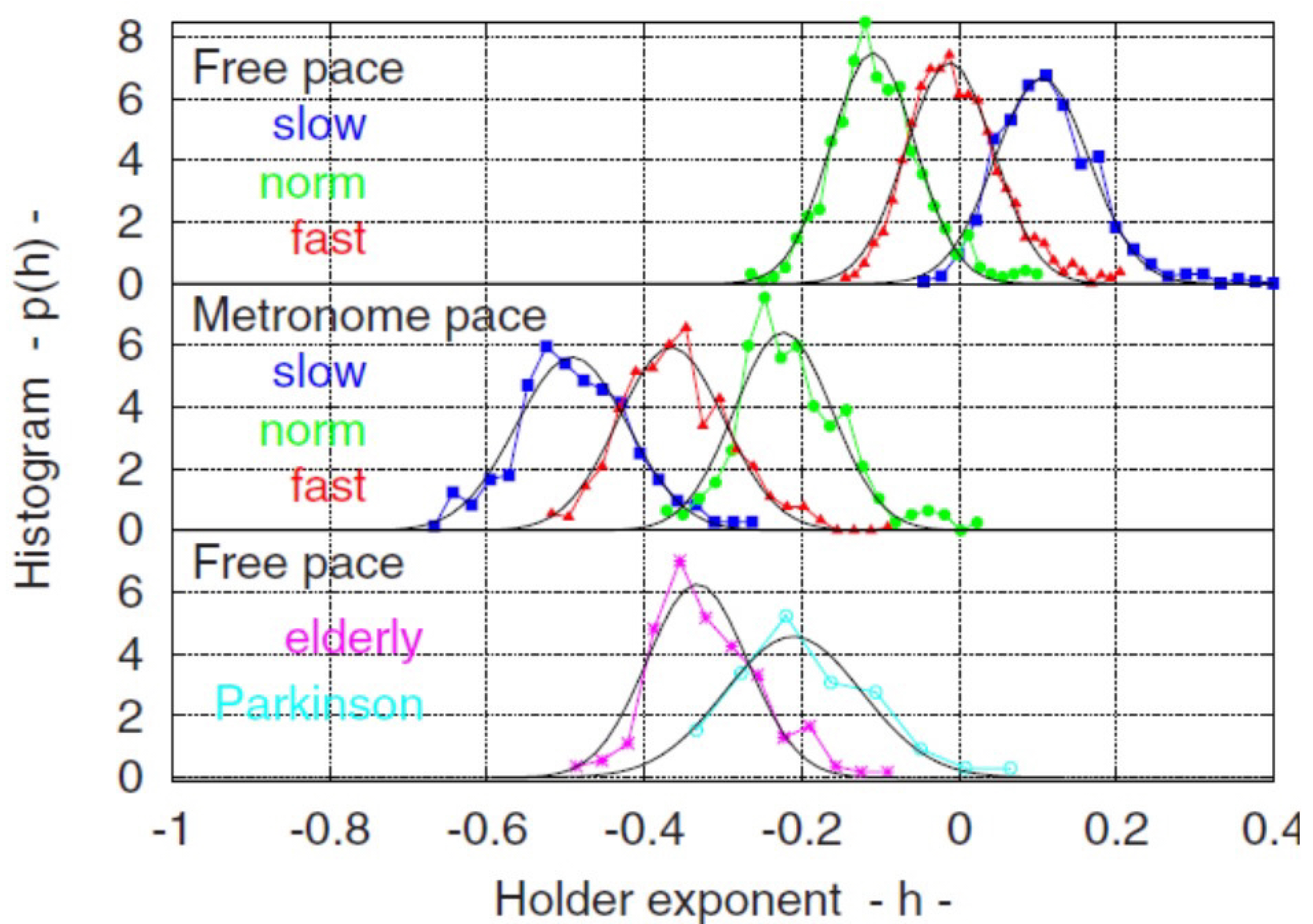
- Scafetta, N.; Marchi, D.; West, B.J. Understanding the complexity of human gait dynamics. Chaos 2009, 19, 026108. [Google Scholar] [CrossRef]
- West, B.J.; Scafetta, N. A nonlinear model for human gait. Phys. Rev. E 2003, 67, 051917. [Google Scholar] [CrossRef]
- Ivanov, P.C.; Amaral, L.A.N.; Goldberger, A.L.; Havlin, S.; Rosenblum, M.G.; Struzikk, Z.R.; Stanley, H.E. Multifractality in human heartbeat dynamics. Nature 1999, 399, 461. [Google Scholar] [CrossRef] [PubMed]
- Bohara, G.; Lambert, D.; West, B.J.; Grigolini, P. Crucial events, randomness and multi-fractality in heartbeats. Phys. Rev. E 2017, 96, 06216. [Google Scholar] [CrossRef] [PubMed]
- West, B.J. Control from an Allometric perspective. In Progress in Motor Control; Sternad, D., Ed.; Advances in Experimental Medicine and Biology; Springer: Berlin/Heidelberg, Germany, 2009; pp. 57–82. [Google Scholar]
- Barkai, E.; Garini, Y.; Metzler, R. Strange kinetics of single molecules in living cells. Phys. Today 2012, 65, 29. [Google Scholar] [CrossRef]
- Jelinek, H.F.; Tuladhar, R.; Culbreth, G.; Bohara, G.; Cornforth, D.; West, B.J.; Grigolini, P. Diffusion Entropy vs. Multiscale and Rényi Entropy to Detect Progression of Autonomic Neuropathy. Front. Physiol. 2021, 11, 607324. [Google Scholar] [CrossRef]
- Baxley, J.D.; Lambert, D.R.; Bologna, M.; West, B.J.; Grigolini, P. Unveiling Pseudo-Crucial Events in Noise-Induced Phase Transitions. Chaos Solitons Fractals 2023, 172, 113580. [Google Scholar] [CrossRef]
- Bettencourt, L.A.; Ulwick, A.W. The customer-centered innovation map. Harv. Bus. Rev. 2008, 86, 109. [Google Scholar]
- Mahmoodi, K.; West, B.J.; Grigolini, P. Self-Organized Temporal Criticality: Bottom-Up Resilience versus Top-Down Vulnerability. Complexity 2018, 2018, 8139058. [Google Scholar] [CrossRef]
- Stanley, H.G. Introduction to Phase Transitions and Critical Phenomena; Oxford University Press: New York, NY, USA; Oxford, UK, 1971. [Google Scholar]
- West, B.J. Information force. J. Theor. Comp. Sci. 2016, 3, 144. [Google Scholar] [CrossRef]
- Wiener, N. Time, Communication and the Nervous System. Proc. N. Y. Acad. Sci. 1948, 50, 197–220. [Google Scholar] [CrossRef]
- Schrödinger, E. What Is Life? The Physical Aspect of the Living Cell; First Pub. 1944; Cambridge University Press: Cambridge, UK, 1967. [Google Scholar]
- Kello, C.T.; Beltz, B.C.; Holden, J.G.; Van Orden, G.C. The Emergent Coordination of Cognitive Function. J. Exp. Psych. 2007, 136, 551. [Google Scholar] [CrossRef]
- Pease, A.; Mahmoodi, K.; West, B.J. Complexity measures of music. Chaos Solitons Fractals 2018, 108, 82. [Google Scholar] [CrossRef]
- Su, Z.-Y.; Wu, T. Music walk, fractal geometry in music. Physica A 2007, 380, 418. [Google Scholar] [CrossRef]
- Voss, R.F.; Clarke, J. ‘1/f-noise’ in music and speech. Nature 1975, 258, 317. [Google Scholar] [CrossRef]
- Li, W.; Holste, D. Universal 1/f noise, crossovers of scaling exponents, and chromosome-specific patterns of guaninecytosine content in DNA sequences of the human genome. Phys. Rev. E 2005, 71, 041910. [Google Scholar] [CrossRef]
- Sumpter, D.J.T. The principles of collective animal behaviour. Phil. Trans. R. Soc. B 2006, 361, 5. [Google Scholar] [CrossRef]
- Tuladhar, R.; Bohara, G.; Grigolini, P.; West, B.J. Meditation-induced coherence and crucial events. Front. Physiol. 2018, 9, 626. [Google Scholar] [CrossRef]
- Bohara, G.; West, B.J.; Grigolini, P. Bridging waves and crucal events in the dynamics of the brain. Front. Physiol. 2018, 9, 1174. [Google Scholar] [CrossRef]
- Barbi, E.; Bologna, M.; Grigolini, P. Linear Response to Perturbation of Non-exponential Renewal Processes. Phys. Rev. Lett. 2005, 95, 220601. [Google Scholar] [CrossRef]
- Heinsalu, E.; Patriarca, M.; Goychuk, I.; Hänggi, P. Use and Abuse of a Fractional Fokker-Planck Dynamics for Time-Dependent Driving. Phys. Rev. Lett. 2007, 99, 120602. [Google Scholar] [CrossRef]
- Magdziarz, M.; Weon, A.; Klafter, J. Equivalence of the Fractional Fokker-Planck and Subordinated Langevin Equations: The Case of a Time-Dependent Force. Phys. Rev. Lett. 2008, 101, 210601. [Google Scholar] [CrossRef]
- Shushin, A.I. Effect of a time-dependent field on subdiffusing particles. Phys. Rev. E 2008, 78, 051121. [Google Scholar] [CrossRef] [PubMed]
- Sokolov, I.M. Linear response to perturbation of non-exponential renewal process: A generalized master equation approach. Phys. Rev. E 2006, 73, 067102. [Google Scholar] [CrossRef] [PubMed]
- Weron, A.; Magdziarz, M.; Weron, K. Modeling of subdiffusion in space-time dependent force fields beyond the fractional Fokker-Planck equation. Phys. Rev. E 2008, 77, 036704. [Google Scholar] [CrossRef] [PubMed]
- Sokolov, I.M.; Blumen, A.; Klafter, J. Linear response in complex systems: CTRW and the fractional Fokker–Planck equations. Physica A 2001, 302, 268. [Google Scholar] [CrossRef]
- Aquino, G.; Bologna, M.; Grigolini, P.; West, B.J. Beyond the death of linear response theory: Criticality of the 1/-noise condition. Phys. Rev. Lett. 2010, 105, 040601. [Google Scholar] [CrossRef]
- Kubo, R.; Toda, M.; Hashitusume, N. Statistical Physics; Springer: Berlin, Germany, 1985. [Google Scholar]
- Piccinini, N.; Lambert, D.; West, B.J.; Bologna, M.; Grigolini, P. Nonergodic Complexity Management. Phys. Rev. E 2016, 93, 062301. [Google Scholar] [CrossRef]
- Wang, D. Habituation. In Handbook of Brain Theory and Neural Networks; Arbib, M.A., Ed.; MIT Press: Cambridge, MA, USA, 1995; p. 441. [Google Scholar]
- Penna, T.J.P.; de Oliveira, P.M.C.; Sartorelli, J.C.; Goncalves, W.M.; Pinto, R.D. Long-range anti-correlation and non-Gaussian behavior of a leaky faucet. Phys. Rev. E 1995, 52, R2168–R2171. [Google Scholar] [CrossRef]
- Allegrini, P.; Menicucci, D.; Bedini, R.; Gemignani, A.; Paradisi, P. Complex intermittency blurred by noise: Theory and application to neural dynamics. Phys. Rev. E 2010, 82, 015103. [Google Scholar] [CrossRef]
- West, B.J.; Deering, W. The Lure of Modern Science; Studies in Nonlinear Phenomena in Life Science; World Scientific: Singapore, 1995; Volume 3. [Google Scholar]
- Allegrini, P.; Barbi, F.; Grigolini, P.; Paradisi, P. Aging and renewal events in spordically modulated systems. Chaos Solitons Fractals 2007, 34, 11–18. [Google Scholar] [CrossRef]
- Grigolini, P.; Palatella, L.; Raffaelli, G. Asymmetric Anomalous Diffusion: An Efficient Way to Detect Memory in Time Series. Fractals 2001, 9, 439–449. [Google Scholar] [CrossRef]
- Buchman, T.G. Physiologic stability and physiologic state. J. Trauma 1996, 41, 599–605. [Google Scholar] [CrossRef] [PubMed]
- Buchman, T.G. Physiologic Failure: Multiple Organ Dysfunction Syndrome. In Complex Systems Science in Biomedicine; Deisboeck, T.S., Kresh, J.Y., Eds.; Topics in Biomedical Engineering International Book Series; Springer: Boston, MA, USA, 2006; pp. 631–640. [Google Scholar]
- Goldberger, A.L.; Amaral, L.A.; Hausdorff, J.M.; Ivanov, P.; Peng, C.K.; Stanley, H.E. Fractal dynamics in physiology: Alterations with disease and aging. Proc. Natl. Acad. Sci. USA 2002, 99 (Suppl. S1), 2466–2472. [Google Scholar] [CrossRef] [PubMed]
- Boker, A.; Graham, M.R.; Walley, K.R.; McManus, B.M.; Girling, L.G.; Walker, E.; Lefevre, G.R.; Mutch, W.A. Improved arterial oxygenation with biologically variable or fractal ventilation using low tidal volumes in a porcine model of acute respiratory distress syndrome. Am. J. Respir. Crit. Care Med. 2002, 165, 456–462. [Google Scholar] [CrossRef] [PubMed]
- Boker, A.; Haberman, C.J.; Girling, L.; Guzman, R.P.; Louridas, G.; Tanner, J.R.; Cheang, M.; Maycher, B.W.; Bell, D.D.; Doak, G.J. Variable ventilation improves perioperative lung function in patients undergoing abdominal aortic aneurysmectomy. Anesthesiology 2004, 100, 608–616. [Google Scholar] [CrossRef]
- Brewster, J.F.; Graham, M.R.; Mutch, W.A. Convexity, Jensen’s inequality and benefits of noisy mechanical ventilation. J. R. Soc. Interface 2005, 2, 393–396. [Google Scholar] [CrossRef]
- Kowalski, S.; McMullen, M.C.; Girling, L.G.; McCarthy, B.G. Biologically variable ventilation in patients with acute lung injury: A pilot study. Can. J. Anaesth. 2013, 60, 502–503. [Google Scholar] [CrossRef]
- McMullen, M.C.; Girling, L.G.; Graham, M.R.; Mutch, W.A. Biologically variable ventilation improves oxygenation and respiratory mechanics during one-lung ventilation. Anesthesiology 2007, 105, 91–97. [Google Scholar] [CrossRef]
- Mutch, W.A.; Harms, S.; Lefevre, G.R.; Graham, M.R.; Girling, L.G.; Kowalski, S.E. Biologically variable ventilation increases arterial oxygenation over that seen with positive end-expiratory pressure alone in a porcine model of acute respiratory distress syndrome. Crit. Care Med. 2000, 28, 2457–2464. [Google Scholar] [CrossRef]
- Mutch, W.A.; Buchman, T.G.; Girling, L.G.; Walker, E.K.; McManus, B.M.; Graham, M.R. Biologically variable ventilation improves gas exchange and respiratory mechanics in a model of severe bronchospasm. Crit. Care Med. 2007, 35, 1749–1755. [Google Scholar] [CrossRef]
- Ivanov, P.C.; Liu, K.K.L.; Bartsch, R.P. Focus on the emerging new fields of network physiology and network medicine. New J. Phys. 2016, 18, 100201. [Google Scholar] [CrossRef]

Disclaimer/Publisher’s Note: The statements, opinions and data contained in all publications are solely those of the individual author(s) and contributor(s) and not of MDPI and/or the editor(s). MDPI and/or the editor(s) disclaim responsibility for any injury to people or property resulting from any ideas, methods, instructions or products referred to in the content. |
© 2025 by the authors. Licensee MDPI, Basel, Switzerland. This article is an open access article distributed under the terms and conditions of the Creative Commons Attribution (CC BY) license (https://creativecommons.org/licenses/by/4.0/).
Share and Cite
West, B.J.; Mudaliar, S. Principles Entailed by Complexity, Crucial Events, and Multifractal Dimensionality. Entropy 2025, 27, 241. https://doi.org/10.3390/e27030241
West BJ, Mudaliar S. Principles Entailed by Complexity, Crucial Events, and Multifractal Dimensionality. Entropy. 2025; 27(3):241. https://doi.org/10.3390/e27030241
Chicago/Turabian StyleWest, Bruce J., and Senthil Mudaliar. 2025. "Principles Entailed by Complexity, Crucial Events, and Multifractal Dimensionality" Entropy 27, no. 3: 241. https://doi.org/10.3390/e27030241
APA StyleWest, B. J., & Mudaliar, S. (2025). Principles Entailed by Complexity, Crucial Events, and Multifractal Dimensionality. Entropy, 27(3), 241. https://doi.org/10.3390/e27030241