
Hedonic Models Incorporating Environmental, Social, and Governance Factors for Time Series of Average Annual Home Prices


Abstract
1. Introduction
2. Materials and Methods
2.1. Price and Factor Data
2.2. Generalized Additive and Linear Models
2.3. Transformation to Stationary Time Series
2.4. Principal Component Analysis for Additional Systematic Factors
3. Results
3.1. GLM and GAM Results
3.2. Principal Component Analysis and Residuals Results
4. Discussion
Author Contributions
Funding
Data Availability Statement
Conflicts of Interest
Appendix A. Filter Values

| Filter | Input | Filter | Input |
|---|---|---|---|
| Status | Sold | ||
| Price Range | MIN: USD 50k, MAX: USD 10M | ||
| Bedrooms | 1+ | ||
| Bathrooms | 1+ | ||
| Home Type | Houses, Townhomes, | ||
| Multi-Family, and | |||
| Condos/Co-ops | |||
| More Filters | |||
| Max HOA | Any | Must have A/C | ESG b |
| Parking Spots | Any | Must have pool | NS |
| Square Feet | MIN: 500, MAX: NS a | Waterfront | ESG b |
| Lot Size | MIN: NS, MAX: NS | City | NS |
| Year Built | MIN: 2000, MAX: 2022 | Mountain | NS |
| Has basement | NS | Park | NS |
| Single-story only | ACC c | Water | NS |
| Hide 55+ communities | NS | Sold in Last | 36 months |
| Keywords | |||
| “Green”, “Green Home” | ESG | “Accessible” | ACC |
Appendix B. Analysis of Stationarity
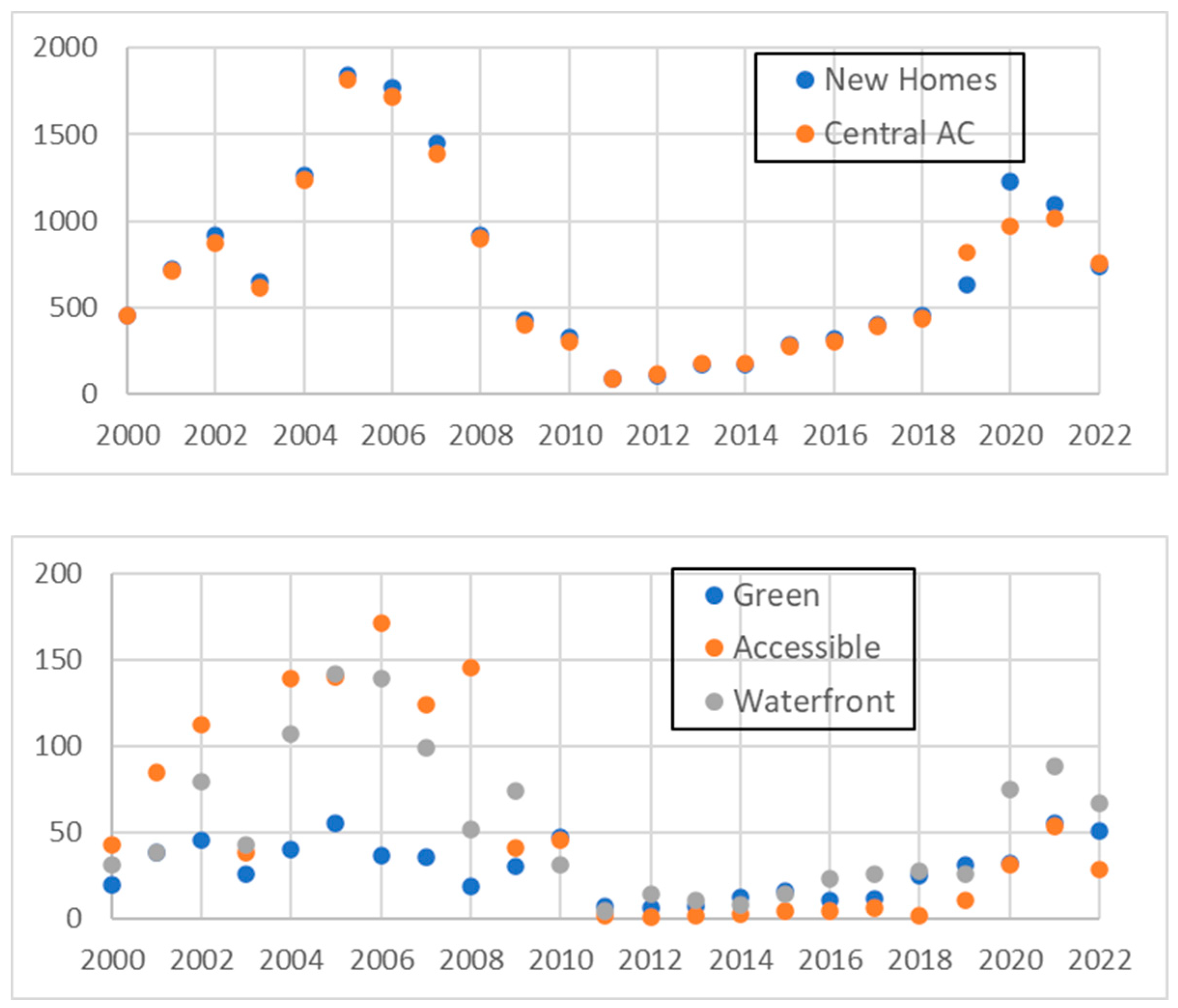
| Year | Av Price | New Homes | Accessible | Central AC | Green | Water- front |
|---|---|---|---|---|---|---|
| 2000 | 174,500 | 456 | 43 | 454 | 20 | 31 |
| 2001 | 187,800 | 718 | 85 | 716 | 38 | 38 |
| 2002 | 196,400 | 919 | 112 | 873 | 46 | 79 |
| 2003 | 203,400 | 649 | 38 | 615 | 26 | 43 |
| 2004 | 211,700 | 1267 | 139 | 1235 | 40 | 107 |
| 2005 | 222,000 | 1842 | 140 | 1815 | 55 | 142 |
| 2006 | 229,200 | 1775 | 171 | 1718 | 37 | 139 |
| 2007 | 233,800 | 1451 | 124 | 1386 | 36 | 99 |
| 2008 | 225,500 | 916 | 145 | 902 | 19 | 52 |
| 2009 | 212,000 | 427 | 41 | 401 | 30 | 74 |
| 2010 | 195,600 | 330 | 46 | 305 | 47 | 31 |
| 2011 | 180,500 | 89 | 2 | 88 | 7 | 5 |
| 2012 | 172,900 | 105 | 1 | 114 | 6 | 14 |
| 2013 | 183,400 | 168 | 2 | 174 | 7 | 11 |
| 2014 | 200,900 | 167 | 3 | 182 | 13 | 8 |
| 2015 | 216,600 | 283 | 5 | 277 | 16 | 14 |
| 2016 | 232,400 | 319 | 5 | 305 | 11 | 23 |
| 2017 | 249,100 | 404 | 6 | 394 | 12 | 26 |
| 2018 | 269,600 | 451 | 2 | 432 | 25 | 28 |
| 2019 | 286,400 | 629 | 11 | 823 | 31 | 26 |
| 2020 | 303,200 | 1225 | 31 | 968 | 32 | 75 |
| 2021 | 351,300 | 1091 | 54 | 1019 | 55 | 88 |
| 2022 | 430,000 | 740 | 29 | 760 | 51 | 67 |

| Factor | New Homes | Accessible | Central AC | Green | Water- Front | Price |
|---|---|---|---|---|---|---|
| raw data (Figure A1) | 0.729 | 0.368 | 0.757 | 0.544 | 0.632 | >0.990 |
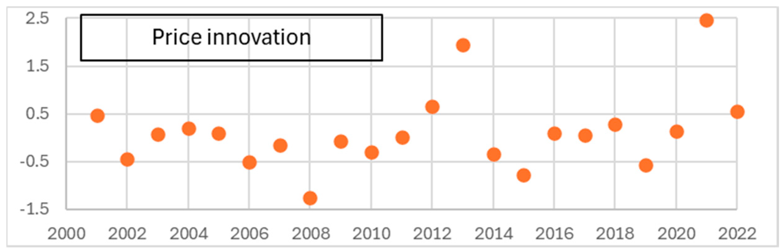
| arithmetic return | 0.074 | 0.012 | 0.069 | ** | ** | 0.943 |
| AR(2)-ARCH(1) innovation | na a | na | na | na | na | 0.020 |


| ATL | AUS | COL | JAX | NAS | OKC | POR | SEA |
|---|---|---|---|---|---|---|---|
| rtn a | rtn | rtn | rtn | rtn | rtn | rtn | rtn |
| rtn | rtn | rtn | rtn | rtn | rtn | rtn | rtn |
| rtn | rtn | fd b | rtn | rtn | rtn | rtn | rtn |
| rtn | rtn | rtn | rtn | rtn | rtn | rtn | fd |
| fd | fd | fd | fd | fd | fd | fd | fd |
| c | d |
Appendix C. GLM and GAM Residuals
| Year | ATL | AUS | COL | JAX | NAS | OKC | POR | SEA |
|---|---|---|---|---|---|---|---|---|
| 2001 | 0.068 | −0.229 | −0.082 | 0.050 | −0.101 | 0.001 | 0.218 | −0.025 |
| 2002 | −0.793 | −0.282 | −0.086 | 0.292 | −0.540 | −0.207 | −0.591 | −0.655 |
| 2003 | 0.246 | −0.608 | 0.394 | 0.244 | −0.332 | 0.253 | −0.100 | 0.773 |
| 2004 | −0.191 | 0.057 | −0.079 | 0.341 | −0.088 | −0.043 | 0.826 | 0.755 |
| 2005 | −0.411 | −0.034 | −0.004 | 0.005 | 0.828 | 0.322 | 1.577 | 0.700 |
| 2006 | −0.433 | −0.047 | −0.352 | −0.271 | 0.112 | 0.206 | −0.020 | −0.815 |
| 2007 | −0.053 | 0.251 | −0.089 | −0.198 | −0.481 | −0.577 | −0.196 | −0.780 |
| 2008 | −0.887 | −0.151 | 0.016 | −0.056 | −0.761 | −0.089 | 0.259 | −1.170 |
| 2009 | −0.416 | −0.354 | −0.188 | 0.289 | −0.243 | −0.485 | 0.294 | −0.067 |
| 2010 | −0.292 | −0.145 | −0.239 | −0.161 | 0.234 | −0.253 | −0.150 | −0.036 |
| 2011 | 0.319 | −0.039 | −0.341 | −0.171 | 0.319 | −0.024 | −0.699 | −0.275 |
| 2012 | 0.348 | 0.452 | 0.192 | −0.099 | 0.085 | 0.202 | −0.054 | 0.710 |
| 2013 | 1.857 | 0.326 | 0.333 | −0.018 | 0.137 | −0.407 | 0.180 | 0.150 |
| 2014 | −0.630 | 0.149 | 0.391 | −0.119 | 0.246 | 0.675 | −0.488 | −1.296 |
| 2015 | −0.948 | 0.072 | −0.092 | −0.300 | 0.616 | −0.312 | −0.718 | 0.347 |
| 2016 | 0.027 | −0.077 | −0.087 | 0.142 | −0.003 | 0.036 | 0.214 | −0.013 |
| 2017 | −0.151 | 0.228 | 0.219 | −0.158 | 0.406 | 0.070 | −0.116 | 0.921 |
| 2018 | −0.295 | −0.158 | −0.221 | 0.094 | −0.031 | 0.117 | −0.268 | −0.511 |
| 2019 | −0.387 | −0.026 | −0.156 | −0.006 | −0.498 | 0.273 | −0.561 | 0.225 |
| 2020 | 0.340 | −0.115 | −0.086 | −0.053 | −0.164 | −0.038 | −0.022 | 0.131 |
| 2021 | 2.152 | 0.657 | 0.259 | 0.189 | 0.148 | 0.144 | 0.717 | 1.027 |
| 2022 | 0.530 | 0.073 | 0.298 | −0.038 | 0.111 | 0.134 | −0.302 | −0.096 |
| Year | ATL | AUS | COL | JAX | NAS | OKC | POR | SEA |
|---|---|---|---|---|---|---|---|---|
| 2001 | 0.068 | −0.147 | 0.037 | −0.048 | −0.296 | 0.159 | −0.006 | 0.184 |
| 2002 | −0.793 | −0.530 | −0.232 | 0.119 | −0.463 | −0.369 | −0.052 | −0.686 |
| 2003 | 0.246 | −0.321 | 0.141 | 0.116 | −0.559 | −0.220 | −0.295 | 0.935 |
| 2004 | −0.191 | 0.195 | −0.126 | 0.601 | −0.304 | 0.000 | 1.535 | 0.945 |
| 2005 | −0.411 | 0.195 | −0.186 | −0.203 | 0.857 | 0.530 | 1.807 | 0.884 |
| 2006 | −0.433 | −0.019 | −0.591 | −0.293 | 0.045 | −0.481 | −0.784 | −0.704 |
| 2007 | −0.053 | 0.057 | −0.454 | −0.867 | −0.606 | −0.317 | −0.926 | −1.442 |
| 2008 | −0.887 | −0.190 | −0.397 | −0.025 | −0.967 | −0.607 | −0.414 | −1.151 |
| 2009 | −0.416 | −0.442 | −0.035 | 0.345 | −0.951 | −0.430 | −0.378 | −0.255 |
| 2010 | −0.292 | −0.404 | −0.195 | −0.034 | −0.164 | −0.536 | 0.167 | −0.122 |
| 2011 | 0.319 | −0.103 | −0.149 | 0.145 | 0.026 | −0.513 | −1.677 | −0.200 |
| 2012 | 0.348 | 0.443 | 0.392 | 0.015 | −0.324 | 0.654 | 0.363 | 0.707 |
| 2013 | 1.857 | 0.081 | 0.461 | 0.092 | 0.032 | −0.606 | 0.299 | 0.463 |
| 2014 | −0.630 | 0.172 | 0.516 | −0.078 | 0.688 | 0.971 | −0.090 | −1.100 |
| 2015 | −0.948 | −0.063 | 0.094 | −0.279 | 0.670 | −0.017 | 0.061 | 0.452 |
| 2016 | 0.027 | −0.220 | −0.370 | 0.329 | −0.141 | −0.481 | 0.483 | −0.051 |
| 2017 | −0.151 | −0.066 | 0.200 | −0.200 | 0.331 | −0.061 | −0.271 | 0.853 |
| 2018 | −0.295 | −0.450 | −0.053 | 0.009 | −0.348 | −0.383 | −0.289 | −0.469 |
| 2019 | −0.387 | 0.130 | −0.015 | −0.127 | −0.073 | 0.898 | −0.006 | 0.475 |
| 2020 | 0.340 | 0.036 | −0.113 | −0.051 | −0.308 | 0.032 | −0.385 | −0.006 |
| 2021 | 2.152 | 1.406 | 0.558 | 0.509 | 1.370 | 0.217 | 1.952 | 0.949 |
| 2022 | 0.530 | 0.240 | 0.517 | −0.044 | 1.483 | 1.560 | −1.092 | −0.660 |
| 1 | Data from https://www.zillow.com/homes/ were collected by specifying the city in the search field and then the entries for all filters as provided in Table A1 in Appendix A. |
| 2 | Home types considered are specified in the appropriate filter in Table A1. |
| 3 | Note that the data apply only to homes constructed within the city boundaries and not to homes within the associated Metropolitan Statistical Area. |
| 4 | Specifically, three of the factors are environmental and one (accessibility) is social, although all four are often influenced by local policies. |
| 5 | Restated in the context of the P-splined-based GAM and the GLM used here, extrapolation using polynomials is much less accurate than extrapolation using a linear least-squares fit. |
| 6 | In (5), we use a generic notation to denote the time series being tested. |
| 7 | denotes standard error. |
| 8 | We tested a variety of ARFIMA-GARCH models before settling on AR()-ARCH(1) with . We desired an ARFIMA-GARCH model that was as parsimonious as possible in the number of coefficients to be fit. |
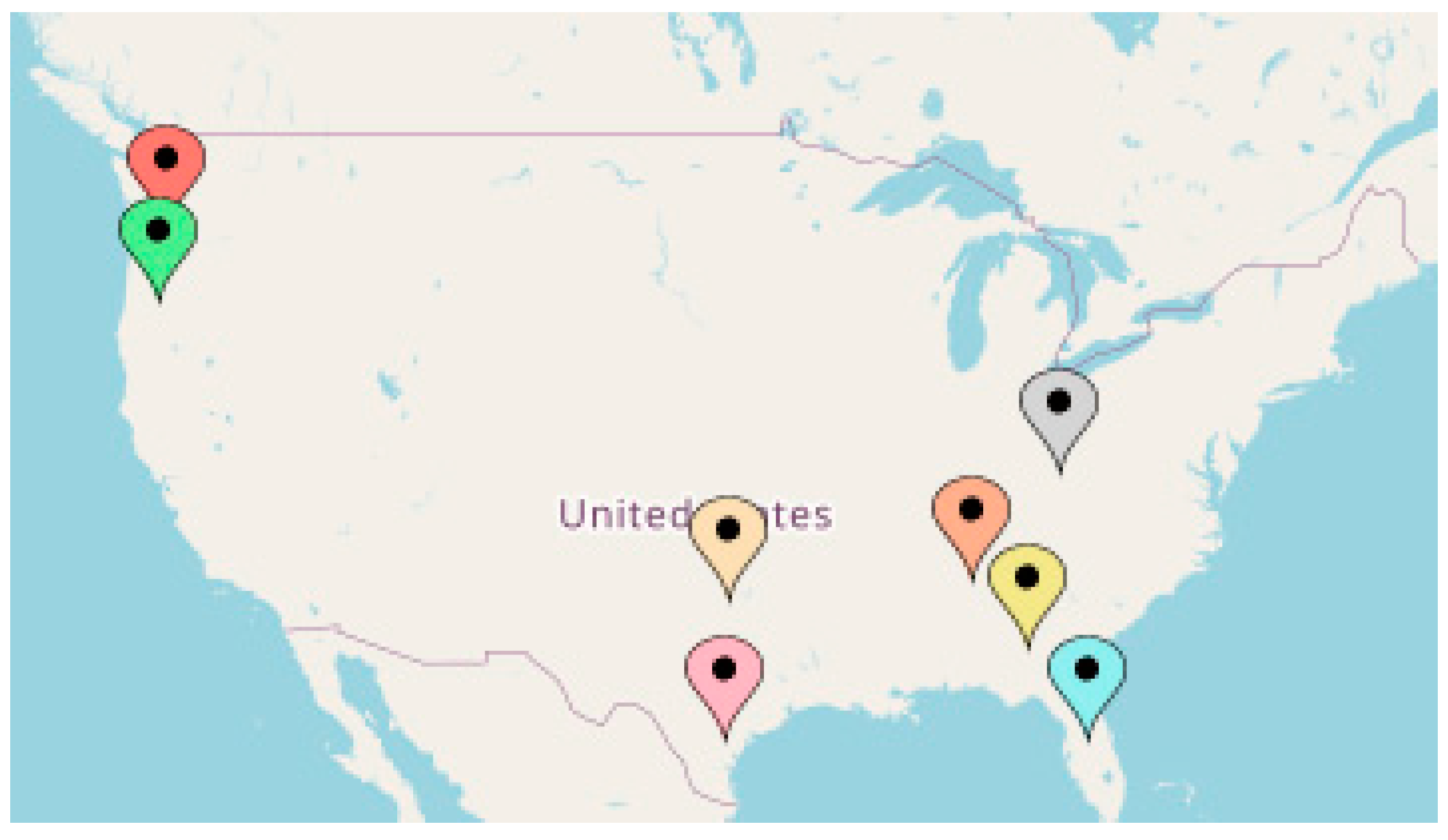
| 9 | We index the cities in alphabetical order. |
| 10 | The explained variance associated with each principal component is the ratio of its eigenvalue to the sum of all eigenvalues. |
| 11 | If two cities border a body of water in the United States, then the common city boundary often divides the body of water along a line medial to the city shorelines. Thus, two or more cities bordering a large and contained body of water can have large water-body percentages but relatively short shorelines. |
| 12 | Rebates and credits can be viewed at https://seattle.gov/city-light/residential-services/home-energy-solutions/heating-and-cooling-your-home#smartthermostatrebates (accessed on 5 August 2024). |
| 13 | Higher-order differences may be required if the time series is integrated of an order higher than one. |
References
- Bailey, Jason R., Davide Lauria, W. Brent Lindquist, Stefan Mittnik, and Svetlozar T. Rachev. 2022. Hedonic models of real estate prices: GAM models; environmental and sex-offender-proximity factors. Journal of Risk and Financial Management 15: 601. [Google Scholar] [CrossRef]
- Contat, Justin, Carrie Hopkins, Luis Mejia, and Matthew Suandi. 2023. When Climate Meets Real Estate: A Survey of the Literature; Working Paper 23-05; Washington, DC: Federal Housing Finance Agency.
- de Haan, Laurens, and Ana Ferreira. 2006. Extreme Value Theory: An Introduction. Berlin: Springer. [Google Scholar]
- Eilers, Paul H. C., and Brian D. Marx. 1996. Flexible smoothing with B-spines and penalties. Statistical Science 11: 89–121. [Google Scholar] [CrossRef]
- Hastie, T. 2023. Package ‘gam’. (V. 1.22-3). Available online: https://cran.r-project.org/web/packages/gam/gam.pdf (accessed on 3 July 2024).
- Lauper, Elisabeth, Susanne Bruppacher, and Ruth Kaufmann-Hayoz. 2013. Energy-relevant decisions of home buyers in new home construction. Umweltpsychologie 17: 109–23. [Google Scholar]
- Lavaine, Emmanuelle. 2019. Environmental risk and differentiated housing values: Evidence from the north of France. Journal of Housing Economics 44: 74–87. [Google Scholar] [CrossRef]
- Liao, Wen-Chi, and Xizhu Wang. 2012. Hedonic house prices and spatial quantile regression. Journal of Housing Economics 21: 16–27. [Google Scholar] [CrossRef]
- Mahanama, Thilini, Abootaleb Shirvani, and Svetlozar T. Rachev. 2021. A natural disasters index. Environmental Economics and Policy Studies 24: 263–84. [Google Scholar] [CrossRef]
- Ma, Junhai, Aili Hou, and Yi Tian. 2019. Research on the complexity of green innovative enterprise in dynamic game model and governmental policy making. Chaos, Solitons & Fractals: X 2: 1000008. [Google Scholar]
- Rachev, Svetlozar T., Stefan Mittnik, Frank J. Fabozzi, Sergio M. Focardi, and Teo Jašić. 2007. Financial Econometrics. New York: Wiley. [Google Scholar]
- US Census Gazetteer Files, United States Census Bureau. 2023. Available online: https://www.census.gov/geographies/reference-files/time-series/geo/gazetteer-files.2023.html (accessed on 14 January 2023).
- US Census, United States Census Bureau. 2010. Available online: https://www.census.gov/content/dam/Census/library/publications/2011/dec/c2010br-09.pdf (accessed on 17 September 2023).
- Zahid, R. M. Ammar, Adil Saleem, and Umer Sahil Maqsood. 2023. ESG performance, capital financing decisions, and audit quality: Empirical evidence from Chinese state-owned enterprises. Environmental Science and Pollution Research 30: 44086–99. [Google Scholar] [CrossRef] [PubMed]
- Zahid, R. M. Ammar, Muhammad Kaleem Khan, Umer Sahil Maqsood, and Marina Nazir. 2024. Environmental, social, and governance performance analysis of financially constrained firms: Does executives’ managerial ability make a difference? Managerial and Decision Economics 45: 2751–66. [Google Scholar] [CrossRef]
- Zeitz, Joachim, Emily Norman Zietz, and G. Stacy Sirmans. 2007. Determinants of House Prices: A Quantile Regression Approach. The Journal of Real Estate Finance and Economics 37: 317–33. [Google Scholar] [CrossRef]
- Zeitz, Joachim, G. Stacy Sirmans, and Greg T. Smersh. 2008. The Impact of Inflation on Home Prices and the Valuation of Housing Characteristics Across the Price Distribution. Journal of Housing Research 17: 119–38. [Google Scholar] [CrossRef]


| Factor | ATL | AUS | COL | JAX | NAS | OKC | POR | SEA |
|---|---|---|---|---|---|---|---|---|
| New Homes | 0.074 | ** | 0.017 | 0.034 | ** | 0.021 | ** | 0.014 |
| Central AC | 0.069 | 0.015 | 0.013 | 0.032 | 0.012 | 0.036 | ** | ** |
| Green | ** | ** | ** | ** | ** | ** | ** | ** |
| Accessible | 0.012 | ** | ** | 0.244 | ** | 0.076 | ** | ** |
| Waterfront | 0.015 | ** | ** | ** | ** | ** | ** | ** |
| Av Price Innovations | 0.020 | ** | 0.036 | 0.053 | 0.095 | 0.055 | 0.020 | 0.097 |
| Factor | ATL | AUS | COL | JAX | NAS | OKC | POR | SEA |
|---|---|---|---|---|---|---|---|---|
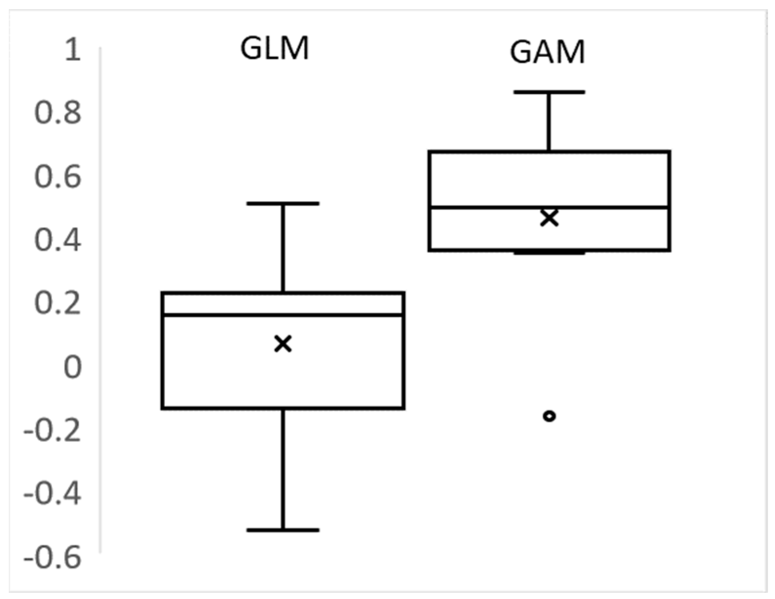
| GLM | ||||||||
| New Homes | 0.747 | 0.189 | 0.184 | 0.103 | 0.025 | 0.515 | 0.176 | 0.632 |
| Accessible | 0.467 | 0.994 | 0.169 | 0.315 | 0.585 | ** | 0.353 | 0.320 |
| Central AC | 0.594 | 0.234 | 0.169 | 0.117 | 0.024 | 0.700 | 0.550 | 0.879 |
| Green | 0.500 | 0.100 | 0.249 | 0.633 | 0.247 | 0.116 | 0.191 | 0.457 |
| Waterfront | 0.629 | 0.975 | 0.838 | 0.807 | 0.041 | 0.929 | 0.855 | 0.242 |
| Adj. | 0.167 | 0.061 | 0.144 | 0.159 | 0.218 | 0.504 | 0.525 | 0.226 |
| GAM | ||||||||
| New Homes | 0.747 | 0.151 | 0.100 | 0.017 | 0.091 | 0.152 | 0.017 | 0.555 |
| Accessible | 0.467 | 0.945 | 0.031 | 0.021 | 0.677 | ** | 0.720 | 0.169 |
| Central AC | 0.594 | 0.240 | 0.063 | 0.027 | 0.085 | 0.015 | 0.032 | 0.997 |
| Green | 0.500 | 0.019 | 0.356 | 0.188 | 0.102 | ** | 0.073 | 0.363 |
| Waterfront | 0.629 | 0.646 | 0.069 | 0.085 | ** | 0.984 | 0.123 | 0.462 |
| Adj. | 0.388 | 0.518 | 0.560 | 0.703 | 0.855 | 0.468 | 0.349 | |
| Number of significant factors | ||||||||
| Model | ATL | AUS | COL | JAX | NAS | OKC | POR | SEA |
| GLM | 0 | 1 | 0 | 0 | 3 | 1 | 0 | 0 |
| GAM | 0 | 1 | 4 | 4 | 3 | 3 | 3 | 0 |
| Number of cities for which a factor is significant | ||||||||
| Model | New Homes | Accessible | Central AC | Green | Water- front | |||
| GLM | 1 | 1 | 1 | 1 | 1 | |||
| GAM | 4 | 3 | 5 | 3 | 3 | |||
| ATL | AUS | COL | JAX | NAS | OKC | POR | SEA | |
|---|---|---|---|---|---|---|---|---|
| Water Area a | 0.7 | 2.0 | 2.6 | 14.5 | 4.2 | 2.3 | 7.9 | 40.9 |
| Seniors b | 3.8 | 4.6 | 7.2 | 7.9 | 8.2 | 13.4 | 9.0 | 4.1 |
| Model | PC 1 | PC 2 | PC 3 | PC 4 | PC 5 | PC 6 | PC 7 | PC 8 |
|---|---|---|---|---|---|---|---|---|
| GLM | 0.453 | 0.205 | 0.111 | 0.087 | 0.061 | 0.041 | 0.028 | 0.014 |
| GAM | 0.319 | 0.209 | 0.144 | 0.138 | 0.075 | 0.050 | 0.039 | 0.028 |
Disclaimer/Publisher’s Note: The statements, opinions and data contained in all publications are solely those of the individual author(s) and contributor(s) and not of MDPI and/or the editor(s). MDPI and/or the editor(s) disclaim responsibility for any injury to people or property resulting from any ideas, methods, instructions or products referred to in the content. |
© 2024 by the authors. Licensee MDPI, Basel, Switzerland. This article is an open access article distributed under the terms and conditions of the Creative Commons Attribution (CC BY) license (https://creativecommons.org/licenses/by/4.0/).
Share and Cite
Bailey, J.R.; Lindquist, W.B.; Rachev, S.T. Hedonic Models Incorporating Environmental, Social, and Governance Factors for Time Series of Average Annual Home Prices. J. Risk Financial Manag. 2024, 17, 375. https://doi.org/10.3390/jrfm17080375
Bailey JR, Lindquist WB, Rachev ST. Hedonic Models Incorporating Environmental, Social, and Governance Factors for Time Series of Average Annual Home Prices. Journal of Risk and Financial Management. 2024; 17(8):375. https://doi.org/10.3390/jrfm17080375
Chicago/Turabian StyleBailey, Jason R., W. Brent Lindquist, and Svetlozar T. Rachev. 2024. "Hedonic Models Incorporating Environmental, Social, and Governance Factors for Time Series of Average Annual Home Prices" Journal of Risk and Financial Management 17, no. 8: 375. https://doi.org/10.3390/jrfm17080375
APA StyleBailey, J. R., Lindquist, W. B., & Rachev, S. T. (2024). Hedonic Models Incorporating Environmental, Social, and Governance Factors for Time Series of Average Annual Home Prices. Journal of Risk and Financial Management, 17(8), 375. https://doi.org/10.3390/jrfm17080375