Abstract
Ocean wave energy is one of the cleanest renewable energy sources around the globe, but wave energy varies widely from place to place and from time to time. The long-term variability of wave power at 20 locations in the Indian shelf seas from 1979 to 2018 is described here using the European Centre for Medium-Range Weather Forecasts recently released ERA5 reanalysis hourly data. The variability is calculated on a yearly and monthly basis for the locations based on the coefficient of variation. The annual average wave power varied from 2.3 (at location 16 in the western Bay of Bengal) to 11 kW/m (at location 2 in the northeastern Arabian Sea). Along the western shelf seas, the maximum value of wave power is during the southwest monsoon period and along the east coast, it is during the tropical cyclone period. The standard deviation in wave power is more than the mean value at locations along the northern shelf seas of India, indicating a large variability in wave power in an annual cycle. The west coast locations are shown to have a slightly higher increasing trend with an average of 0.024 kW/m per year, while the increasing trend in wave power of east coast locations is with an average of 0.015 kW/m per year. The study also examines the variation in wave power from deep to shallow water at 2 locations using the wave characteristics obtained from the numerical model SWAN. The electric power output from a few wave energy converters are calculated for all the locations and found that the southernmost locations have a steady and higher percentage of power production.
1. Introduction
The depletion of conventional energy reserves, the rising cost of electricity generation and global warming have sparked interest in renewable ocean energy in many countries [1]. The oceans of the earth contain renewable energies in the form of tides, currents, waves, salinity gradient, and temperature gradient. The “Blue Economy” encourages better stewardship of our ocean or “blue” resources. Wave energy estimated worldwide by integrating the mean wave power on all coasts is 18,500 TW h/year or a mean power of ~2100 GW [2]. With the advancement in technology, ocean waves can become an economically viable renewable energy source [3]. There are a number of studies that describe the energy potential over global and regional scales based on wave data from buoys, numerical wave hindcasts, satellites, or a combination of these sources (see [4,5,6] for details). The annual average wave power is low at the equator and increases progressively toward the poles and it varies from 1 to 50 kW/m [1,4]. The early estimates of wave energy are based on wave buoy measurements. Now, most of the wave energy assessment studies are carried out either through the wave parameters obtained from a wave hindcast model or reanalysis data; ERA-40 or ERA-Interim [7] of the European Centre for Medium-Range Weather Forecasts (ECMWF).
As the global wave energy is fairly well understood, now the focus is shifting to the regional level for selecting suitable locations for the wave power plants. India, with a long coastline of 5423 km along the mainland [8], annually receives around 5.7 million waves [9]. Based on the ship reported deep-water wave data from 1968 to 1973, Rao and Sundar [10] estimated wave power that could be harvested around India. The Indian Institute of Technology (IIT) Madras in Chennai has conducted early studies on wave energy resources and a nearshore oscillating water column wave energy plant was installed on the southwest coast of India at Vizhinjam [11,12]. This wave energy plant is presently decommissioned. Based on the wave data measured using a waverider buoy for a one-year period, Sanil Kumar et al. [13] reported variations in wave power at four shallow water locations (water depth varying from 9 to 15 m) in the west and east coasts of India. Kumar and Anoop [9] reported the wave power at 19 deep-water locations in the Indian shelf seas based on ERA-Interim data. The distributions of wave-power potential along the Indian coastline have been reassessed from the last three-decade wave characteristics based on the numerical model [14]. Recently based on measured wave data at a location (~12 m water depth) in the central-eastern Arabian Sea (AS) from 2011 to 2017, the temporal distribution of wave power potential is reported by Amrutha et al. [15].
The Indian Ocean is in third place for its vastness among the world’s oceans. Indian Peninsula separates the North Indian Ocean (NIO) into two basins, AS and Bay of Bengal (BoB). Even though AS and BoB are at the same latitudinal belt, they have distinct wave nature due to the geographical features, variation in wind field and arrival of the swell field over the respective regions. Hence, the study covers locations in both AS and BoB and compares the wave power in these two basins. The wind pattern over NIO reverses its direction twice in a year. The annual mean wind field through the equatorial Indian Ocean is weak and westerly with a strong semi-annual westerly component during both inter-monsoons [16,17]. In general, the swell propagation in the Indian Ocean is always northeastward [9]. The variability in wave power arises due to variability in significant wave height and wave energy period, which arises due to variability in the wind. Nearer the coastline, the wave power decreases due to interaction with the seabed [18]. The wave energy resource at higher latitudes in both hemispheres tends to feature a strong seasonal variability. In contrast, the average level of wave energy in most equatorial regions (between 15° N and 15° S) remains steadier throughout the year. The main exceptions are the AS and BoB, which are seasonally affected by the southwest monsoon. Although several semi-equatorial regions are affected by tropical cyclones, typhoons, and hurricanes, the effects of these intermittent storms on time-averaged conditions do not appear significant [1].
A number of different wave energy converters (WECs) are developed worldwide based on different working principles [19]. WECs are classified based on how they interfere with waves, i.e., point absorbers (e.g., AquaBuOy), terminator (e.g., Salters duck) and attenuators (e.g., Wavestar) or based on the principle of operation, i.e., oscillating water columns (e.g., Backward Bent Duct Buoy), wave-activated bodies (e.g., Pelamis, WaveRoller, etc.), and overtopping devices (e.g., Wave Dragon) [19]. Some of the WECs are also depth-dependent. Around 600 MW wave power plants are installed worldwide and ~4 MW are fully operating [20], but most of them are test facilities working intermittently. The only exception is the Spanish facility in Mutriku (Spain), continuously supplying electricity to the grid now for more than five years [21]. The development of cost-effective models for grid integration of the electricity generated by an intermittent resource like waves is not an easy task [22]. Many theoretical frameworks have been developed and can be found in the literature [23]. However, again, as in Mutriku, where these developments have gone further as pre-operational models for managing electricity generated by waves [24].
Motivated by these aspects, the present study examines the wave power at 20 locations around the Indian mainland (Figure 1). Forty years of data is used in the study, which is higher than the minimum (~30 years) recommended by the World Meteorological Organization to make reliable estimations of climate variables in a region [25]. All the locations fall under deep to intermediate water depth. The details of the locations and mean wave characteristics are given in Table 1. The study also examines the capturing power of selected WECs at different locations.
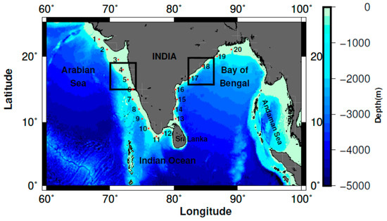
Figure 1.
Map showing the 20 locations selected in the Indian shelf seas for the study along with the bathymetry chart. The two boxes indicate the locations where the change in wave power from deep to shallow waters is examined.

Table 1.
The annual average value of significant wave height, mean wave period, wave power, and wave length at the locations studied along with their geographical position and the trend in annual mean wave power during the 40 years.
2. Data and Methodology
The significant wave height (Hs), mean wave period or energy wave period (Te), and peak period (Tp) data from the ERA5 global atmospheric reanalysis [26] produced by ECMWF are used in the study. The hourly data for the period from 1979 to 2018 at 20 locations are used in the study. Locations spaced ~1.5° latitude are selected. The ERA5 is the 5th generation of ECMWF reanalyzes of the global climate, having a spatial resolution of 31 km globally and the temporal resolution of one hour [26]. The wave data measured using directional wave rider buoy at 23 m water depth (15.465° N; 73.683° E) from 18 May 1996 to 17 May 1997 is used to compare the Hs, Te, and wave power from ERA5 data from the nearest grid point (15.5° N; 73.5° E). Measured data is a point measurement, whereas the ERA5 data is gridded data.
Wave parameters are converted to wave power per wave crest width (kW/m) by using the below expression (1) derived for deep waters. The wave power estimate based on this equation is ~5% less than that estimated based on equation suitable for shallow/intermediate waters [15]. Wave power referred here is the wave power density:
where ρ is seawater density (kg/m3) and g is gravitational acceleration (m/s2).
The temporal variability coefficients; coefficient of variation (COV), monthly variability index (MV), seasonal variability index (SV), as defined by Cornett [1], are used to study the variability/stability at different timescales. The yearly and monthly variation is studied based on COV for the locations. COV is the relative magnitude of the standard deviation (SD) divided by the mean value.
where PS1 is the highest seasonal average power, PS4 is the lowest seasonal average power, PM1 is the highest monthly average power and PM12 is the lowest monthly average power.
COV = SD/mean,
To delineate the tropical cyclone induced high wave power, the NIO cyclone track data obtained from Official US Navy Website Joint Typhoon Warning Centre (JTWC) is used. The trend in annual mean wave power is calculated based on the least-squares linear fit method. The slope of the linear best-fit curve to the annual average wave power for 40 years is estimated. A negative slope indicates the wave power decrease and positive slope an increase.
Third generation wave model SWAN is used to study the variations in wave power from deep water to shallow water at two domains, one each in AS and BoB (Figure 1). The bathymetry data used is ETOPO1. The grid used in the SWAN model is with a resolution of 1′. Wave frequencies are from 0.04 to 1 Hz over 25 bins on a logarithmic scale; 36 bins of 10° each are taken for direction. The JONSWAP formulation of the bottom friction coefficient value used in the study is 0.038 m2/s3. ERA5 bulk wave parameters are provided at the model boundaries. ERA5 hourly wind data is used to force the model. Wave power variation from deep water to shallow water during March, July, and November is examined.
The electric power output of different Wave Energy Converters (WEC) is estimated from the power matrix of each device for different years and the average value is presented. The performance of a particular WEC is evaluated using the capacity factor (Cf) and capture width (CW). CW is the portion of wave-front from which the WEC extracts the power.
where PE is electric power output from WEC, RP is the rated power of the system, PW is the available wave power.
ERA5 Hs data shows good comparison with the buoy data with a correlation coefficient of 0.98, root mean square error (RMSE) of 0.2 m and bias of 0.1 m. The annual mean Hs from ERA5 (1.3 m) compares well with the buoy (1.2 m) (Figure 2). The mean wave period shows a bias of 0.3 s and RMSE of 0.8 s. Here also, the annual mean value of the mean wave period compares well (7.3 and 7.1 s). Bias reported is the annual average of the deviation of ERA5 data with measured data. Annual mean wave power from ERA5 is 10.2 kW/m, whereas that from buoy data is 10.7 kW/m (Figure 2). Naseef and Kumar [27] reported that Hs values of ERA5 show a good agreement with the buoy data measured in the deep-waters (positive bias ~0.18 m) and coastal-waters (positive bias ~0.29 m) of the NIO. In the coastal waters, the annual average value of Hs is close to buoy data with a negative bias of 0.04 m in the eastern Arabian Sea and is within 3% of the measured Hs values in the western Bay of Bengal [27]. The annual mean Te of ERA5 is underestimated with a negative bias of 0.28 s in the western Bay of Bengal, whereas in the eastern Arabian Sea, overestimation is observed with a positive bias of 0.11 s [27].
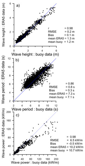
Figure 2.
Scatter plots of (a) significant wave height, (b) mean wave period, and (c) wave power from ERA5 and buoy.
3. Results and Discussion
3.1. Spatial Variation of Wave Power
The seasonal average wave power over the 40 years is calculated for the NIO and presented in Figure 3 for pre-monsoon (February–May), southwest (SW) monsoon (June–September), and post-monsoon (October–January) along with annual mean wave power. Over the NIO region, the maximum values of average wave power during annual, pre, southwest, and post-monsoon seasons are 17.73, 13.62, 39.87, and 12.63 kW/m, respectively. During the pre and post-monsoon period, the maximum values of wave power are found in the south-eastern part. In contrast, during the southwest monsoon, the maximum values are found at the northwestern, central AS and the Andaman Sea. Throughout the year, the wave power is less in the Indian shelf seas north of Sri Lanka due to the sheltering of the waves by Sri Lankan landmass. Earlier studies in coastal waters of India indicate an average wave power of 15.5 to 19.3 kW/m during the SW monsoon [13].
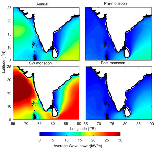
Figure 3.
Annual and seasonal mean wave power averaged over 40 years (1979 to 2018) for the study area in the North Indian Ocean during pre-monsoon (February–May), southwest monsoon (June–September), and post-monsoon (October–January).
3.2. Variations in Monthly Mean
The wave power at 20 locations is studied based on the variability at different time scale, such as monthly and annual from 1979 to 2018. The difference in the spatial distribution of monthly average wave power over the Indian ocean for different years is evident from Figure 4.
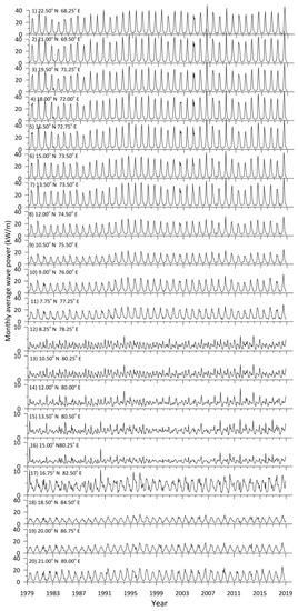
Figure 4.
Time series plots of monthly average wave power from 1979 to 2018 at the 20 locations in Indian shelf seas.
Due to the large seasonal variations and differences in wind patterns along the Indian shelf seas, large variations are observed in monthly mean wave power at each location and along the shelf seas. For locations 1–8, the range of monthly mean wave power for yearly data varies between 1 and 55.69 kW/m with the maximum wave power at locations 2 and 4. For locations 9 to 11, the wave power during the SW monsoon period is comparatively less than that at the northern locations (1–8) with the maximum at location 10 (31.5 kW/m) than the southernmost location 11 (29 kW/m). This difference in wave power in the northern, central, and southern locations in the eastern AS is due to the variations in the impact of the Findlater jet in the eastern AS [9]. In the eastern AS (locations 1–11), minimum wave power is observed during December-February and maximum in July (Figure 5). Whereas for locations in the western BoB (13 to 15), maximum wave power is observed in December and for locations 16 and 17, it is in May. The range of wave power at locations 18 to 20 is more due to the SW monsoon effect. For locations 13 to 17, wave power ranges from 0.5 to 10.6 kW/m and the minimum is observed during April at locations 13 and 14 and in February at locations 15, 16, and 17. For the locations 18–20, the minimum is observed in February and January and the maximum (16.24–26.32 kW/m) is observed in June and July. The wave power off the southeast coast of India is less than 5 kW/m due to the presence of Sri Lanka.
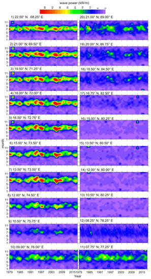
Figure 5.
Inter-annual variations in wave power from 1979 to 2018 at 20 locations depicted in month versus year plots.
The inter-annual variation of monthly mean wave power over the 40 years has a wide range (Figure 4). The percentage deviation of maximum wave power to mean in a particular month during the 40 years is always greater than that of the percentage deviation of minimum wave power to mean since most of the times all the locations had the occurrence of highest wave power either during monsoon or during the cyclones, which are extreme events. The lowest variation in the monthly mean wave power is for locations 11 and 12 (42–102%). The percentage variation during the SW monsoon period ranges from 42–136% and it arises due to the inter-annual variability of SW monsoon. The variability in the monsoon months is lower than that during the rest of the period. The percentage of variation is higher (54–250%) during the post-monsoon period due to the presence of cyclones.
Month-wise average wave power is calculated for the entire 40 years period. The monthly average wave power over 40 years for 20 locations (Figure 6) varied from 0.968 to 38.49 kW/m and the standard deviation varied from 0.2 to 7.43 kW/m. The monthly average wave power is maximum (11.9 to 38.5 kW/m) in July in the AS. For the AS locations, the maximum values of wave power are during the SW monsoon period. The difference in average wave power between July and June is comparatively higher for locations 1 to 6 than locations 7 to 10. For the southernmost location 11, the monthly average wave power varies between 5 and 20 kW/m with the maximum from June to September.
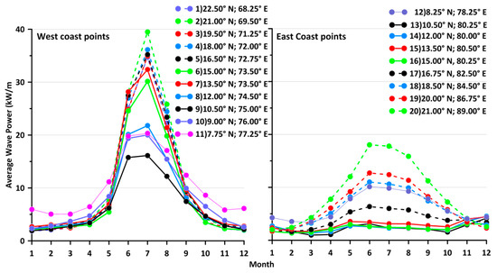
Figure 6.
Monthly average values of wave power at different locations. Left panel is for locations in the western shelf seas of India and the right panel is for the eastern shelf seas.
For BoB locations 13 to 16, monthly average wave power over 40 years is maximum (3.1 to 4.6 kW/m) in December and in the northwestern locations of BoB, the monthly maximum (6.2 to 17.6 kW/m) is in June. The monthly average wave power shows large variation over an annual cycle in most of the locations except at the southern locations (12 to 16). For the BoB locations between latitudes 16.75° N (location 17) and 21° N (location 20), the average wave power is maximum during the southwest monsoon period (5–20 kW/m) and maximum monthly average wave power is observed during June. For locations across 10.5° N to 15° N in the eastern shelf seas, the average wave power has range <5 kW/m with maximum values during December.
The power matrix of most of the WEC starts from 1m wave height and 4 s wave period and it contains around 2 kW/m wave power. Studies have shown that when the wave power is greater than 2 kW/m, it is feasible for the exploitation of wave energy from some WECs [28]. For some types of WECs like OWC, average values in the order of 20–30 kW/m of the wave energy flux are required to provide reasonable values of the capacity factor [29]. The total annual energy available and the exploitable energy for different locations are presented in Table 2. Exploitable energy considered in the present study is the sum of energy available in a year when the wave power is more than 2 kW/m and significant wave height less than 6.5 m. The southernmost locations show a higher percentage of occurrence of wave power greater than 2 kW/m (95% at location 12 and 99.3% at location 11). For west coast locations, the values are in between 71.5% (location 1) and 99.3% (location 11), whereas for east coast locations, the percentage of occurrence is ranging from 43 (location 13) to 95 (location 12). The annual exploitable energy at location 11 and 12 are 90.63 MWh/m and 53.83 MWh/m, respectively. The maximum exploitable energy of 93.70 MWh/m at the west coast is observed at location 2 and that of east coast location is 74.93 MWh/m at location 20. For the west coast, the total annual energy during the study period varied between 56.93 (location 9) and 96.45 (location 2) MWh/m. The total energy varied from 20 (location 16) to 77.15 (location 20) MWh/m for the east coast locations.
Table 2.
Percentage of time the wave power is available in different ranges for all locations studied. Total and exploitable storage of wave energy (kWh/m) are also presented. The values presented are the annual average for 40 years.
Monthly COV, which is normalized standard deviation by mean, for all the locations, is given in Figure 7. The COV had a range from 0.32 to 1.69. COV close to zero indicates low variability in wave power and greater than 1.2 is for locations having considerable variability. Minimum values of monthly COV for the locations varied between 0.32 (location 12) and 0.59 (location 13) is observed in January (location 20), February (location 19), April (3–8, 18), June (location 12), and July (location 1,2 and 11). Among 20 locations, the maximum values of COV varied between 0.49 and 1.69. For AS locations 5–9, the maximum COV values (0.77–1.01) are observed in May and for the remaining locations at AS, the maximum COV values are observed either February, November, or December. COV values of southernmost locations (location 11, 12) have a range of 0.32 to 0.52, which is not varying much as the rest of the locations. The high COV values (0.52–1.69) at BoB locations are mostly from October to December except at location 16, where the maximum COV value (1.69) observed in May.
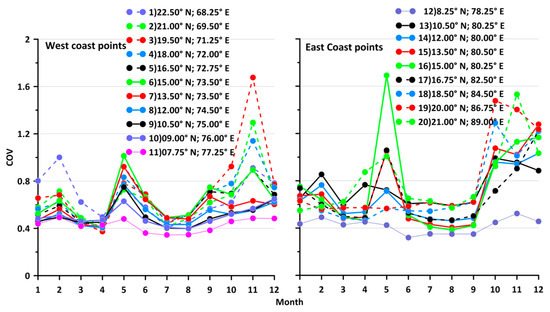
Figure 7.
Monthly coefficient of variation (COV) values at different locations. Left panel is for locations in the western shelf seas of India and the right panel is for the eastern shelf seas.
3.3. Variations in Annual Mean
Figure 8 gives the annual mean of wave energy flux during the 40 years. The annual mean wave power in the Indian shelf seas has a wide range (from 2.28 kW/m at location 16 to 11 kW/m at location 2). Among the locations studied, locations 1 to 5, 7, and 11 have relatively higher wave power (annual mean value >9 kW/m). For the BoB locations, the maximum annual mean wave power (8.8 kW/m) is in the northeastern area (location 20). The annual mean wave power in coastal water (~14 m water depth), which is 68 km from location 5 is 7.85 kW/m [15]. The annual mean power in the Indian shelf seas are comparable to the values reported in the tropical regions (E.g., North East Brazil (~2–14 kW/m), East and West peninsulas of Malaysia (~6.5 kW/m), Thailand (~10 kW/m), South China Sea (~5.32 kW/m) [20]. An earlier study shows that the annual average wave power in the coastal waters of India varied from 1.8 to 7.6 kW/m) [13]. For the BoB locations 13 to 17, low variability in average wave power is observed (small SD ~0.19–0.35 kW/m). For the rest of the BoB locations (18–20), the SD is in the range between 0.51 and 1.81 kW/m. On the other hand, for the AS locations, the SD varied from 0.57 (location 9) to 1.18 kW/m. During 1992–2000, 2007, 2018, there is an occurrence of high mean values of wave power compared to other years at the AS locations.
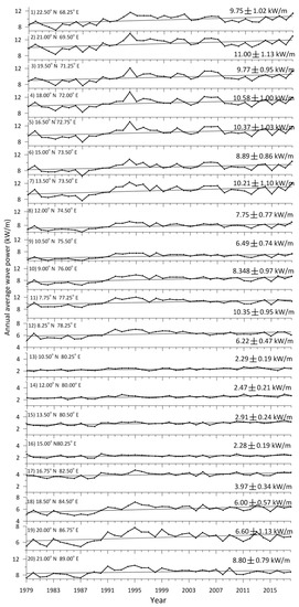
Figure 8.
Long-term change in annual mean wave power from 1979 to 2018 at the 20 locations. The annual average value and the standard deviations are also presented.
Sites with moderate and steady wave energy may well prove to be more attractive than sites where the resource is more energetic and unsteady. The variability coefficients COV, MV, and SV are calculated for the study locations on a yearly basis. The values are given in Figure 9. Values of MV and SV lower than 1 indicate moderate seasonal variability and large values indicate larger seasonal variability. For the southernmost points, the variation in the three coefficients is comparatively less, indicating steady wave power over an annual cycle. The maximum value (2.54) of COV is observed at station 16 during the year 1979. Lower COV (~0.7–0.8) is observed at locations 11 and 12. Overall the COV, MV, and SV of west coast locations are more than the southernmost points and east coast locations because of large SW monsoonal effect on the west coast, which causes large seasonal variations than on the east coast. As the overall variations in wave power over a year is less, the southernmost locations are ideal for selecting a wave power plant.
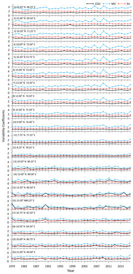
Figure 9.
Variability coefficients; coefficient of variation (COV), monthly variability index (MV), and seasonal variability index (SV) calculated based on yearly data for different years at 20 locations.
Information on the persistence of wave power availability at a location is required for investors for the planning of wave energy plants. Wave power availability above 10 kW/m and between 5 and 10 kW/m and less than 5 kW/m is presented in Table 2. The table shows that at the locations 1 to 7 in the northeastern AS, wave power from 5 to 10 kW/m is available in a year from 12% (locations 3 and 5) to 38% (location 11). Annually wave power more than 5 kW/m is available during 75% of the time at location 11 and 55% of the time at location 12. At locations 13 to 16, wave power more than 5 kW/m is available from 4% to 9% of the time only (Table 2).
The 25th percentile, 50th percentile, 75th percentile along with mean and SD of the wave power for the entire period is given in Figure 10. From the figure, it is clear that for locations 1 to 9, the 25th and 50th percentile values of wave power are similar, indicating that during 50% of the time in a year, identical wave conditions prevail along the region covering locations 1 to 9. The difference in the 50th and 75th percentile values of wave power for AS locations are in a larger range compared to BoB locations due to the SW monsoon. The influence of southwest monsoon on the waves is large in the AS and it will be predominantly from June to August. Hence, the 75th percentile values are high, i.e., during 25% of the time in a year, relatively high waves are in AS and these waves contain wave power more than 12 kW/m. SD is higher than the mean for locations 1 to 7. The mean values of wave power for locations 1 to 7 range from 7 to 11 kW/m and is close to the 75th percentile of the data set (10–13 kW/m), whereas the median or 50th percentile values of the data for these locations are very low (~4 kW/m). This again indicates that at locations 1 to 7, even though annual mean wave power is high (9–10 kW/m), during 50% of the time in a year, the wave power will be less than 4 kW/m. The SD is more than the mean and the maximum SD is observed at location 2. For locations 8 to 20, the SD is of the same range or less than the mean. This difference in SD is due to the southwest monsoon influence, which is evident from Figure 6. High wave power is observed during the SW monsoon period at locations 1 to 7 compared to 8 to 11. High wave power in November from 1981–1982 is due to cyclonic storms: Tropical storm one (1B) and cyclone 5 (5A). The maximum wave power is in June at all locations in the AS except at 9. At location 9, the maximum wave power is in May. At the southern locations in BoB (13 to 15), the maximum value is in December. At other locations in BoB, the maximum value is during the tropical cyclone (in May at locations 16, 17, 20 and in October at locations 18 and 19) (Table 3). Locations 11 and 12 have a consistently (i.e., small standard deviation) and high wave power on the annual cycle. At location 11, the mean and median value of annual wave power is close, indicating that around 50% of the time, wave power equal to annual mean value is available. During 25% of the time, wave power more than 13 kW/m is available at location 11.
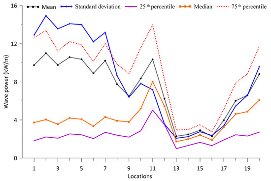
Figure 10.
Plots of mean, median, 25th percentile, 75th percentile, and standard deviation of wave power from 1979 to 2018 at 20 locations.
For AS locations (1 to 7), annually, the wave power varies from 0.2 to 393.1 kW/m. Considering the overall wave power data for a particular location, the maximum values of wave power over AS locations have a range of 57.8 kW/m (location 11) to 393.1 kW/m (location 2) (Figure 11). Most of the maximum wave power at these locations is observed during SW monsoon periods with the presence of cyclonic disturbance. The maximum wave power of 57.8 kW/m at the southernmost location (11) is observed on 22 February 2011, where no cyclones were observed. Whereas in the BoB locations, the range of maximum wave power is 65.7 kW/m at location 13 during cyclone BoB02 to 559.9 kW/m (location 20) during cyclonic storm Aila. Since extreme wave events determine WEC design conditions and its survivability, individual cyclone events are examined. The detailed representation of cyclonic disturbance during the period of maximum wave power at the location is given in Figure 12 and Table 3 represents the details of corresponding cyclones. There are 201 systems listed from 1979 to 2017, among them 144 formed in BoB and 57 in AS. But the Hs during most of the cyclones are less than 6.5 m. The power matrix of most of the WEC indicates that for Hs > 6.5 m, the power production is zero [30]. Only at locations 2, 3, 18, 19, and 20, maximum Hs is more than 6.5 m (Figure 11). For e.g., at location 20, the maximum Hs during the 40 years is 9.64 m, whereas Hs more than 6.5 m occurred only during 0.008% of the time in the 40 years. Hs more than 6.5 m occurred during cyclone Aila in May 2009, 1991 Bangladesh cyclone on 29 April 1991 and 1988 Bangladesh cyclone on 29 November 1988. Interestingly, there is no significant change in the annual average wave power at all the locations due to the cyclones. For e.g., at location 20, the annual average wave power considering all data is 8.80 kW/m, whereas the annual average excluding the three cyclones, which generated Hs more than 6.5 m is 8.78 kW/m. Similarly, at locations 2, 3, 18 and 19, the annual average wave power is 11.00, 9.77, 6.00, and 6.60 kW/m in both cases, i.e., excluding the cyclones and including the cyclones.
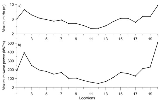
Figure 11.
(a) Maximum of the significant wave height at different locations and (b) the corresponding maximum wave power.
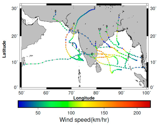
Figure 12.
Tropical cyclone tracks corresponding to the maximum wave power occurrence at different locations.
Table 3.
Details of the tropical cyclones represented in Figure 12. The list is as per the chronological order.
Table 3.
Details of the tropical cyclones represented in Figure 12. The list is as per the chronological order.
| No. | Maximum Wave Power (kW/m) (Location No.) | Date of Occurrence | Cyclone Name (IMD Classification) | Duration |
|---|---|---|---|---|
| 1 | 155.31 (16) 127.69 (17) | 12/5/1979 12/5/1979 | Cyclone One (1B) | 06/05/1979–12/5/1979 |
| 2 | 65.61 (13) | 3/12/1993 | BOB02 (ESCS) | 01/12/1993–04/12/1993 |
| 3 | 247.47 (03) 196.59 (04) 179.25 (05) 148.70 (06) 167.80 (07) | 18/06/1996 18/06/1996 17/06/1996 17/06/1996 17/06/1996 | ARB01(04A) (SCS) | 17/06/1996–20/06/1996 |
| 4 | 392.20 (02) | 08/6/1998 | ARB02(03A) (ESCS) | 04/06/1998–10/06/1998 |
| 5 | 103.78 (09) 77.59 (10) | 06/5/2004 | ARB01(04A) (SCS) | 05/05/2004–10/05/2004 |
| 6 | 189.58 (01) | 25/06/2007 | Yemyin (CS) | 21/06/2007–26/06/2007 |
| 7 | 504.07 (20) | 25/05/2009 | Aila (SCS) | 23/05/2009–26/05/2009 |
| 8 | 110.67 (14) | 30/12/2011 | Thane (VSCS) | 25/12/2011–31/12/2011 |
| 9 | 229.40 (19) | 12/10/2013 | Phailin (ESCS) | 06/10/2013–14/10/2013 |
| 10 | 211.41 (18) | 12/10/2014 | Hudhud (ESCS) | 07/10/2014–14/10/2014 |
| 11 | 168.98 (15) | 12/12/2016 | Varadah (VSCS) | 06/12/2016–18/12/2016 |
3.4. Long-Term Trend
In order to understand the trends and predict future wave power, a linear fit is made to the annual wave power from 1979 to 2018 for all the locations (Figure 8). The length of the data series used for trend analysis (40-year) is more than the period (30-year) recommended by the World Meteorological Organization [25]. The west coast locations are shown to have slightly higher increasing trend (varying from 0.016 to 0.037 kW/m per year with an average of 0.024 kW/m per year), whereas the increasing trend in wave power of east coast locations varied from 0.005 to 0.026 kW/m per year with an average of 0.015 kW/m per year. The increasing trend in wave power is in accordance with the changes in the wave height. At most of the locations, Hs showed an overall increasing trend during the 40 years. Global study indicates a sustained increase wave power in the Southern Ocean and a decrease in wave power in the North-Atlantic with the differences apparent mainly for the last decade [31]. From 2011 to 2017, year-to-year variability up to 13% is observed in annual mean wave power from the measured data for a location at 14 m water depth, which is 68 km away from location 5 [15]. The long-term variability is so small (0.96 kW/h in 40 years in the west coast locations and 0.6 kW/h in east coast locations), that it may be hindered by the expected error of the reanalysis.
3.5. Variation in Wave Power from Deep to Shallow Water
Wave power variation from deep water to shallow water during March, July, and November in 2015 at a specific latitude along longitudes with different depths in both AS and BoB is shown in Figure 13. In AS, 20 points are taken from 73.25–72.3° E with 0.05° interval and the depth varies from 6 to 55 m. The depth changes from 11.6 to 1136.46 m in BoB location from 83.35 to 83.95° E. The monthly mean wave power variation in March, July, November along the longitudes in AS is 2.58–3.29 kW/m, 14.09–34.49 kW/m, 2.22–3.26 kW/m. In BoB, the monthly mean wave power varies 6.71–4.43 kW/m 13.43–6.57 kW/m 7.71–6.10 kW/m during March, July, and November respectively along the longitudes. The reduction in wave power from deep to shallow water for AS location during March, July, November is 32%, 51%, and 56% respectively and for the BoB location, it is 36%, 50%, and 34%.
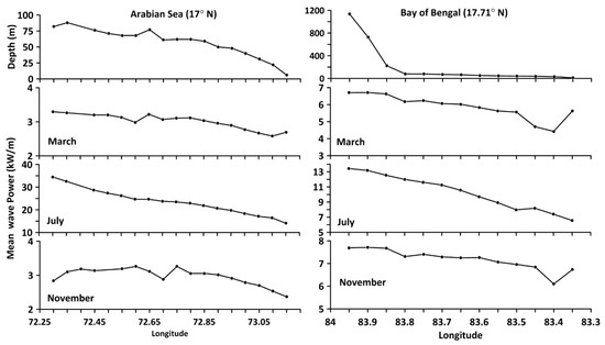
Figure 13.
Variation in wave power from deep water to shallow water. Left panel is for location in the Arabian Sea along 17° N and the right panel is for the location in Bay of Bengal along 17.71° N. Top panel is water depth and the other three are for March, July, and November 2015.
3.6. Performance of a Few Wave Energy Converters
Progress from full-scale testing to the commercialization of wave energy installations has been relatively slow, partly due to the financial risks associated with uncertainty in the wave energy resource assessment at a variety of timescales [32]. The performance evaluation of different devices for each location is carried out using the available power matrix of the technologies. The power matrix of different WECs available at different pieces of literature is used to estimate the electric power outputs at a particular location. Table 4 gives the different WEC used for this study and its operational depths. The power matrix is based on the wave period and Hs. Even though some of the power matrices are based on Te, Tm02, there is a majority using Tp. The comparison between power output based on Te and Tp is made for Oyster and Wavestar, where both the power matrix is available. The location 14 data are used for comparing the output power where the depth < 20 m. According to the power matrix using Te and Tp of the Oyster is having a rated power of 291 kW and 3332 kW, respectively. The rated power of Wavestar is 600 kW and 2709 kW for the power matrix based on Tm02 and Tp, respectively. In the case of Oyster, the percentage of zero power production is almost the same (~30%) from both matrices based on Te and Tp. For Wavestar, the percentage of zero production is negligible using Tm02 than using Tp (~30%) based power matrix. Hence, the wave power estimated from the power matrix of the WEC has to be used with caution since the power matrix is location-dependent and every device is specifically designed for a single location. The capture width of Oyster using Te is 11.71 m, and that uses Tp is 29.71 m. For Wavestar using Tm02, the CW is 54.41 m and that of Tp is 29 m. The capacity factor is also showing variation due to the rated power of the Tp matrix is more than that of Te. CETO, Oyster, and Wavestar Technology power matrix were used for the locations 14 and 12. For remaining locations that are at a water depth of >40 m, the rest of the technologies power matrix is used and given in Figure 14. Among the 20 locations, the southernmost locations 11 and 12 is having a maximum percentage of power production. Capture width is maximum for Wave Dragon with values from 74.75 m (location 11) to 183 m (location 16). The percentage time of zero power production for BBDB OWC is very short (0–17%) compared to the rest of the devices, but the capacity factor for BBDB OWC has a low range of up to 7% and the capture width ranges from 3.5 m to 5.5 m. In the absence of a realistic method to properly scale the power matrixes, the most efficient one for each location is considered.
Table 4.
Details of the wave energy convertors used in the study.
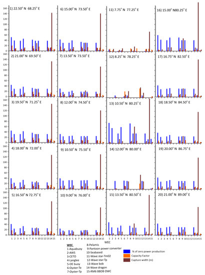
Figure 14.
Performance indices for different wave energy converters at the 20 locations based on yearly data for 2018.
One of the main challenges is that the WECs installed have to survive the harsh conditions in the site. The maximum Hs at the locations studied varied from 3.47 m (location 11) to 9.64 m (location 20). Among the west coast locations, the maximum Hs of 8.55 m is found at location 2. Sea states having a Hs of 4 m or more are less than 0.46% in an annual cycle, which corresponds to an incident average wave power of 80.8 to 102.1 kW/m. The wave conditions in the Indian shelf seas are not harsh, with Hs < 10 m and hence are favorable from the economic point of view. Only at locations 2, 3, 18 to 20, Hs exceeded 6.5 m and that too less than 0.007% of the time in the 40 years.
4. Conclusions
Wave power variability along the nearshore waters of India is studied from 1979–2018 by selecting 20 offshore locations covering the entire coast of the mainland. During the pre and post-monsoon period, the maximum values of wave power are found at the southernmost location. In contrast, in the southwest monsoon period, the maximum values are found at the northern and central AS. Twenty offshore locations covered in the study are at water depths 17 to 129 m situating 50 to 113 km from the coast. The difference between the 25th and 50th percentile values of wave power is similar for both AS and BoB locations. The difference in the 50th and 75th percentile values for AS locations are in a larger range compared to BoB locations. SD is higher than mean for locations AS lotions 1 to 7, and annually the wave power varies from 0.23 to 393.09 kW/m. Considering the overall wave power data for a particular location, the maximum values of wave power over AS locations have a range of 57.8 kW/m (location 11) to 393.1 kW/m (location 2). Most of the maximum wave power at these locations is observed during SW monsoon periods combined with the presence of weather disturbance, whereas in the BoB locations, the range of maximum wave power is 65.7 kW/m. The variability of wave power at different time scales, such as monthly and inter-annual periods, was obtained using the variability coefficients COV, MV, and SV. The minimum values of COV are observed at southernmost locations 11 and 12. Overall the COV, MV, and SV of west coast points are more than the southernmost points and east coast points because of larger SW monsoonal effect on the west coast than on the east coast.
The performance of different devices for each location was examined using the available technologies power matrix with the ratios, Cf and CW. The power matrix available for each device is based on Te, Tm02, and Tp. The comparison of the electric power output of Wavestar and Oyster are made using different power matrix. There is variation in the estimates of performance indices using different power matrix of the same WEC. Among the 20 stations, the southernmost locations (11 and 12) is having the maximum percentage of power production and moderate capacity factor. The reduction in wave power from offshore (55 m water depth) to coastal waters (6 m water depth) is 32% to 56% at different locations.
Author Contributions
Data downloading, analysis and original draft is made by M.M.A.; Data analysis, review and editing by V.S.K. All authors have read and agreed to the published version of the manuscript.
Funding
This research received no external funding.
Acknowledgments
CSIR-National Institute of Oceanography, India, provided facilities to carry out the research. ERA5 data used in this study is obtained from the ECMWF data server: http://data.ecmwf.int/data. We thank all the three reviewers for the constructive comments and suggestions which improved the content of the paper. The first author wishes to acknowledge CSIR for the award of Senior Research Fellowship. This work is done as part of the Doctoral thesis of the first author registered with Bharathidasan University, Tiruchirappalli and is an NIO contribution 6478.
Conflicts of Interest
The authors decleare no conflicts of interest.
Abbreviations
The following notations and abbreviations are used in this manuscript:
| ρ | seawater density |
| AS | Arabian Sea |
| BoB | Bay of Bengal |
| Cf | Capacity Factor |
| COV | coefficient of variation |
| CS | Cyclonic Storm |
| CW | Capture Width |
| ECMWF | European Centre for Medium-Range Weather Forecasts |
| ERA5 | fifth-generation ECMWF climate reanalysis data |
| ESCS | Extremely Severe Cyclonic Storm |
| g | gravitational acceleration |
| Hs | significant wave height |
| IMD | India Meteorological Department |
| JTWC | Joint Typhoon Warning Centre |
| MV | Monthly Variability index |
| NIO | North Indian Ocean |
| RMSE | Root Mean Square Error |
| SCS | Severe Cyclonic Storm |
| SD | Standard Deviation |
| SV | Seasonal Variability index |
| SWAN | Simulating WAves Nearshore |
| Te | mean wave period based on spectral moments m−1 and m0 or wave energy period |
| Tm02 | mean wave period based on spectral moments m0 and m2 |
| Tp | peak wave period |
| VSCS | Very Severe Cyclonic Storm |
| WEC | Wave energy converter |
References
- Cornett, A.M. A global wave energy resource assessment. In Proceedings of the ISOPE 18th International Conference on Offshore and Polar Engineering, Vancouver, BC, Canada, 6–11 July 2008. [Google Scholar]
- Gunn, K.; Stock-williams, C. Quantifying the global wave power resource. Renew. Energy 2012, 44, 296–304. [Google Scholar] [CrossRef]
- Clement, P.; McCullen, A.; Falcao, A.; Fiorentino, F.; Gardner Hammarlund, K. Wave energy Europe: Current status and perspectives. Renew. Sustain. Energy Rev. 2002, 6, 405–431. [Google Scholar] [CrossRef]
- Astariz, S.; Iglesias, G. The economics of wave energy: A review. Renew. Sustain. Energy Rev. 2015, 45, 397–408. [Google Scholar] [CrossRef]
- Barstow, S.; Mørk, G.; Mollison, D.; Cruz, J. The wave energy resource. In Ocean Wave Energy: Current Status and Future Perspectives; Cruz, J., Ed.; Springer: Berlin/Heidelberg, Germany, 2008; pp. 93–132. [Google Scholar]
- Aderinto, T.; Li, H. Ocean Wave Energy Converters: Status and Challenges. Energies 2018, 11, 1250. [Google Scholar] [CrossRef]
- Dee, D.P.; Uppala, S.M.; Simmons, A.J.; Berrisford, P.; Poli, P.; Kobayashi, S.; Andrae, U.; Balmaseda, M.A.; Balsamo, G.; Bauer, P.; et al. The ERA-Interim reanalysis: Configuration and performance of the data assimilation system. Q. J. R. Meteorol. Soc. 2011, 137, 553–597. [Google Scholar] [CrossRef]
- Kumar, V.S.; Pathak, K.C.; Pednekar, P.; Raju, N.S.N.; Gowthaman, R. Coastal processes along the Indian coastline. Curr. Sci. India 2006, 91, 530–536. [Google Scholar]
- Kumar, V.S.; Anoop, T.R. Wave energy resource assessment for the Indian shelf seas. Renew. Energy 2015, 76, 212–219. [Google Scholar] [CrossRef]
- Rao, T.V.S.N.; Sundar, V. Estimation of wave power potential along the Indian coastline. Energy 1982, 7, 839–845. [Google Scholar] [CrossRef]
- Raju, V.S.; Ravindran, M. Wave energy: Potential and programme in India. Renew. Energy 1997, 10, 339–345. [Google Scholar] [CrossRef]
- Mala, K.; Jayaraj, J.; Jayashankar, V.; Muruganandam, T.M.; Santhakumar, S.; Ravindran, M.; Takao, M.; Setoguchi, T.; Toyota, K.; Nagata, S. A twin unidirectional impulse turbine topology for OWC based wave energy plants—Experimental validation and scaling. Renew. Energy 2011, 36, 307–314. [Google Scholar] [CrossRef]
- Sanil Kumar, V.; Dubhashi, K.K.; Nair, T.M.B.; Singh, J. Wave power potential at few shallow water locations around Indian coast. Curr. Sci. 2013, 104, 1219–1224. [Google Scholar]
- Sannasiraj, S.A.; Sundar, V. Assessment of wave energy potential and its harvesting approach along the Indian coast. Renew. Energy 2016, 99, 398–409. [Google Scholar] [CrossRef]
- Amrutha, M.M.; Kumar, V.S.; Bhaskaran, H.; Naseef, M. Consistency of wave power at a location in the coastal waters of central eastern Arabian Sea. Ocean Dyn. 2019, 69, 543–560. [Google Scholar] [CrossRef]
- Schott, F.A.; McCreary, J.P. The monsoon circulation of the Indian Ocean. Prog. Oceanogr. 2001, 51, 1–123. [Google Scholar] [CrossRef]
- Schott, F.A.; Xie, S.P.; McCreary, J.P. Indian Ocean circulation and climate variability. Rev. Geophys. 2009, 47, RG1002. [Google Scholar] [CrossRef]
- Amrutha, M.M.; Sanil Kumar, V. Spatial and temporal variations of wave energy in the nearshore waters of the central west coast of India. Ann. Geophys. 2016, 34, 1197–1208. [Google Scholar] [CrossRef]
- Babarit, A. Wave Energy Conversion; Elsevier: Oxford, UK, 2017; p. 262. ISBN 9781785482649. [Google Scholar]
- Felix, A.V.; Hernández-Fontes, J.; Lithgow, D.; Mendoza, E.; Posada, G.; Ring, M.; Silva, R. Wave Energy in Tropical Regions: Deployment Challenges, Environmental and Social Perspectives. J. Mar. Sci. Eng. 2019, 7, 219. [Google Scholar] [CrossRef]
- Ibarra-Berastegi, G.; .Sáenz, J.; Ulazia, A.; Serras, P.; Esnaola, G.; García-Soto, C. Electricity production, capacity factor, and plant efficiency index at the Mutriku wave farm (2014–2016). Ocean Eng. 2018, 147, 20–29. [Google Scholar] [CrossRef]
- Reikard, G. Integrating wave energy into the power grid: Simulation and forecasting. Ocean Eng. 2013, 73, 168–178. [Google Scholar] [CrossRef]
- Reikard, G.; Robertson, B.; Bidlot, J.R. Wave energy worldwide: Simulating wave farms, forecasting, and calculating reserves. Int. J. Mar. Energy 2017, 17, 156–185. [Google Scholar] [CrossRef]
- Serras, P.; Ibarra-Berastegi, G.; Sáenz, J.; Ulazia, A. Combining random forests and physics-based models to forecast the electricity generated by ocean waves: A case study of the Mutriku wave farm. Ocean Eng. 2019, 189, 106314. [Google Scholar] [CrossRef]
- WMO. Calculation of monthly and annual 30-year standard normal: WCDP-No. 10. WMO-TD/No. 341; Technical Report; World Metheorological Organization, 1989; Available online: http://www.posmet.ufv.br/wp-content/uploads/2016/09/MET-481-WMO-341.pdf (accessed on 17 December 2019).
- Hersbach, H.; Dee, D. ERA5 reanalysis is in production. ECMWF Newsl. 2016, 147, 5–6. Available online: https://www.ecmwf.int/en/newsletter/147/news/era5-reanalysis-production (accessed on 17 December 2019).
- Naseef, T.M.; Kumar, V.S. Climatology and trends of the Indian Ocean surface waves based on 39-year long ERA5 reanalysis data. Int. J. Climatol. 2019. [Google Scholar] [CrossRef]
- Zheng, C.; Pan, J.; Li, J. Assessing the China Sea wind energy and wave energy resources from 1988 to 2009. Ocean Eng. 2013, 65, 39–48. [Google Scholar] [CrossRef]
- Rusu, E.; Onea, F. Estimation of the wave energy conversion efficiency in the Atlantic Ocean close to the European islands. Renew. Energy 2016, 85, 687–703. [Google Scholar] [CrossRef]
- Silva, D.; Rusu, E.; Soares, C.G. Evaluation of various technologies for wave energy conversion in the Portuguese nearshore. Energies 2013, 6, 1344–1364. [Google Scholar] [CrossRef]
- Reguero, B.G.; Losada, I.J.; Méndez, F.J. A global wave power resource and its seasonal, interannual and long-term variability. Appl. Energy 2015, 148, 366–380. [Google Scholar] [CrossRef]
- Neill, S.P.; Hashemi, M.R. Wave power variability over the northwest European shelf seas. Appl. Energy 2013, 106, 31–46. [Google Scholar] [CrossRef]
- Sinden, G. Variability of UK Marine Resources; The Carbon Trust: London, UK, 2005. [Google Scholar]
- Babarit, A.; Hals, J.; Muliawan, M.J.; Kurniawan, A.; Moan, T.; Krokstad, J. Numerical benchmarking study of a selection of wave energy converters. Renew. Energy 2012, 41, 44–63. [Google Scholar] [CrossRef]
- Sheng, W. Power performance of BBDB OWC wave energy converters. Renew. Energy 2019, 132, 709–722. [Google Scholar] [CrossRef]


© 2019 by the authors. Licensee MDPI, Basel, Switzerland. This article is an open access article distributed under the terms and conditions of the Creative Commons Attribution (CC BY) license (http://creativecommons.org/licenses/by/4.0/).