Abstract
A fault on the DC side of a flexible HVDC system, along with the rise in short-circuit current, develops rapidly. With the gradual expansion of flexible HVDC technology to large capacities and long-distance transmission and offshore transmission scenarios, the problem of short-circuit current calculation considering the characteristics of line distribution parameters needs urgent attention. Therefore, in order to solve the problem of the inaccurate calculation of the short-circuit current on the DC side, the lumped parameter model is used in a flexible DC system for long-distance transmission. This study analyzes the transmission line structure on the basis of the general model of the MMC short-circuit current calculation on the DC side and establishes a mathematical model of a long-distance transmission line considering the characteristics of distributed parameters. Two impedance equivalent models for different length lines are proposed to facilitate the analytical calculation of the short-circuit current. A short-circuit current calculation method for a flexible HVDC system with long-distance transmission lines is proposed. Additionally, the correctness of the proposed method is verified through the comparison of the simulation values and calculation values. The results show that the error of the lumped parameter calculation is about 10%, and the error of the distributed parameter calculation is less than 2%.
1. Introduction
The HVDC transmission mode based on a modular multilevel converter has many advantages, such as the flexible consumption of large-scale renewable energy, power supply to a passive network, independent control of the active/reactive power of the system, and the absence of the need to change the voltage polarity when the system power flow is reversed [1,2,3]. It has significant advantages in offshore wind farms, grid-connected new energy power generation, isolated island and weak grid power supply, asynchronous grid interconnection, and other projects and has broad development prospects [4,5].
In recent years, a number of long-distance flexible DC transmission projects have been completed and put into operation [6,7,8]. On 8 August 2023, China’s Hayu ±800 kV DC project officially began construction, with a total length of 2290 km of DC lines. In November, the Ganzhe DC project site conducted a selection survey on the use of fully flexible DC transmission technology, with a DC line length of 2368 km.
The continuous development and increasing application of MMC-HVDC have greatly improved the capacity, transmission distance of the system, and also significantly increased the probability of DC system short-circuit faults. In addition, the characteristics of MMCs, such as their small inertia and many energy storage components, lead to high rates of increase in short-circuit current and large overcurrent amplitudes, making it difficult for DC circuit breakers to be turned off. The increase in transmission distance makes an equivalent model of accurate and simple transmission lines particularly important for short-circuit current calculations. The above problems limit the further promotion and development of MMC-HVDC power grids [9,10,11,12]. Thus, the study of an effective equivalent model of long-distance transmission lines and the quantitative calculation of the MMC-HVDC short-circuit current on the DC side considering the line distribution parameters can not only provide a theoretical basis for the planning and design of multi-terminal flexible HVDC systems and the optimization of control and protection strategies, but it can also have important theoretical and engineering application value for seeking ways to reduce the fault current level.
There have been many studies on the calculation of the short-circuit current on the DC side of MMC-HVDC [13,14,15]. Based on a ±500 kV flexible DC transmission engineering model with symmetrical bipolar MMCs, authors [16] studied the circuit topology and its transient characteristics when different kind of faults occur. Then, they compared the effect of AC and DC circuit breakers to clear and recover various faults. Based on a single MMC short-circuit equivalent circuit, authors [17] studied short-circuit current calculation methods for a single converter valve considering a fault current limiter and arrester and analyzed the fault characteristics under different working conditions. Based on the RLC equivalent model, the pre-fault matrix of the multi-terminal converter station was derived from a single converter station [18], and the corrected fault matrix was established with several fault locations in order to solve the DC current of each branch. However, the method is not universal for the treatment of various faults in the MTDC power grid. In reference [19], considering that the MMC adopts constant DC voltage control, a short-circuit current calculation method with a differential equation was proposed. In reference [20], the dynamic method of a power supply and DC voltage controller based on a current differential equation was improved to provide the possibility of analyzing fault currents in the power grid under different operating conditions (such as fault resistance and limit inductance value). In reference [21], a fault current calculation method based on a coupled differential equation was proposed, and the short-circuit current of the MMC with and without locking was calculated using a complex differential equation. In reference [22], the authors provide a calculation method for the short-circuit current before MMC blocking by establishing a linearized model of a modular multilevel converter, but different model forms need to be built for different faults.
HVDC transmission systems usually use overhead lines for transmission. Due to the frequency change characteristics of line parameters, when the transient electric gas is transmitted along the transmission line at different frequencies, its propagation speed and attenuation coefficient are significantly different [23,24]. The authors of reference [25] greatly increased the difficulty of the analytical calculation for flexible transmission system DC short-circuit currents. In reference [26], a transmission line model in the phase domain was established based on the relationship between phase current and voltage at the transmitting and receiving ends of single-phase lines, and the relationship established by the ABCD matrix was extended to polyphase lines. In reference [27], the distribution parameter characteristics and frequency variation characteristics of transmission lines were considered, and the AC system with long-distance transmission cables was made equivalent by using the vector matching method. However, the distributed parameter line models provided by these studies mainly focus on AC transmission systems.
For HVDC systems, reference [28] considers the influence of mutual inductance, uses the measured inverse sequence current and fault inverse sequence current to calculate the phase and amplitude of the voltage, and performs fault location by solving the phase mutation point of the fault location function. The authors of reference [29] sharply consider the effects of distribution parameters and frequency-related line parameters, propose an improved frequency-dependent line model based on convolution, and design a convolution-based time-domain fault location algorithm. However, the above literature mainly considers the fault location problem in the equivalent of the distributed parameter line model, and it does not study the transmission line model suitable for the calculation of DC short-circuit current.
Considering the distributed parameter model, a method for calculating the short-circuit current of a flexible HVDC system with distributed parameters is proposed. Firstly, the distributed parameter circuit model of a line unit length element is established, the transmission line equation is derived, and the steady state expression of voltage and current is obtained using a wave equation, to calculate the line impedance. Different line impedance equivalent models are studied, and different model equivalents for different fault distances are proposed to reduce the calculation error. The correctness of the calculation method is verified by comparing the simulation value with the calculated value.
2. Transmission Line Equation
The unit length parameters of the transmission line include the resistance, reactance, conductance, and susceptance of the unit length line. In the calculation, the split wire may be replaced with an equivalent wire. The reactance value and susceptance value can be determined according to the expression of the single-core wire. The resistance and conductance values are independent of the shape of the transmission line, where the resistance value is determined by the number of wires per pole, while the conductance value depends on the corona active power loss and leakage on the insulation, and due to their small values, they are usually ignored in practical calculations.
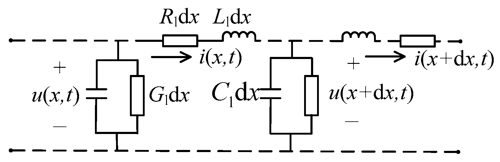
The theory of a uniform transmission line assumes that the parameters of any section of the power are evenly distributed along the transmission direction. It has nothing to do with the line structure and the transverse and longitudinal distribution of the electromagnetic field, and it only considers the changes in current and voltage along the line. Taking unipolar lines as an example, the distributed parameter equivalent model of long-distance transmission lines is studied. A power line with a length of x is divided into many infinitesimal length elements dx; then, each length element of dx has resistance Rldx and inductance Lldx and has capacitance Cldx and conductance Gldx between the line and the ground. The structure is shown in Figure 1.

Figure 1.
Distributed parameter line unit length element circuit model.
Let the unit length resistance, inductance, conductance, and capacitance be constant, and the transmission line equation applicable to any excitation source can be listed as shown in Equation (1).
In a distributed parameter line, the voltage to ground and the line current at any location are functions of time and distance, in line with the principle of electromagnetic wave propagation along the route; then, the wave process of a unipolar line can be expressed through partial differential equations, as shown in Equations (2) and (3):
The wave equation can be obtained from Equations (2) and (3):
where v is the propagation speed along the wave, and .
The D’Alembert solution of Equations (4) and (5) is as follows:
where u+ and i+ are the voltage and current with a velocity v propagating in the positive direction of x; u− and i− are voltages and currents with a velocity of v propagating in the opposite direction of x. The individual u+, u−, i+, and i− are all solutions to the wave equation, and they propagate independently, complementally interfering.
The characteristic equation in the time domain can be obtained from Equations (6) and (7):
When the system is in a stable state, the voltage and current can be expressed as follows:
where is the propagation coefficient, is the characteristic impedance, is the line impedance per unit length, and is the admittance per unit length.
A simple two-terminal MMC-HVDC is shown in Figure 2. The current is transmitted from MMC 1 to MMC 2, and the total length of the transmission line is L. When the voltage and current at one end are known, the relationship between the voltage and current at both ends of the line can be expressed, as shown in Formulas (11) and (12).
where subscript A represents the amount of electricity propagating in the positive direction, and subscript B represents the amount in the opposite direction.

Figure 2.
Two-terminal MMC-HVDC transmission system.
The above formula is the distribution parameter expression of the line, but it does not consider the frequency change. Since the resistance per unit length of the transmission line is positively correlated with the frequency, and the inductance is negatively correlated with the frequency, that is, different frequencies make the impedance of the line different, showing different transmission characteristics, it is necessary to correct the line impedance.
where is the resistance per unit length of the line when the frequency is f0.
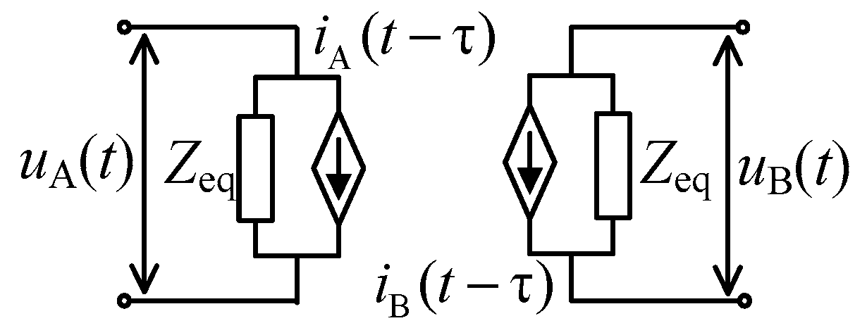
By converting the voltage and current relationship between the two ends of the line into the time domain, the equivalent circuit of the line distribution parameter model can be obtained, as shown in Figure 3. The first and last ends of the line are connected in parallel by an initial current source to the ground branch and the equivalent impedance, and the first and last ends are physically independent of each other and are interconnected through the electromagnetic relationship of the current source.
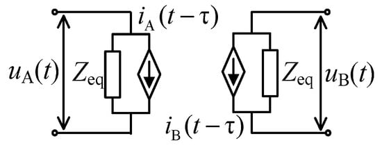
Figure 3.
Equivalent circuit of distributed parameter model.
The above model does not consider the line frequency characteristics, and a lossless line model is established according to the traveling wave method, where the equivalent impedance and current source can be expressed as follows:
In the formula, L0 and C0 are the fundamental frequency inductance and capacitance of the per length element line, respectively.
3. Line Equivalent Model with Distributed Parameters
Based on the steady-state transmission model, the distributed parameter model of long-distance transmission lines can be further derived. According to Equations (2) and (3), the transmission line model can be equivalent to the standard two-port model according to the sending and receiving ends, as shown in Figure 4, and the voltage and current of the two-port network can be expressed as Formula (20):
where A, B, C, and D are the elements of the two-port transmission matrix, , , .
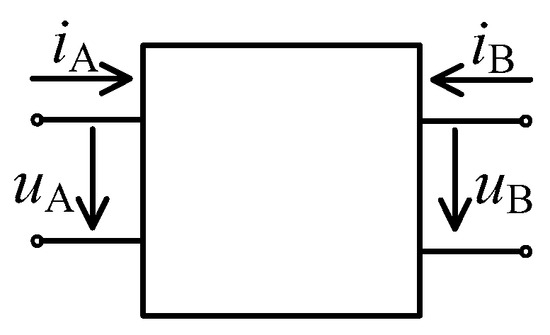
Figure 4.
Two-port network model for transmission lines.
According to the two-port theory of the circuit, the two-port network can be equivalent to a π-type circuit, and the equivalent impedance and admittance in the circuit can be expressed as follows:
3.1. Equivalent Model of Transmission Line Correction Coefficient
To facilitate the analytical calculation of the short-circuit current, the equivalent impedance of the line is simplified, and the wave impedance ZC in Equations (21) and (22) is expressed by the impedance parameters Z0 and Y0 per unit length of the line, as shown in Equations (23) and (24).
where ks and ky are the correction coefficients for calculating the characteristics of the line distribution parameters, and L is the line length.
The correction coefficients of resistance, reactance, and susceptance in the π-type equivalent circuit can be obtained by decomposing the Taylor series of Equations (23) and (24), ignoring the quadratic and smaller series terms and sorting out the real and imaginary parts of the equations.
where
The impedance of the π equivalent circuit can be derived from the above correction coefficients:
Taking a 500 kV line as an example, where resistance rl = 0.02 Ω/km, reactance xl = 0.28 Ω/km, and capacitance cl = 0.0129, the correction coefficients of the resistance, reactance, and capacitance of the π-type equivalent circuit of different line lengths can be calculated, as shown in Table 1.

Table 1.
Equivalent impedance correction coefficient of different length lines.
As can be seen from the above table, when the line length is less than 300 km, the correction factor of the impedance is about equal to 1, and the error is less than 2%, which can be calculated with the lumped parameter model. When the line length is 300–500 km, the modified coefficient method can better characterize the line impedance parameters. When the length is greater than 500 km, the error of the impedance correction coefficient is greater than 5%, and a more accurate model is needed to calculate the line parameters.
3.2. Gorev Equivalent Model of Transmission Line
The essence of the Gorev method is to convert hyperbolic functions containing complex variables into trigonometric functions, which can obtain more accurate line equivalent parameters than the lumped parameter model and linear modified impedance parameter coefficient model. The Gorev method first assumes that corona power loss in the line is ignored, gl = 0, so the propagation coefficient and wave impedance ZC can be expressed as follows:
By comparison, it can be seen that the second factor of Equations (31) and (32) is the same, and the first factor corresponds to the phase coefficient and wave impedance of the line, respectively. The second factor is decomposed by power series, and the series term of more than two times is ignored.
According to Equations (25)–(27), ; therefore,
By substituting Equation (35) into Equations (24) and (25), a simplified expression of the impedance can be obtained:
When the line is long, the transmission line can be made equivalent according to the line length by using the modified coefficient model and the Gorev model. When the line is short, the equivalent impedance and admittance of the line can be approximated as , , . Therefore, the approximate values of the equivalent impedance and admittance can be obtained:
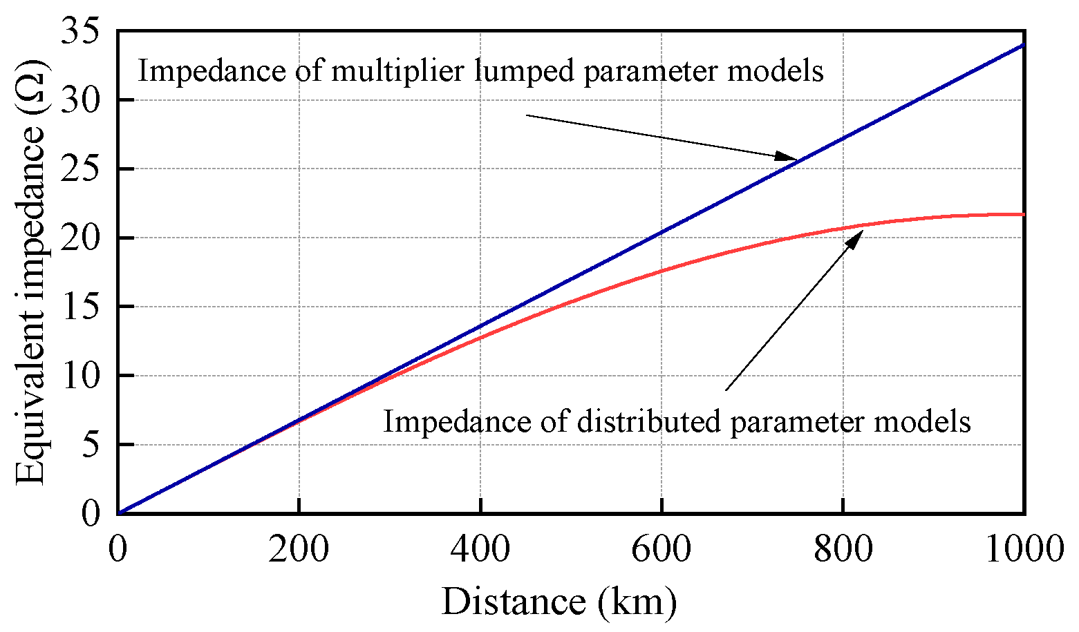
From the above analysis, it can be seen that Equations (38) and (39) are multiplier lumped parameter models, which can be understood as a simplified form of the line distribution parameter model. By comparing the above approximate impedance methods, it can be seen that the lumped parameter model is suitable for the power grid with short lines. Taking the two-terminal network as an example in Figure 2, the equivalent circuit reactance error of the lumped and the distributed parameter models is compared for the circuit, and the results are shown in Figure 5.
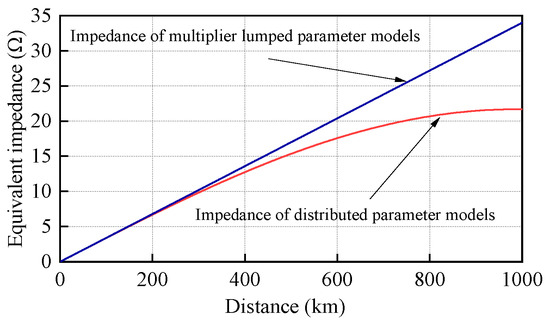
Figure 5.
Comparison of circuit equivalent reactance between lumped parameter model and distributed parameter model.
As shown in Figure 5, when the line length is less than 300 km, the equivalent reactance calculated by the lumped and the distributed parameter models is basically equal; however, when the line length exceeds 350 km, the deviation in the equivalent reactance between the lumped and the distributed parameter models gradually increases with an increase in the line and reaches about twice the error at 1000 km, which is unacceptable. The equivalent reactance of the lumped parameter model is proportional to the line length, while the equivalent reactance of the distributed parameter model is nonlinear with the line length.
4. Short-Circuit Current Calculation Method for Flexible DC Transmission System with Distributed Parameters
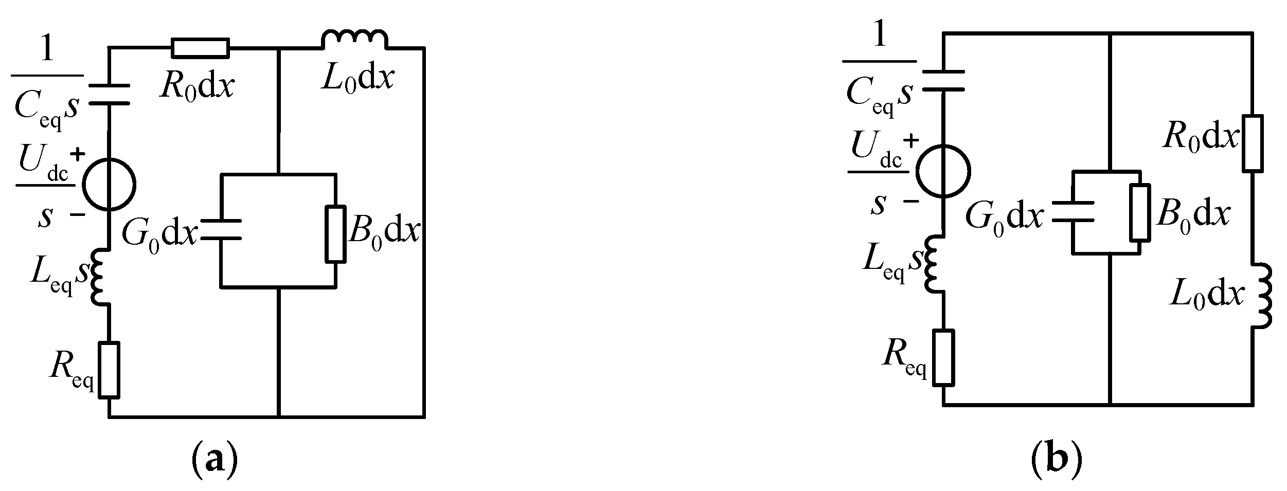
In order to provide a more direct theoretical basis for practical engineering planning and equipment selection, it is necessary to put forward a simple and universal analytical calculation method for short-circuit currents, so the influence of interference is ignored. According to the distance between the fault point and the discharge converter station, the impedance value of the DC line is calculated using different line equivalence methods. When the line length is less than 300 km, the lumped parameter method can be used to calculate the impedance value directly. When the line length is 300–500 km, the circuit impedance is calculated with the modified coefficient method to solve the short-circuit current. When the line length is greater than 500 km, the Gorev method line equivalent model is used for calculation. The equivalent circuit of MMC discharge with different line equivalent models is shown in Figure 6.

Figure 6.
MMC discharge equivalent circuit with long-distance transmission line. (a) T-type equivalent model. (b) π-type equivalent model.
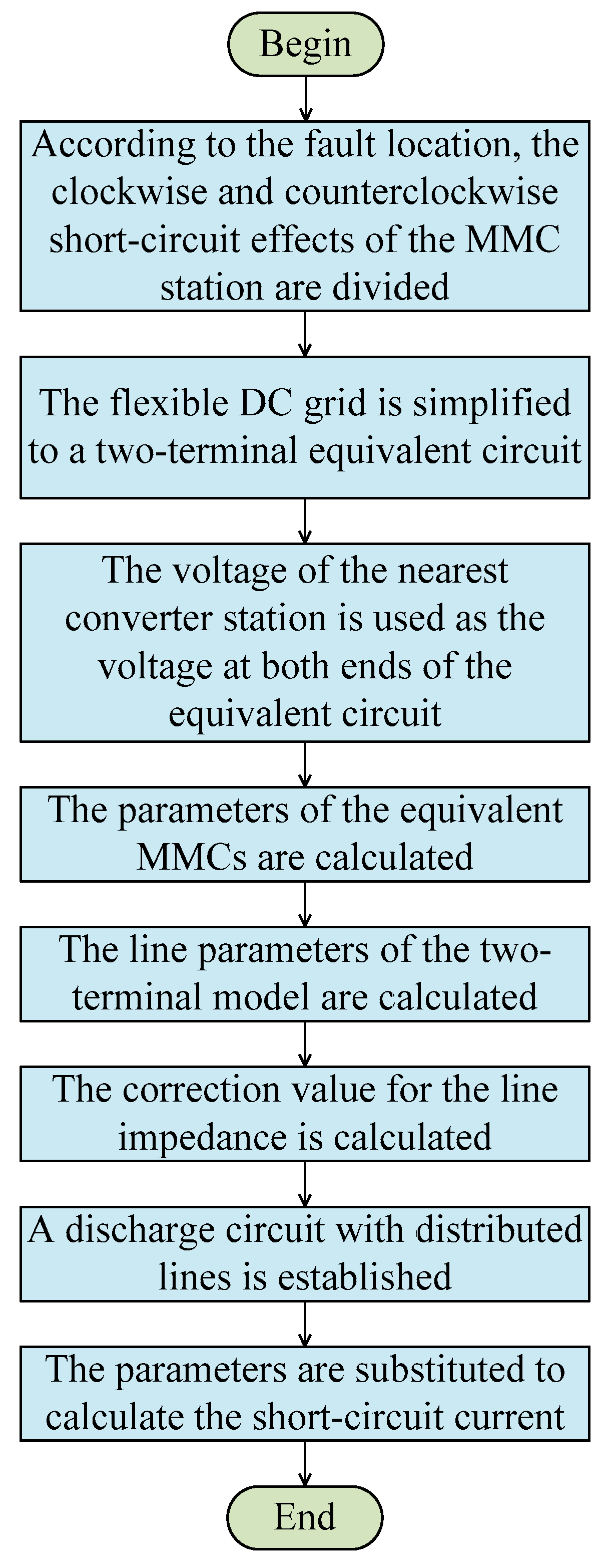
Based on the expression of the MMC DC short-circuit current [11], the equivalent value of the DC line impedance obtained in the previous study is used to replace the line impedances Ldc and Rdc represented by the lumped parameter model in the analytical expression when the short-circuit current is actually solved. The analytical expression of the short-circuit current on the DC side of the flexible HVDC system considering long-distance transmission lines can be obtained, as shown in (40), and the calculation process is shown in Figure 7.
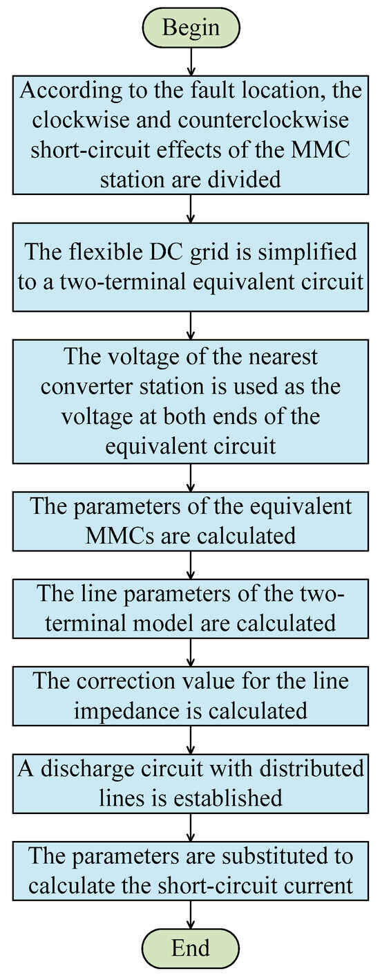
Figure 7.
Short-circuit current calculation flow chart.
5. Simulation Verification
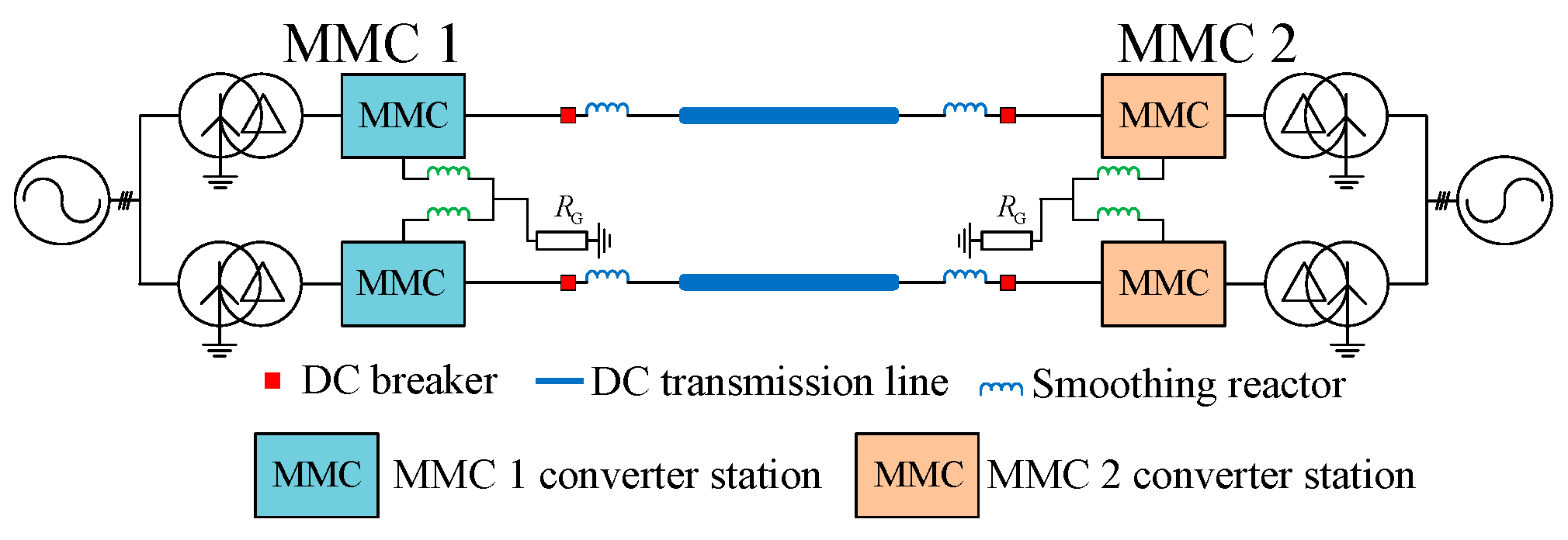
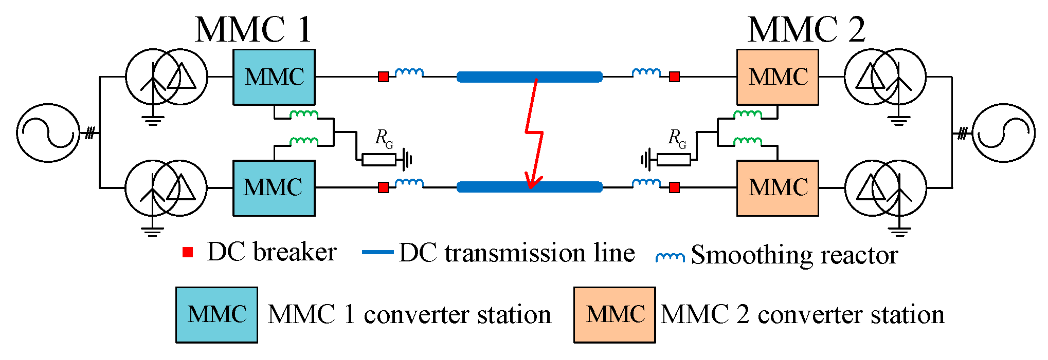
A two-terminal flexible DC transmission system model is built based on the PSCAD/EMTDC, as shown in Figure 8. The line length L is 2000 km, and the simulation step is 50 μs. The overhead line frequency-dependent phase domain model is adopted for the DC transmission line. Table 2 and Table 3 list the parameters of the MMC station and transmission line. A gold pole-to-pole short-circuit fault occurred on the line between MMC 1 and MMC 2.

Figure 8.
Two-terminal MMC-HVDC system with long-distance transmission lines.
Table 2.
The parameters of the MMC in the two-terminal system.
Table 3.
The major parameters of the line.
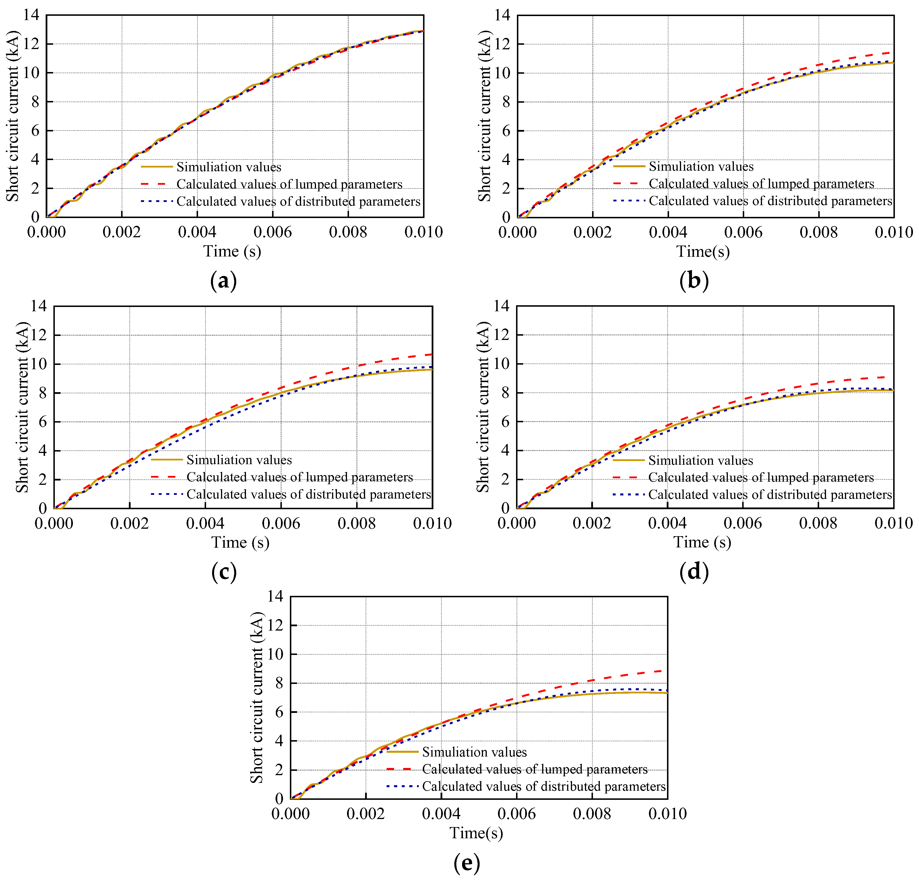
When the distance between MMC 1 and the fault is L = 0 and there is no transmission line, the short-circuit current can be calculated directly using an analytical expression. When the distance between the fault point and the converter station is not 0, the short-circuit current should be calculated according to the flow diagram in Figure 7, considering the distribution parameter characteristics and frequency variation characteristics of the line. Figure 9a–e show the comparison of simulation values with those calculated with the lumped parameter model and the distributed parameter model under the working conditions of 0 km, 600 km, 1000 km, 1600 km, and 2000 km between the fault point and MMC 1, respectively. Table 4 shows the errors between the simulated values for different fault distances and the calculated values for the line lumped and distributed parameter models, which is the average of the error at each time within 10 ms.
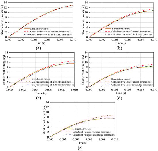
Figure 9.
A simulation and calculation comparison of different fault locations. (a) The fault is 0 km away from MMC 1; (b) the fault is 600 km away from MMC 1; (c) the fault is 1000 km away from MMC 1; (d) the fault is 1600 km away from MMC 1; (e) the fault is 2000 km away from MMC 1.
Table 4.
Error comparison of calculated values at different fault locations.
From the above comparison results, when short-circuit faults occur at different locations, the distributed parameter model considering frequency variation characteristics can calculate the short-circuit current, and the error between the calculated current and the simulated current is small. With an increase in the distance between the MMC and the fault, the increase in short-circuit current decreases gradually. When the fault occurs at the outlet of the converter station, the analytical calculation values of the short-circuit current determined using the lumped parameter model and distributed parameter model can be accurately fitted to the simulation values. But when the fault is far away from the converter station, the analytical calculation of the short-circuit current using the lumped parameter model has a greater average error within 10 ms. When the line length is set to 0 km by the distributed parameter model, there is a small ripple in the simulation values of the short-circuit current, which makes the calculation error of the distributed parameter seem larger than that of the lumped parameter. But it can be ignored.
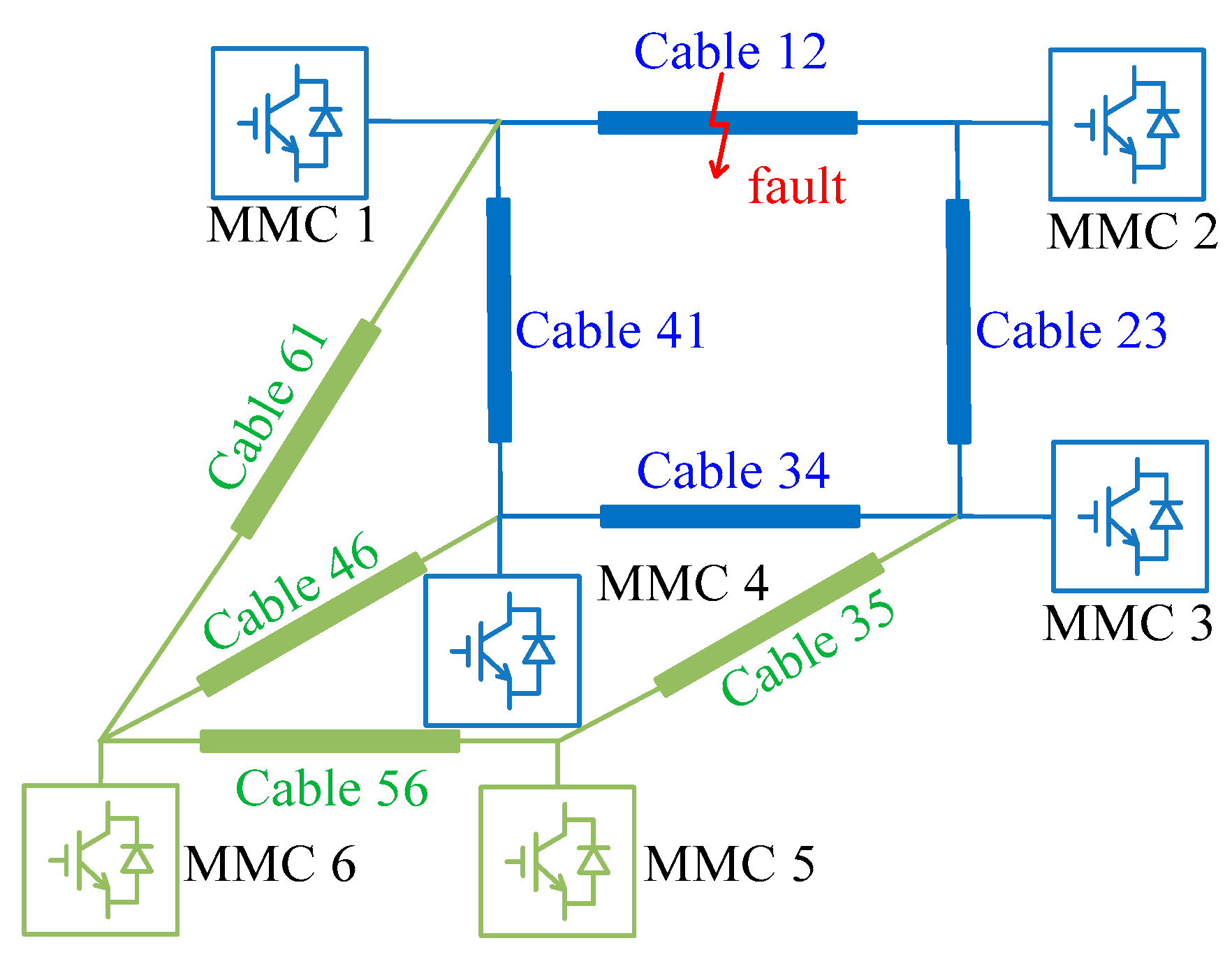
To further verify the effectiveness and universality of the above methods, a six-terminal MMC-HVDC transmission system is built on the PSCAD. The topological structure is demonstrated in Figure 10, and the parameters of the MMC and transmission line are shown in Table 5 and Table 6, respectively. When the bipolar short-circuit fault occurs on cable 12, the analytical calculation method proposed in this paper is used to obtain the current of the line. The comparison between the calculated current and the simulation one is shown in Figure 11. From this, we could learn that this method is also suitable for multi-terminal flexible HVDC systems with complex structures, and the maximum error between the short-circuit current calculated by the distributed parameter method and the simulation value within 10 ms is significantly smaller than that calculated by the lumped parameter. The correctness of the proposed calculation method is verified.
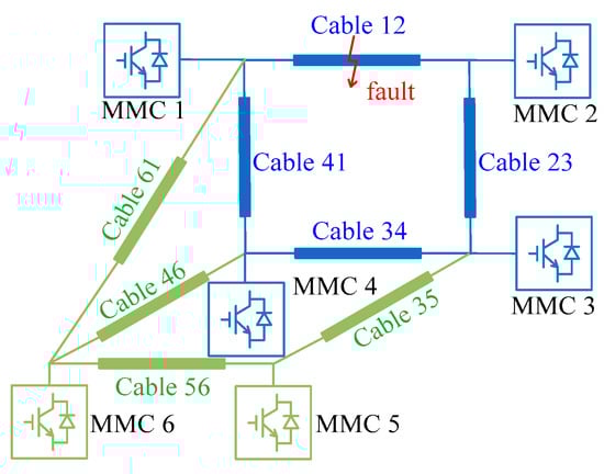
Figure 10.
Topology of six-terminal flexible HVDC system.
Table 5.
The parameters of the MMC in the six-terminal system.
Table 6.
The major parameters of the line.
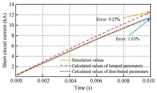
Figure 11.
Simulation and calculation comparison of six-terminal flexible HVDC system.
6. Conclusions and Limitations
The DC short-circuit analytical expression of a flexible HVDC system considering the distributed parameter model is an important component that must be configured in the development of DC power networks. In order to obtain an appropriate method for calculating the short-circuit current of long-distance transmission lines, the transmission line equation for transmission lines is first studied, the transmission line model of unit length is established, the relationship between voltage and current at both ends and line parameters is deduced, and then the line model is made approximately equivalent. A method for calculating the MMC-HVDC short-circuit current on the DC side considering the distributed parameter model for long-distance transmission lines is presented. The main conclusions are as follows:
- With an increase in the transmission line length, the error between the equivalent impedance calculated with the lumped parameter model and the equivalent impedance calculated with the distributed parameter model increases significantly. When the line length is less than 300 km, the equivalent reactance calculated with the lumped parameter model and the distributed parameter model is basically equal; when the line length exceeds 350 km, the equivalent reactance calculated with the lumped parameter model and the distributed parameter model is basically equal. The deviation in the equivalent reactance of the two models increases gradually with an increase in the line and reaches about twice the error at 1000 km.
- When the line length is less than 300 km, the lumped parameter model can be used for direct calculation; when the line length is 300–500 km, the circuit impedance is calculated with the modified coefficient method to solve the short-circuit current. When the line length is greater than 500 km, the Gorev method line equivalent model is used for calculation.
- Upon comparing the simulation and analytical calculation values for different fault distances, the results show that the analytical calculation values can better characterize the fault current characteristics and effectively reduce the error of the lumped parameter model.
Although this research found some interesting and meaningful conclusions, there are still some limitations to this study. For instance, we only studied the case of short-circuit faults in DC lines, not lightning discharge, open-circuit faults, and so on. In the future, further research can be conducted to study the effects of disturbances.
Author Contributions
Conceptualization, Z.W. (Zhuoya Wang) and L.H.; methodology, Z.W. (Zhuoya Wang); software, Z.W. (Zhuoya Wang) and Z.W. (Zemin Wang); validation, Z.W. (Zhuoya Wang); formal analysis, Z.W. (Zhuoya Wang); investigation, Z.W. (Zemin Wang); resources, L.H.; data curation, Z.W. (Zhuoya Wang); writing—original draft preparation, Z.W. (Zhuoya Wang); writing—review and editing, Z.W. (Zhuoya Wang) and Z.W. (Zemin Wang); visualization, Z.W. (Zhuoya Wang); supervision, L.H.; project administration, L.H.; funding acquisition, L.H. All authors have read and agreed to the published version of the manuscript.
Funding
This research was funded by the National Natural Science Foundation of China Key Project (grant number U2066210).
Data Availability Statement
The original contributions presented in the study are included in the article, further inquiries can be directed to the authors.
Conflicts of Interest
The authors declare no conflicts of interest.
References
- Liao, Y.; Jin, L.; You, J.; Xu, Z.; Liu, K.; Zhang, H.; Shen, Z.; Deng, F. A Novel Voltage Sensorless Estimation Method for Modular Multilevel Converters with a Model Predictive Control Strategy. Energies 2024, 17, 61. [Google Scholar] [CrossRef]
- Wang, Z.; Hao, L.; He, J. Short-circuit current calculation on DC side of MMC-HVDC system with long distance transmission lines. In Proceedings of the 2023 3rd International Conference on Electrical Engineering and Control Science (IC2ECS), Hangzhou, China, 29–31 December 2023; pp. 300–306. [Google Scholar]
- Sun, Y.; Li, Z.; Zhang, Y.; Li, Y.; Zhang, Z. A Time-Domain Virtual-Flux Based Predictive Control of Modular Multilevel Converters for Offshore Wind Energy Integration. IEEE Trans. Energy Convers. 2022, 37, 1803–1814. [Google Scholar] [CrossRef]
- Wei, N.; Zhou, N.; Liao, J.; Luo, Y.; Wang, Q. A Parameters Optimal Method for Fault Current Limiting Devices of MMC Based on Fault Current Amplitude and Energy Limiting Contribution. Proc. CSEE 2021, 41, 3751–3764. [Google Scholar]
- Hu, K.; Mao, M.; He, Z.; Cheng, D.; Lu, H. Optimization of inductance parameters of main circuit for MMCHVDC grid based on transient energy suppression under DC short-circuit faults. Proc. CSEE 2022, 42, 1680–1690. [Google Scholar]
- Wang, Z.; Hao, L.; Wang, L.; He, J. Analysis and general calculation of DC fault currents in MMC-MTDC grids. Electr. Power Syst. Res. 2023, 224, 1809–1817. [Google Scholar] [CrossRef]
- Lin, S.; Li, X.; Lei, X.; Xie, G.; He, Y. Risk Analysis and Prevention Measures of Operation Mode Transformation for Zhangbei VSC-based DC Grid. Power Sys. Technol. 2023, 47, 4017–4025. [Google Scholar]
- Li, J.; Zhang, Z.; Li, Z.; Babayomi, O. Predictive Control of Modular Multilevel Converters: Adaptive Hybrid Framework for Circulating Current and Capacitor Voltage Fluctuation Suppression. Energies 2023, 16, 5772. [Google Scholar] [CrossRef]
- Lewis, P.; Grainger, B.; Hassan, H.; Barchowsky, A.; Reed, G. Fault Section Identification Protection Algorithm for Modular Multilevel Converter Based High Voltage DC with a Hybrid Transmission Corridor. IEEE Trans. Ind. Electron. 2016, 63, 5652–5662. [Google Scholar] [CrossRef]
- Deng, F.; Tian, Y.; Zhu, R.; Chen, Z. Fault-Tolerant Approach for Modular Multilevel Converters Under Submodule Faults. IEEE Trans. Ind. Electron. 2016, 63, 7253–7263. [Google Scholar] [CrossRef]
- Wang, Z.; Hao, L.; He, J. Research on Influence Factors in MMC-HVDC Short-Circuit Current Based on Improved Calculation Method. In Proceedings of the 2023 The 8th International Conference on Power and Renewable Energy (ICPRE), Shanghai, China, 22–25 September 2023; pp. 44–50. [Google Scholar]
- Li, B.; Zhou, S.; Xu, D.; Yang, R.; Xu, D.; Buccella, C.; Cecati, C. An Improved Circulating Current Injection Method for Modular Multilevel Converters in Variable-Speed Drives. IEEE Trans. Ind. Electron. 2016, 63, 7215–7225. [Google Scholar] [CrossRef]
- Zhang, Z.; Xu, Z. Short-circuit current calculation and performance requirement of HVDC breakers for MMC-MTDC systems. IEEJ Trans. Electr. Electron. Eng. 2016, 11, 168–177. [Google Scholar] [CrossRef]
- Wang, Z.; Hao, L.; Wang, L.; He, J. Calculation method of nonmetallic fault short circuit current in DC side of MMC-HVDC. Electr. Power Auto Equip. 2024, 44, 187–194. [Google Scholar]
- Li, M.; Luo, Y.; He, J.; Zhang, Y.; Meliopoulos, A. Analytical estimation of MMC short-circuit currents in the AC in-feed steady-state stage. IEEE Trans. Power Deliv. 2021, 37, 431–441. [Google Scholar] [CrossRef]
- Han, X.; Sima, W.; Yang, M.; Li, L.; Yuan, T.; Si, Y. Transient Characteristics Under Ground and Short-circuit Faults in a ±500 kV MMC-Based HVDC System with Hybrid DC Circuit Breakers. IEEE Trans. Power Deliv. 2018, 33, 1378–1387. [Google Scholar] [CrossRef]
- Xu, J.; Zhu, S.; Li, C.; Zhao, C. The Enhanced DC Fault Current Calculation Method of MMC-HVDC Grid with FCLs. IEEE J. Emerg. Sel. Top. Power Electron. 2019, 7, 1758–1767. [Google Scholar] [CrossRef]
- Li, C.; Zhao, C.; Xu, J.; Ji, Y.; Zhang, F. A Pole-to-pole short-circuit fault current calculation method for DC grids. IEEE Trans. Power Syst. 2017, 32, 4943–4953. [Google Scholar] [CrossRef]
- Langwasser, M.; Giobanni, D.; Liserre, M.; Biskoping, M. Improved Fault Current Calculation Method for Pole-to-Pole Faults in MMC Multi-Terminal HVDC Grids Considering Control Dynamics. In Proceedings of the 2018 IEEE Energy Conversion Congress and Exposition (ECCE), Portland, OR, USA, 23–27 September 2018. [Google Scholar]
- Langwasser, M.; Giobanni, D.; Liserre, M.; Biskoping, M. Fault Current Estimation in Multi-Terminal HVDC Grids Considering MMC Control. IEEE Trans. Power Syst. 2019, 34, 2179–2189. [Google Scholar] [CrossRef]
- Torwelle, P.; Bertinato, A.; Raison, B.; Le, T.; Petit, M. Fault current calculation in MTDC grids considering MMC blocking. Electr. Power Syst. Res. 2022, 207, 1–12. [Google Scholar] [CrossRef]
- Sun, P.; Jiao, Z.; Gu, H. Calculation of Short-Circuit Current in DC Distribution System Based on MMC Linearization. Front. Energy Res. 2021, 9, 634232. [Google Scholar] [CrossRef]
- Gu, J.; Hu, J.; Jiang, L.; Wang, Z.; Zhang, X.; Xu, Y.; Zhu, J.; Fang, L. Research on Object Detection of Overhead Transmission Lines Based on Optimized YOLOv5s. Energies 2023, 16, 2706. [Google Scholar] [CrossRef]
- Man, J.; Xie, X.; Tang, J.; Wang, Y.; Luo, Y. Transmission line modeling for high frequency resonance analysis of MMC-HVDC systems. Power Syst. Technol. 2021, 45, 1782–1789. [Google Scholar]
- Li, Z.; Dai, Z.; Shi, X.; Yang, M. Approximate Calculation Method of Short-Circuit Current of Multi-Terminal Hybrid DC Transmission System Considering Control Strategy. Trans. China Electrotechnol. Soc. 2024, 39, 2810–2824. [Google Scholar]
- Souza, N.; Carvalho, C.; Kurokawa, S.; Pissolato, J. A Distributed-parameters Transmission Line Model Developed Directly in the Phase Domain. Electr. Mach. Power Syst. 2013, 41, 1100–1113. [Google Scholar] [CrossRef]
- Xie, R.; Zhang, G.; Xie, B. Analysis and Suppression of Harmonic Instability for Grid-connected Inverter System Considering Characteristics of Long Transmission Cable. Auto Electr. Power Syst. 2024, 48, 128–139. [Google Scholar]
- Ma, J.; Shi, Y.; Ma, W.; Wang, Z. Location Method for Interline and Grounded Faults of Double-Circuit Transmission Lines Based on Distributed Parameters. IEEE Trans. Power Deliv. 2015, 30, 1307–1316. [Google Scholar] [CrossRef]
- Nie, Y.; Liu, Y.; Pan, R.; Lu, D.; Fan, R. Convolution Based Time Domain Fault Location Method for Lines in MMC-HVDC Grids with Distributed and Frequency Dependent Line Model. IEEE Trans. Power Deliv. 2023, 38, 3860–3874. [Google Scholar] [CrossRef]


Disclaimer/Publisher’s Note: The statements, opinions and data contained in all publications are solely those of the individual author(s) and contributor(s) and not of MDPI and/or the editor(s). MDPI and/or the editor(s) disclaim responsibility for any injury to people or property resulting from any ideas, methods, instructions or products referred to in the content. |
© 2024 by the authors. Licensee MDPI, Basel, Switzerland. This article is an open access article distributed under the terms and conditions of the Creative Commons Attribution (CC BY) license (https://creativecommons.org/licenses/by/4.0/).