Abstract
Subsynchronous oscillations have occurred in wind farms due to the high penetration of converter-based technology in power systems and may potentially lead to grid instability. As an effective solution, synchronous condensers, with their ability to control voltage and inject reactive power in the power system, are increasingly being adopted, as they can lead to the mitigation of such oscillations in weak grid conditions. However, the impact of synchronous condensers’ power ratings on system stability is a topic that requires further investigation. In fact, an improper selection of a synchronous condenser’s rating will not extinguish existing subsynchronous oscillations and may even cause the emergence of new oscillatory phenomena. This paper presents a novel examination of the impact that the synchronous condenser’s power rating has on the small-signal stability of a wind farm with existing subsynchronous oscillations while being connected to a weak grid. The wind farm’s model is developed using state-space modeling, centering on grid interconnection and incorporating the state-space submodel of a synchronous condenser to show its impact on subsynchronous oscillation mitigation. The stability analysis determines the optimal synchronous condenser’s power ratings for suppressing these oscillations in the wind farm model. The findings are corroborated through time domain simulations and fast-Fourier transformation (FFT) analysis, which further validate the stability effects of a synchronous condenser’s rating.
1. Introduction
The utilization of renewable energy has experienced significant growth in recent years. According to the latest Renewables Global Status Report (GSR) by the Renewable Energy Policy Network for the 21st Century (REN21), renewables accounted for 29.9% of global electricity generation in 2022, an increase from 28.3% in 2021 and a notable increase from 21.3% in 2012. Although fossil fuels still dominate in meeting the global energy demand, their share has decreased from 68% in 2012 to 61% in 2022 [1]. In terms of wind energy capacity, there was a global addition of 599 GW in onshore and offshore wind installations from 2014 to 2022. The year 2022 marked the third best year for new capacity, with 75 GW added globally, according to the latest report by the International Renewable Energy Agency (IRENA) [2]. Between 2023 and 2027, an expected 680 GW of new wind capacity is projected to be installed, with 130 GW of this capacity being offshore, as per the Global Wind Energy Council (GWEC) [3].
To accommodate this large-scale generation of wind energy, power electronic technology has been widely adopted, leading to a shift from traditional synchronous machine-based power grids to converter-based power grids. This transition has brought an increased flexibility and also, in cases, improved efficiency for the grid [4]. On the other hand, this transformation has given stability challenges, particularly in weak grid conditions, due to control interactions in the converter-based power system. Additionally, during periods of high instantaneous wind penetration, when fewer synchronous generators are online, frequency stability may be compromised due to reduced governor response, especially in smaller systems with reduced synchronous inertia [5].
Such conditions can lead to subsynchronous oscillations (SSO), which arise in wind farms and grid systems, posing a significant threat to the normal operation of the wind farm [6]. The interest in SSOs in wind farms has been increased in the last 15 years, due to an incident that involved a sustained oscillation phenomenon in Texas’s Southern power grid. The oscillation frequency was lower than the synchronous frequency (equal to 20 Hz) and was triggered by a line fault. A similar phenomenon also occurred in the Buffalo Ridge area of Minnesota [7,8]. Therefore, the analysis of subsynchronous oscillation phenomena has become a crucial topic for the stability of wind farm systems in recent years.
The mitigating measures utilized in order to deal with SSOs in wind farms are categorized in control and hardware solutions. The software solutions for mitigating SSOs include the tuning of converter controller parameters, digital filters, and supplementary damping controller (SDC), as well as the utilization of grid-forming control concepts. The hardware solutions for mitigating SSOs often involve installing additional equipment in the grid of the system operator. These solutions, as explained in [7], rely on flexible AC transmission system (FACTS) devices such as static var compensators (SVC) and static synchronous compensators (STATCOM).
Synchronous condensers (SC) have gained renewed popularity in recent years as a mitigating measure of SSOs due to their ability to provide voltage control and inject reactive power simultaneously [9,10]. SCs are synchronous machines that do not generate electricity but only spin freely without a prime mover. By regulating their field voltage, SCs can control their reactive power exchange with the grid, thereby strengthening the network to which they are connected [11]. Specifically, when an SC is connected to the grid, the equivalent impedance viewed from the point of commoncoupling (PCC) decreases, which can influence the system stability, whereas a STATCOM without an additional damping controller may not have the same impact on impedance. SCs can improve system damping in doubly-fed induction generator (DFIG) and permanent magnet synchronous generator (PMSG) systems. Furthermore, unlike other mitigation measures, SCs can mitigate SSOs without requiring any upgrades or extra damping controllers [12].
Several studies have been applied regarding the impact of SCs as a mitigating measure for SSOs. There have been many studies where the advantage of SC has been highlighted compared to other hardware solutions like STATCOM and SVC; this issue has been addressed in [12,13,14]. In [15,16], the combined effect of the control strategies in a converter-based power system with SC is under analysis. Optimization techniques for the optimal allocation of the synchronous condenser within the grid, as well the formulation of the cost and sizing have been investigated in [11,17,18,19]. A practical application of SC has been successfully implemented in the Australian power grid [20], where its usage demonstrated a significant positive effect by mitigating SSOs and effectively integrating renewable energy sources better.
However, prior studies have not explored how SCs with varying power ratings can effectively mitigate existing SSOs after an SC is incorporated into a wind farm. Indeed, the significance of the SC power rating, as well as the determination of its optimal upper and lower limits for effectively dealing with SSOs, have been insufficiently explored. In case the SC connected to the wind farm system has a rating below the identified optimal lower limit, the existing SSOs will not be mitigated successfully; similarly, if the SC connected to the wind farm system has a rating above the identified optimal upper limit, then low-frequency dynamics are reintroduced to the system. This study aims to highlight the crucial role that SCs with different power ratings can play in mitigating these instabilities in wind farms.
In this paper, an analytical small-signal model of a wind farm based on the HVAC CIGRE benchmark model [6] is first developed and validated by applying eigenvalue analysis of its controllers; thus, the state-space sub-model of the synchronous condenser can be included after also being validated. The impact of the SC rating in attenuating successfully existing SSOs in weak-grid conditions is highlighted. The paper’s novelty lies in the identified optimal range of the SC power ratings, where the system under study can successfully deal with unwanted dynamic phenomena in the subsynchronous resonance frequency range for weak grids. In case the SC’s rating is out of this range, the stability of the system will not be possible to obtain.
2. Small-Signal Model of Wind Farm
2.1. Small-Signal Modeling
Converters exhibit time-varying and nonlinear behavior due to switching modulation and variable duty cycles within their closed-loop control, resulting in their operation being nonlinear and time-varying [4]. As a result, they introduce small-signal dynamics to the wind farm that may lead to resonances and harmonic phenomena. To pinpoint the causes of small-signal instability in modern converter-based power systems that penetrate wind power, it is necessary to develop linearized models of power converters [6]. Small-signal stability refers to the ability of a converter-based system to return to a steady state after minor disturbances. Impedance-based stability analysis and eigenvalue-based stability analysis are widely used techniques for analyzing small-signal stability in converter-based power systems [21].
Impedance-based modeling involves creating equivalent impedance models that represent the interactions between the converter and the grid at the PCC. These impedance models determine the open-loop gain of the system and stability is assessed using the Nyquist stability criterion [6,21]. On the other hand, eigenvalue-based modeling provides a comprehensive analysis of the system dynamics by utilizing a state-space representation, which allows for modal analysis of the system. The nonlinear model is linearized around an equilibrium point and the eigenvalues of the state matrix indicate the system’s stability [6]. Here, a state-space model is employed to investigate the small-signal stability of a wind farm and the focus will be on SSOs.
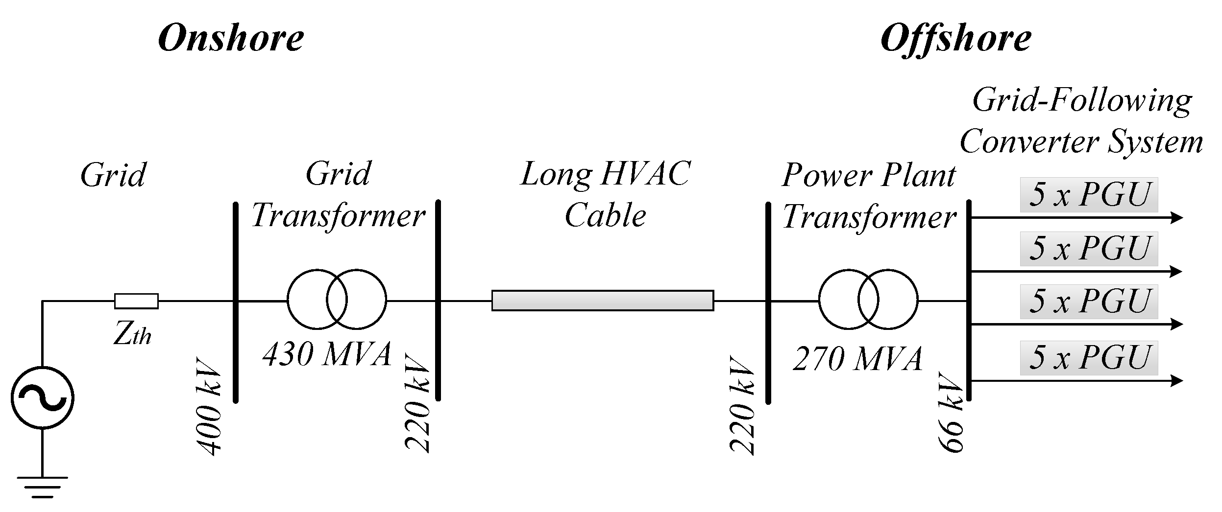
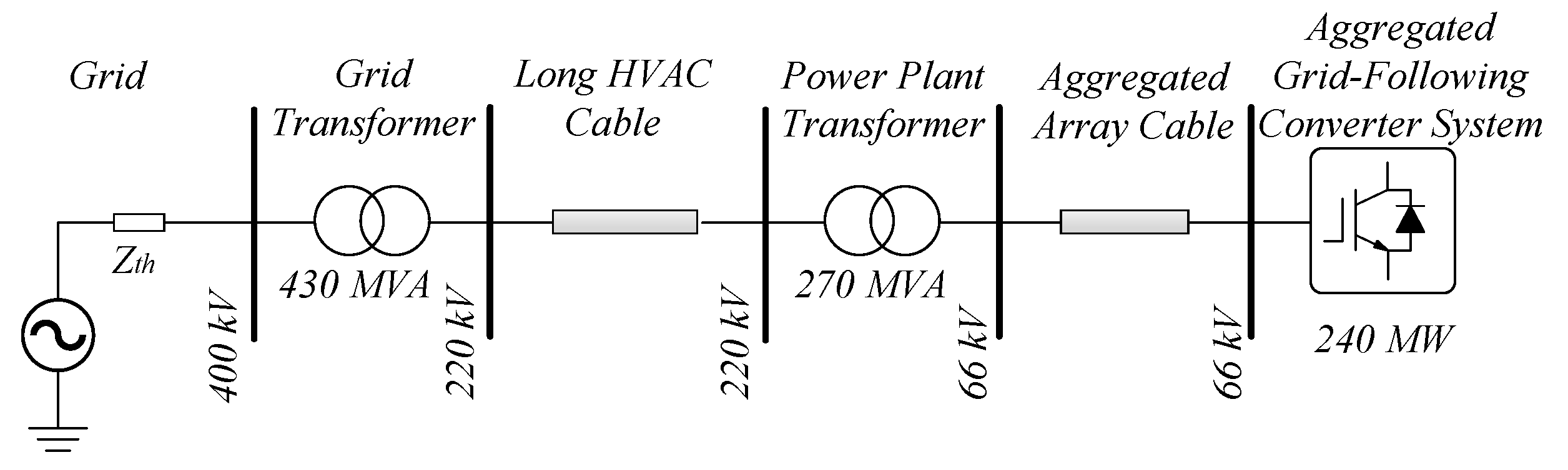
The case examined is based on the HVAC CIGRE benchmark model of a wind farm [6]. This model is an outcome of the work conducted in the CIGRE working group C4.49 entitled “Multi-frequency stability of converter-based modern power systems” and the main objective of the benchmark power system is to provide a reference system where converter-to-converter as well as converter-to-grid interactions can be investigated. The model considers aggregated power generation units (PGUs) connected to an AC power grid; in fact, PGUs of 240 MW and −4 × 5 PGUs of 12 MW in total, are utilized in the developed small-signal model as presented in Figure 1; the equivalent structure with the aggregated grid-following converter control is shown in Figure 2.

Figure 1.
All power generation units (PGUs) in a wind farm, connected to a Thevenin equivalent grid.
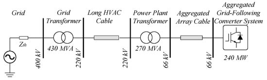
Figure 2.
Aggregated grid following converters connected to a Thevenin equivalent grid with cables and transformers in between.
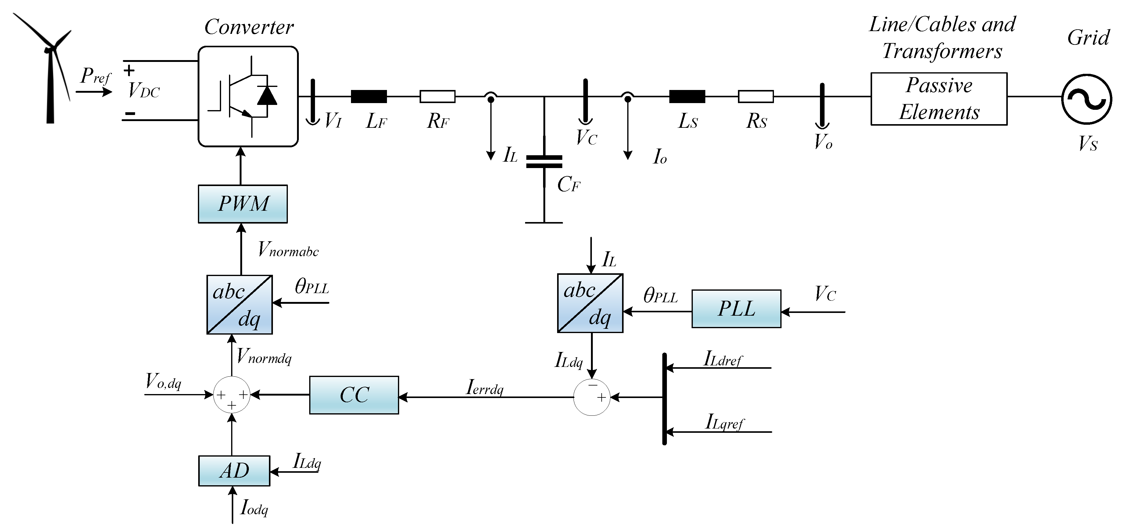
2.2. Wind Turbine’s Grid-Connected Voltage-Source Converter (VSC)
The aggregated wind turbine model utilizes the control structure depicted in Figure 3, and can be applied to both Type-3 and Type-4 wind turbines. For simplicity, the mechanical system of the wind turbines is not considered in this analysis. The philosophy of the converter control structure is inherited from [22], where the model entails a grid-following converter, which adopts vector current control (CC). An active damping (AD) control is added in order to enhance the system’s stability when dealing with weak or highly dynamic grids. The synchronization of the converter to the grid is achieved by a phase-locked loop (PLL), where the grid and the control dq frame are defined and utilized; this is analytically explained in [23]. An ideal converter is assumed, where the DC link voltage of the inverter is assumed to be constant and the reference output current is set as default; therefore, the outer-loop control is not considered for simplification and the reference currents in the dq− axis are input variables of the wind farm’s state-space model.
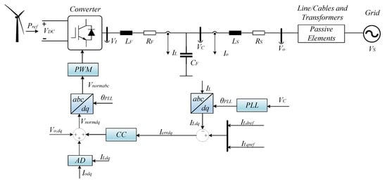
Figure 3.
Control structure of an aggregated wind turbine model with a grid-following converter applying a PLL for synchronization.
2.3. Passive Elements
The passive elements between the VSC and the grid consist of cables, transmission lines, and step-up transformers.
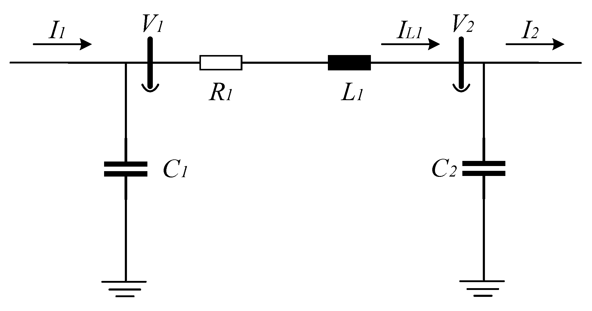
2.3.1. Transmission Line and Cable Modeling
Lines and cables are of vital importance, as they represent an important share of the system impedance. The main difference between them is that cables have a capacitance that pushes the system resonance to lower frequencies [24]. In both cases, a nominal pi model is utilized in their state-space representation, which is shown in Figure 4. When the transmission line is modeled, a sufficient number of pi-sections is utilized, as the modelling accuracy of the transmission line is improved by increasing the number of nominal pi sections.

Figure 4.
The nominal pi-section utilized for cable and transmission line modeling (passive elements in Figure 3).
Two types of collection cables are used; the 500 mm2 3-core cable and the 150 mm2 3-core cable. In each cable string, there are five PGUs. The 500 mm2 3-core cable is used for the first three PGUs and the 150 mm2 3-core cable is used for the last two PGUs. The cable length between the PGUs in the cable string is equal to 5 km. Regarding the transmission cable, 10 pi-sections of the 1200 mm2 HVAC cable are utilized to formulate it [6]. The corresponding cable parameters are shown in Appendix A.
The state equations that correspond to the nominal pi in dq domain are given below as follows:
2.3.2. Transformer Model
Transformer is a passive element that allows the transfer of power to very long distances due to the magnetic coupling between different voltage levels; its classical model is depicted in Figure 5.
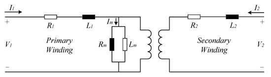
Figure 5.
Classical transformer equivalent model with lumped parameters (passive elements in Figure 3).
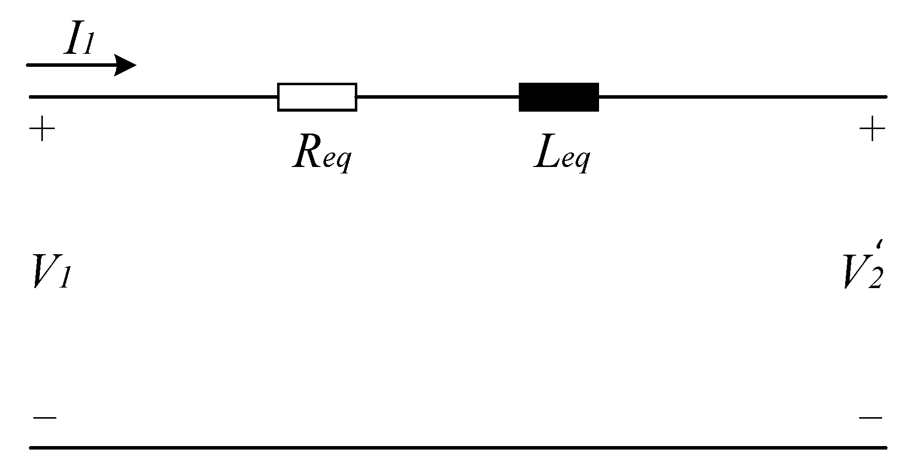
Since the magnetization inductance is quite large, the exciting current drawn by the magnetizing branch will be very small. Therefore, the magnetizing branch can be neglected and the winding resistances and reactances, which are now in series, can be combined into equivalent resistance and reactance of the transformer as seen from the appropriate side. The equivalent circuit of the transformer, where the transformer’s elements are referred to the primary side, is shown in Figure 6.

Figure 6.
Transformer equivalent model reflected to one voltage level after neglecting the magnetizing branch.
The state equations of the transformer’s equivalent model are given below as follows:
where is the secondary terminal voltage of the transformer referred to the primary side on the dq axis.
To optimize the power transmission from the wind farm to shore, the voltage is stepped up in multiple steps from 0.69 kV at the wind turbine terminals to the typical grid connection point at a nominal voltage of 400 kV. In addition, the step-up transformer of the SC is similarly modeled in order to step up the voltage from 26 kV to 220 kV. The corresponding transformer parameters are shown in Appendix A.
2.4. Wind Farm Model Accuracy using Eigenvalue-Based Stability Analysis
The eigenvalue-based stability analysis using small-signal models is presented for the aggregated wind turbine model’s controllers from Figure 3 in order to study their accuracy. This is a necessary procedure in order to incorporate the state-space submodel of the SC into a validated wind farm model. The corresponding system and control parameters of the converter system are shown in Appendix A. The design target of the PI current controllers is to obtain a bandwidth of the current closed loop at around 1/20 of the switching frequency. The PLL’s bandwidth is intentionally set at a lower frequency of 11.95 Hz to minimize potential distortions caused by high-order harmonics on the PLL’s output signals.
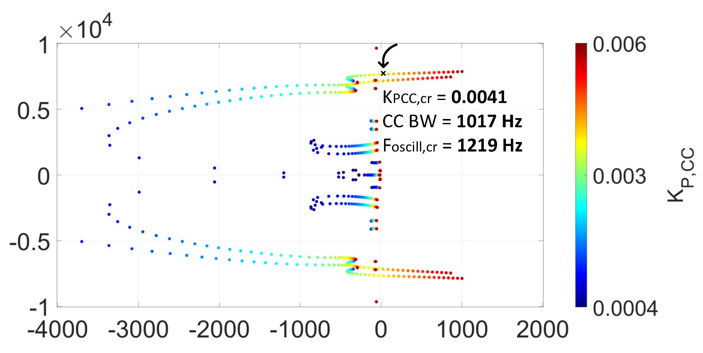
2.4.1. Eigenvalue Analysis for the Current Controller’s Control Parameters
The CC’s sensitivity is first studied. The controller gains are varied from 1 (deep blue) to 15 (red) times the default value of the controller. The eigenvalues pair of instability values are shown in Figure 7, where the corresponding critical gain , critical oscillation frequency and controller’s bandwidth are underlined. Based on the movements of the eigenvalue trajectories, the system becomes unstable as the proportional gain of the CC increases.
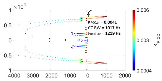
Figure 7.
Eigenvalue−based stability analysis: trajectories for CC’s proportional gain are shown.
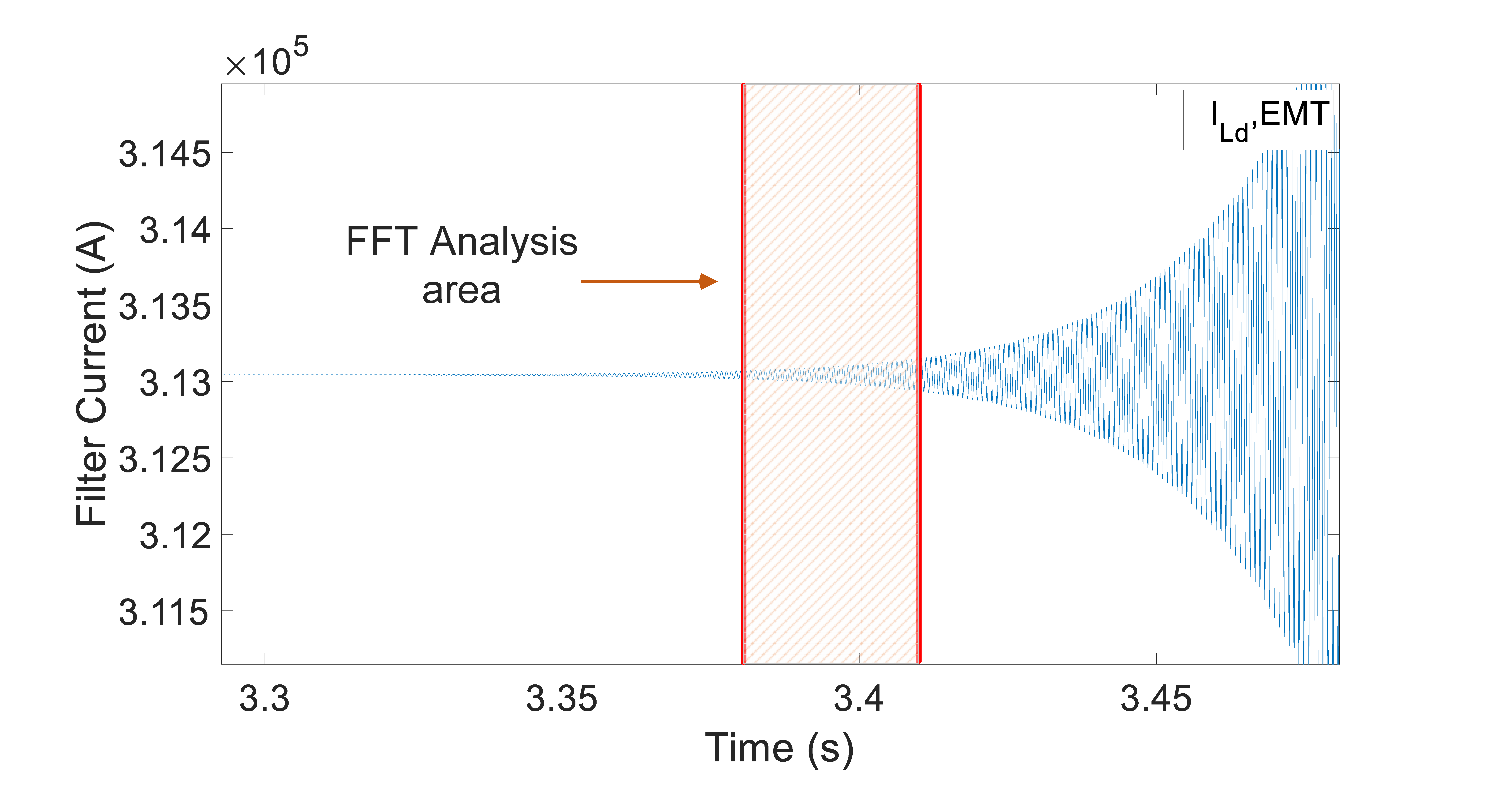
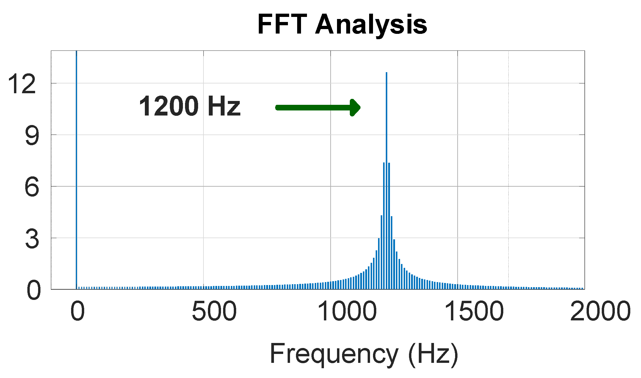
To verify the small-signal model’s dynamic response, electromagnetic transient (EMT) simulations are carried out using MATLAB Simulink R2020b. A step change was applied to the default proportional gain of the CC at s, when the system was stable initially. The controller’s gain then obtained the value that critically impacted the system’s stability () and the filter current in the dq frame was utilized to demonstrate the instability case. These simulation results are shown in Figure 8 and Figure 9, where the and the corresponding dominant oscillation frequency obtained from the FFT analysis ( Hz) are presented. It can be seen that the time domain–simulation results almost completely match with the eigenvalue analysis of the CC.
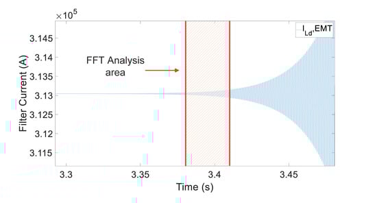
Figure 8.
Time domain simulations of the filter current when = at s.
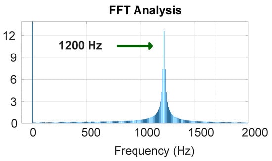
Figure 9.
FFT analysis of the filter current when = at s (see Figure 8).
2.4.2. Eigenvalue Analysis for PLL’s Control Parameters
Then, the sensitivity of the PLL is analyzed. The controller gains are varied from 0.1 (deep blue) to 10 (red) times the default value of the controller. The eigenvalues pair of instability values are shown in Figure 10, where the corresponding critical gain , critical oscillation frequency , and controller’s bandwidth are underlined. Based on the eigenvalue analysis results, the system becomes unstable as the proportional gain of the PLL increases.
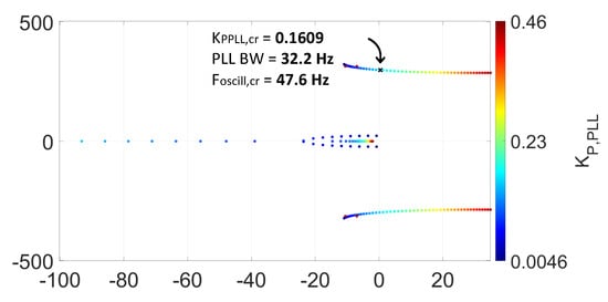
Figure 10.
Eigenvalue−based stability analysis: trajectories for PLL’s proportional gain are shown.
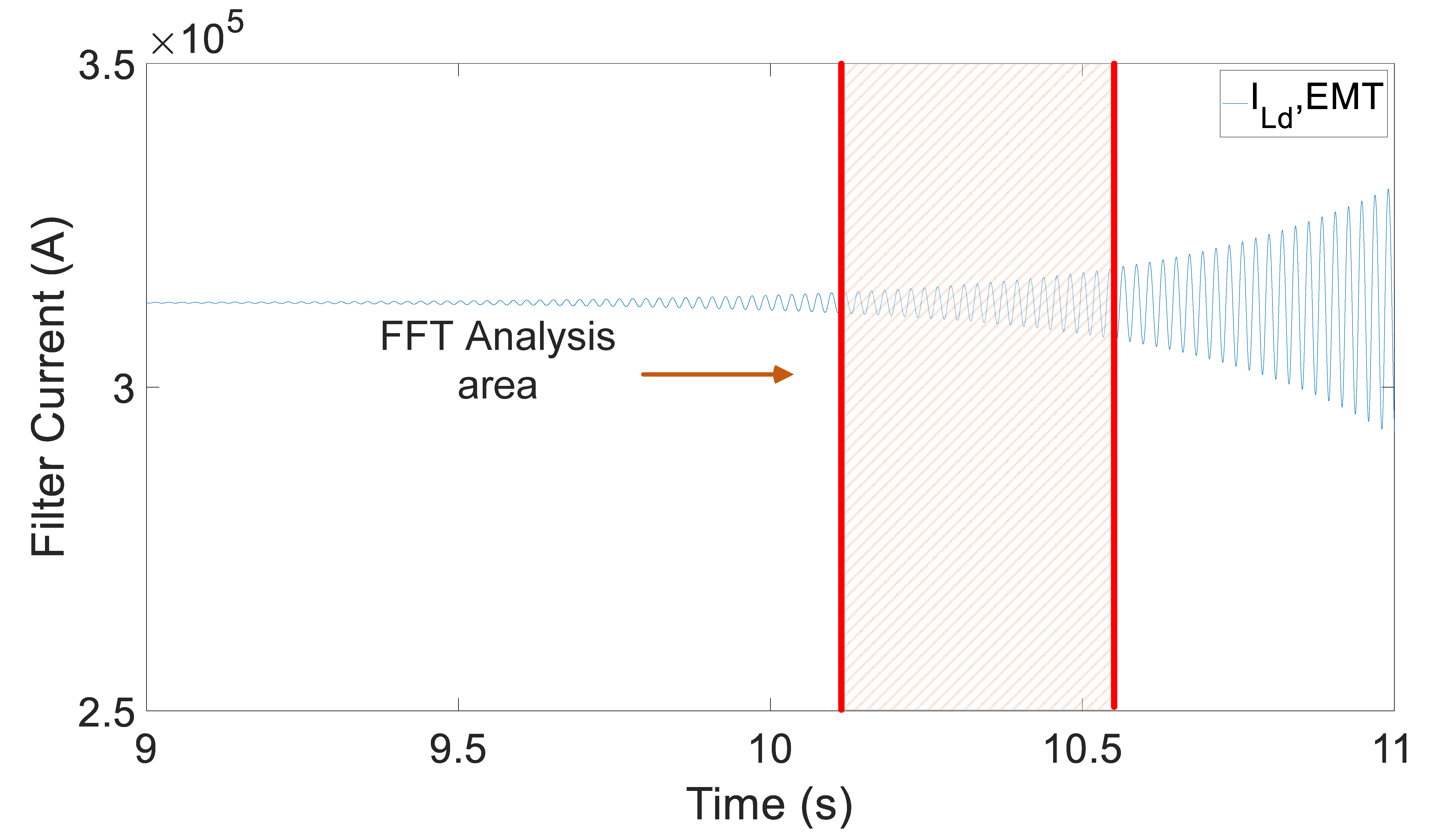
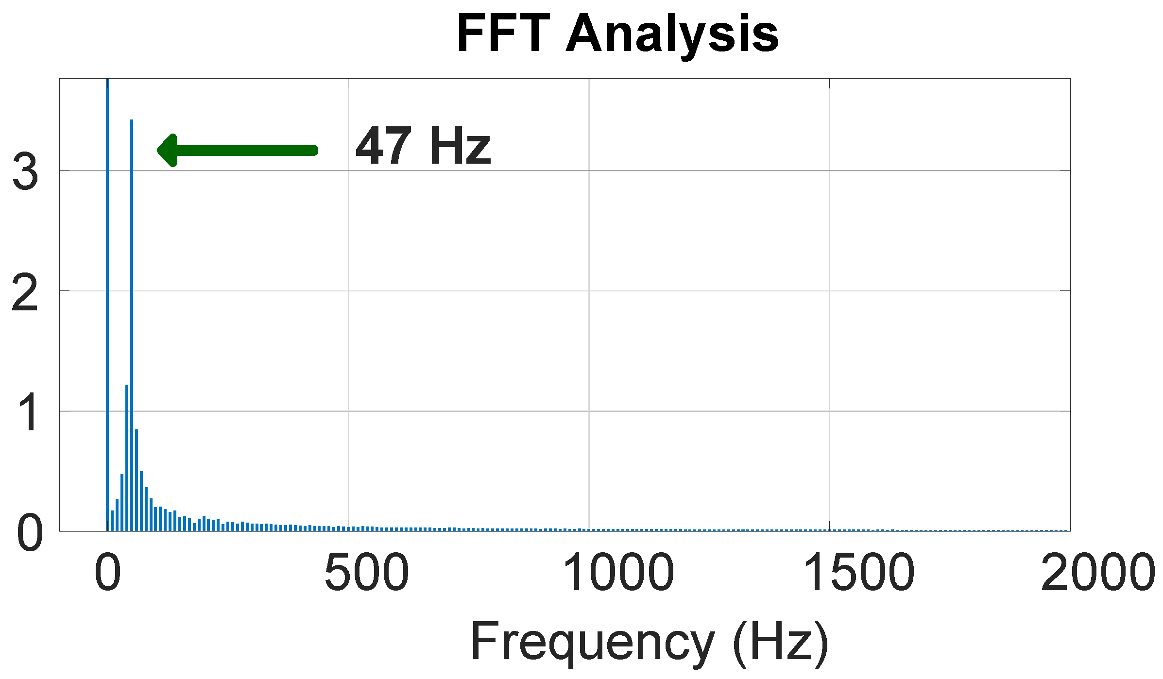
To verify the small-signal model dynamic response, EMT simulations are carried out. A step change was applied to the default proportional gain of the PLL at s, when the system was stable. The controller’s gain then obtained the value that critically impacted the system’s stability () and the filter current in the dq frame was utilized to demonstrate the instability case. These simulation results are shown in Figure 11 and Figure 12, where the and the corresponding dominant oscillation frequency obtained from the FFT analysis ( Hz) are presented. Again, the time domain–simulation results almost completely match with the eigenvalue analysis of the PLL.
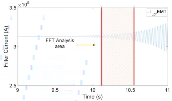
Figure 11.
Time domain simulations of the filter current when = at s.
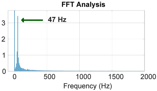
Figure 12.
FFT analysis of the filter current when = at s (see Figure 11).
Therefore, the wind farm’s small-signal model accuracy allows the inclusion of the SC state-space submodel.
3. Stability Analysis of a Synchronous Condenser
3.1. State-Space Model of a Synchronous Condenser
The SC is a type of wound-rotor synchronous machine that operates without a mechanical drive train, meaning without a prime mover attached. Consequently, the SC is unable to generate active power and the mechanical torque is equal to zero but it can control reactive power by regulating its excitation.
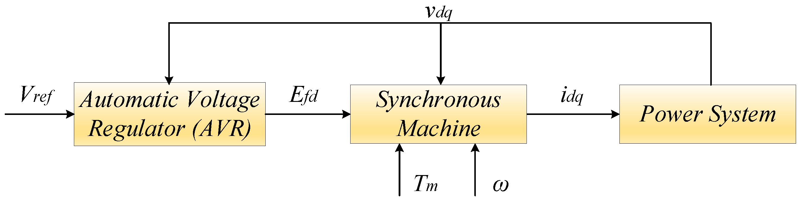
The state-space model of the SC consists of the synchronous generator state-space sub-model and the automatic-voltage regulator (AVR) state-space submodel. Figure 13 shows the system diagram of the SC and how it is model-wise-connected to the power system. The parameters of the synchronous generator are expressed in the per unit (pu) system, where the base value is the power rating of the generator . Therefore, their value in the international system of units (SI) is always dependent on . The parameters of the synchronous generator in the pu system and the AVR, which are shown in the figures and equations of Section 3.1, are defined in the Appendix B, where is varied depending on the test cases demonstrated in the following sections.
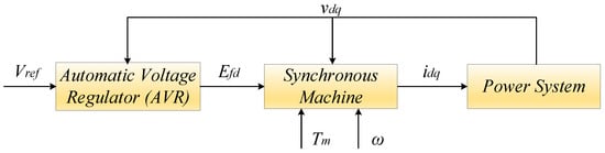
Figure 13.
System diagram of a synchronous condenser connected to a power system that includes a grid-connected offshore wind farm.
The detailed models of the synchronous machine and the AVR are analytically presented in Section 3.1.1 and Section 3.1.2.
3.1.1. Synchronous Generator Model
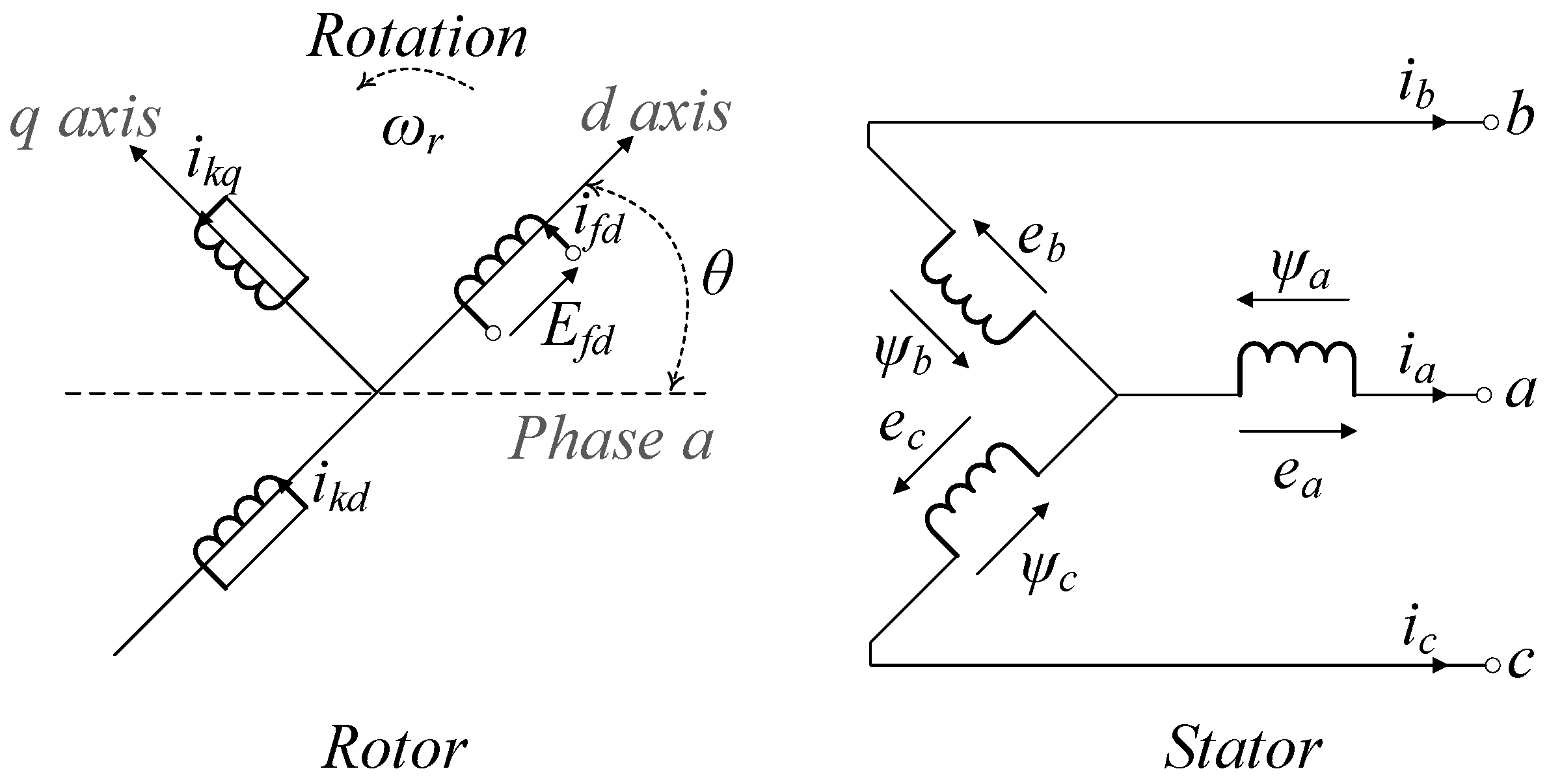
The main windings are the stator and field windings. A set of damper windings are also present in the rotor, where no current is flowing during the steady state. The field winding is aligned with the d-axis for this derivation, while the d- and q-axis damper winding circuits are present in the rotor. The dynamic behavior of the synchronous machine is defined by the magnetic couplings between the windings represented by the internal inductances [25]. Figure 14 shows the structure of the synchronous machine.

Figure 14.
Electrical model of the synchronous generator, shown in Figure 13, with rotor and stator windings including its excitation.
Based on Figure 14, the rotor windings are aligned with the d-axis. The overall flux linkage equations of the synchronous machine in the dq-frame are given below.
The voltage equations of the synchronous machine—stator voltages, field voltage and rotor voltages—are shown below:
From the voltage equations, the state-space submodel of the synchronous generator can be derived. First, the synchronous generator currents have to be expressed by utilizing (9) as
Then, (16)–(20) can be substituted into (10)–(14) and the state equations of the flux linkages are derived. The expression is defined and utilized for simplicity, where i and j refer to the row and column of (9), respectively, as follows:
Besides the state equations of the flux linkages, the equation of motion also needs to be included, as well as the state equation of angle in order to interface the grid and the SC dq-frames.
Therefore, based on [26], the overall linearized state-space model of the synchronous generator that describes its dynamics is
where
and the steady-state flux linkages are obtained by (32)–(33), as follows:
The steady-state operating points of the synchronous machine voltage and current are equal to 1 pu.
3.1.2. Automatic Voltage Regulator (AVR) Model
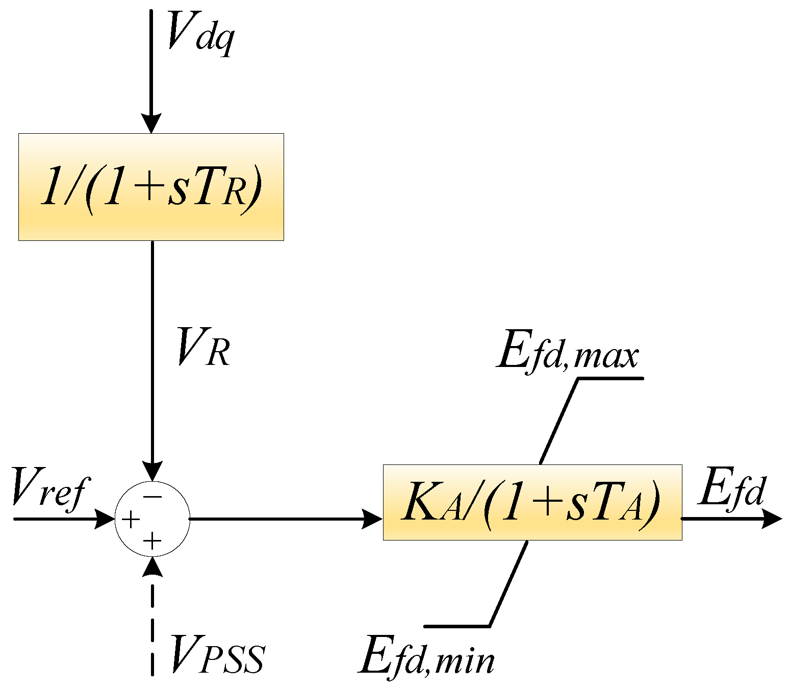
The field-voltage is regulated by the AVR based on the voltage at a selected bus enabling the synchronous machine to be used for voltage and reactive power control in the system. The voltage amplitude is input to the AVR and smoothed by a first order filter in the transducer. Figure 15 shows the structure of the AVR.

The state variables are and and the corresponding state equations are shown below:
3.2. Modeling Validation
In order to validate the small-signal model of the SC, a small external system is developed, whose parameters are shown in Table 1, and the SC described in Table A5 with a machine rating equal to 100 kVA is connected to it as shown in Figure 16. The state equations that correspond to the electrical elements of the external system follow the same concept as described in Section 2 and the connection of the SC is performed via the component–connection method (CCM).

Table 1.
System parameters of the external system for validating the synchronous condenser model.
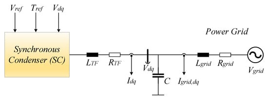
Figure 16.
SC connected to external power system for validation.
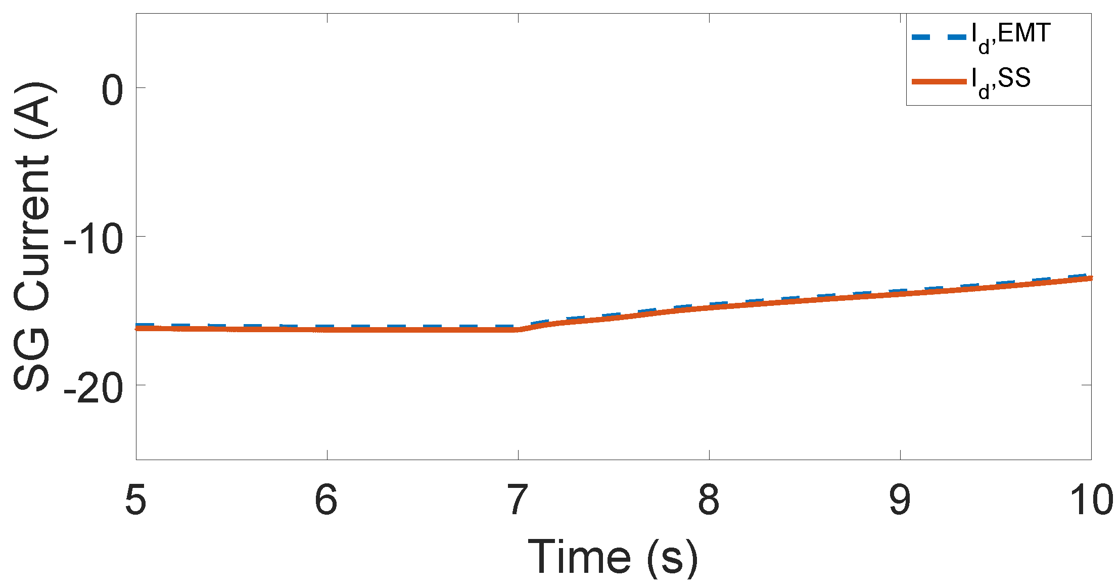
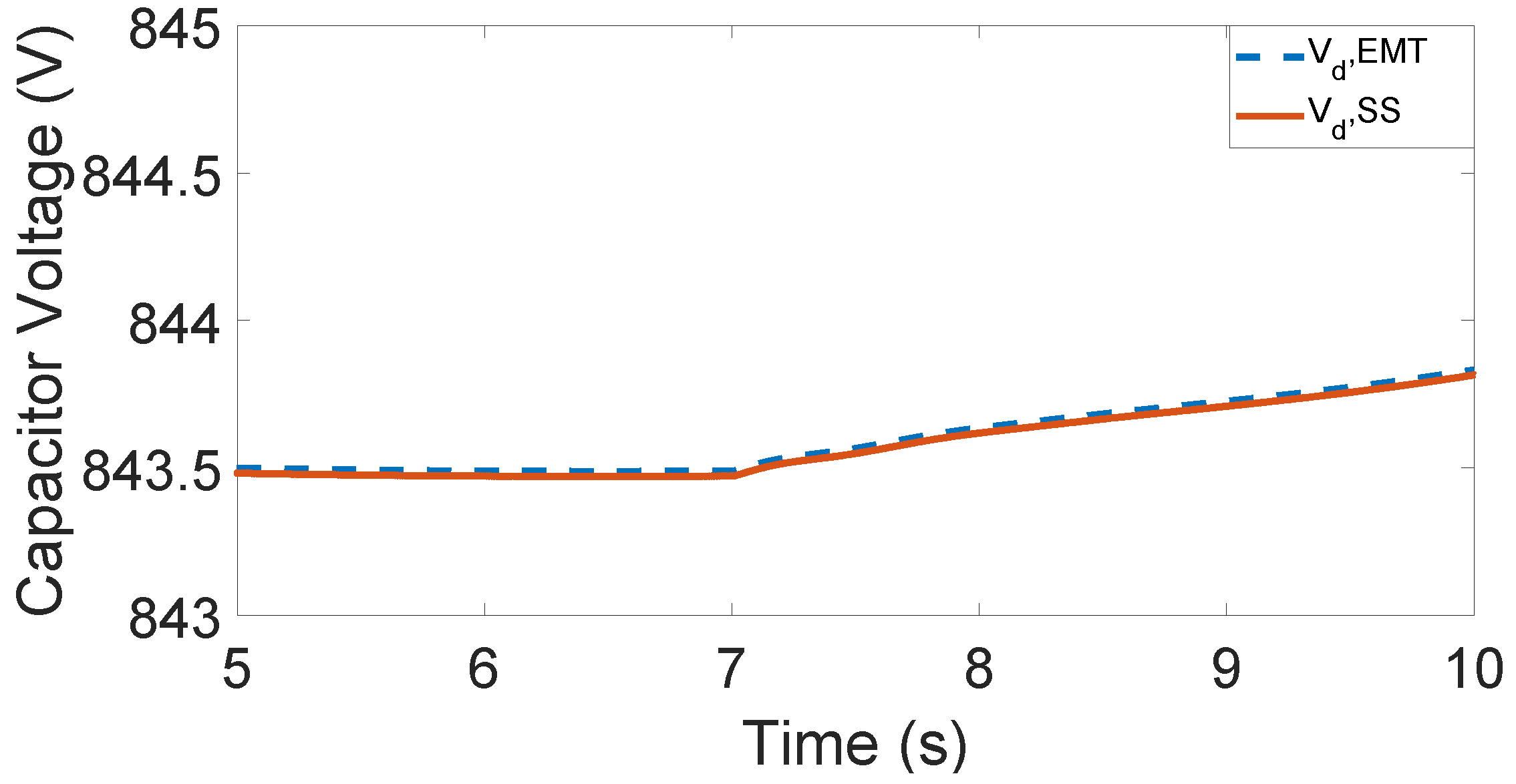
The validation procedure is implemented after performing a small step in the input reference voltage of the SC from 1 pu to 1.05 pu at s. The EMT simulation is then compared with a state-space (SS) response. As shown in Figure 17 and Figure 18, the simulation results of EMT and SS, regarding the current and the voltage , are almost the same after the small disturbance at . Therefore, the SC’s small-signal model can be integrated into the wind farm’s validated model in Section 2.4 and utilized for the stability analysis.
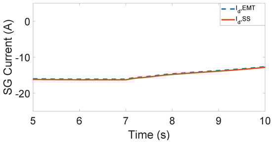
Figure 17.
Current of the external power system under a step change in reference voltage of the SC.
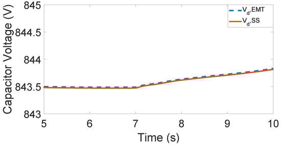
Figure 18.
Voltage of the external power system under a step change in reference voltage of the SC.
4. Stability Impact of a Synchronous Condenser’s Rating
With the validation of the small-signal model of the SC, it becomes feasible to integrate it into the small-signal model of the HVAC CIGRE benchmark model, which was described and validated in Section 2. In the HVAC CIGRE benchmark model, the SC is installed at the onshore substation through a step-up transformer, as depicted in Figure 19. The synchronous condenser’s electrical parameters are expressed in the pu system, where the SC power rating is the base value, as already mentioned in Section 3.1.
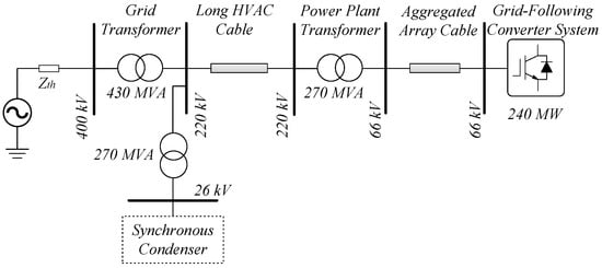
Figure 19.
HVAC CIGRE power system with 240 MW wind power plant and a synchronous condenser connected to the onshore substation.
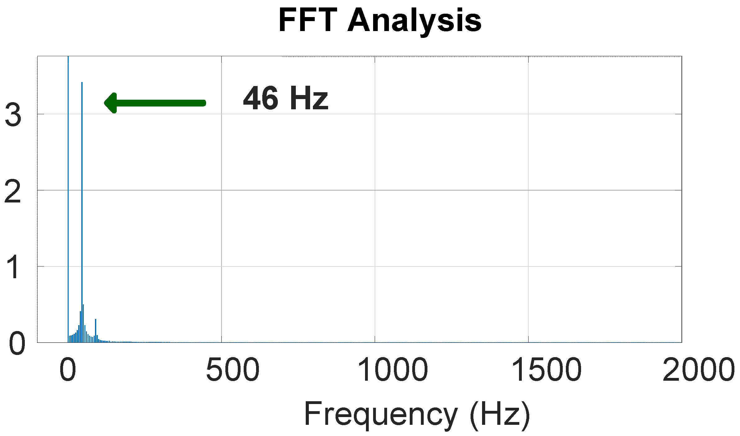
The SC plays a crucial role in mitigating SSOs in the HVAC CIGRE Benchmark model. To simulate a critical weak grid scenario with dynamic instability, the short-circuit ratio (SCR) of the model is reduced to a critical value of instability, equal to , as defined in [27].
This leads to an increase in array cable impedance, creating a critical case where SSOs occur and the system becomes unstable. However, the connection of the SC mitigates these SSOs, with the effectiveness of mitigation depending on the rating of the SC, as shown in Figure 20. The oscillation frequency of the SSOs is shown in Figure 21.
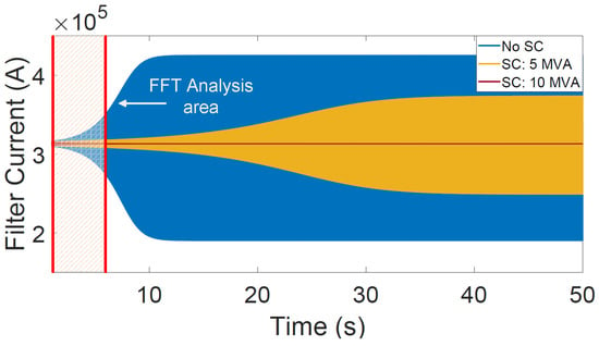
Figure 20.
Filter current of the grid-following converter system in the HVAC CIGRE benchmark model with SC when under three different cases of low SC power ratings (0, 5, and 10 MVA).
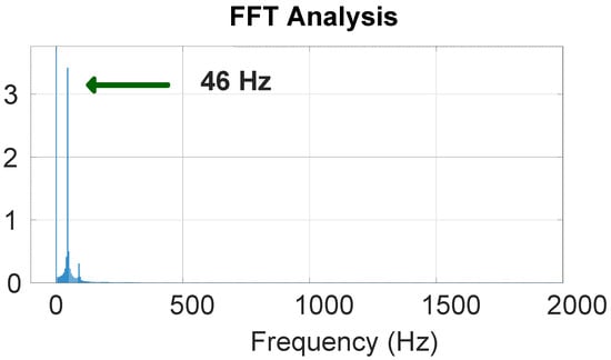
Figure 21.
FFT analysis of the filter current in the HVAC CIGRE benchmark model when and SSOs are not mitigated.
The EMT simulation in Figure 20 demonstrates that a higher rating of the SC machine results in normal and stable operation. Specifically, when the SC’s rating is 5 MVA, SSOs are not mitigated but they are mitigated when the rating is increased to 10 MVA. It has been observed that a rating of approximately 10 MVA is the lowest acceptable boundary for SC ratings.
However, it is important to consider the capacity of the wind farm, which is 240 MW, when connecting an SC to it. Time domain simulations in this paper have shown that if an SC with a very high rating is connected to the onshore substation of the wind farm, it may bring the system to normal operation quickly but may also result in the emergence of SSOs.
In fact, Figure 22 shows that there are no any oscillations when the SC rating is equal to 90 MVA. However, in case the rating of SCs is set to 110 MVA, subsynchronous oscillations arise at s and the corresponding EMT simulations are shown in the same figure. In addition, if the SC rating is increased to 150 MVA, the system becomes unstable much faster, at approximately 22 s. Therefore, the SSOs associated with the relatively high rating of the incorporated SC into the wind farm are not pre-existing oscillations. Instead, these oscillations emerge due to the high power rating of the SC, which necessitates the need to set an upper limit on it.
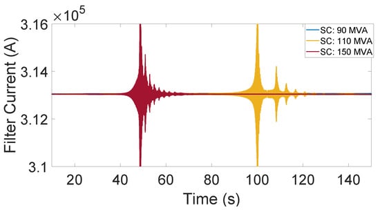
Figure 22.
Filter current of the grid-following converter system in the HVAC CIGRE benchmark model with SC when under three different cases of high SC power ratings (90, 110, and 150 MVA).
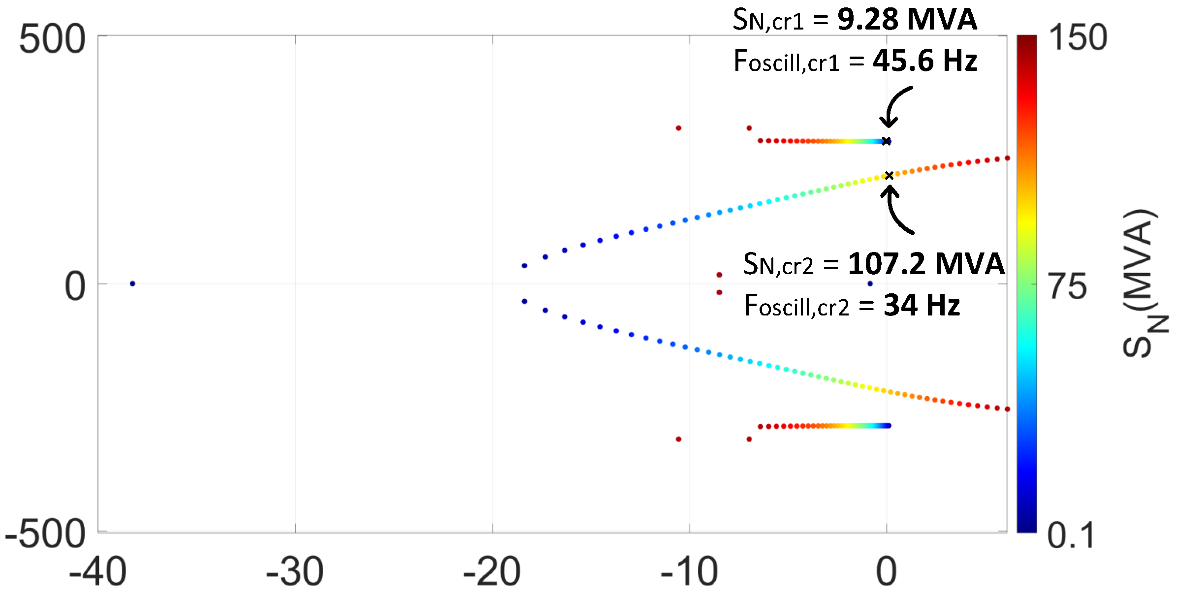
The small-signal model of the HVAC CIGRE Benchmark model with the SC is then examined. Eigenvalue-based stability analysis is implemented and the eigenvalue trajectory is observed in Figure 23, while the SC’s power rating is varied.
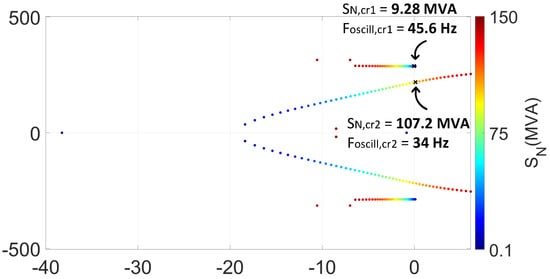
Figure 23.
Eigenvalue-based stability analysis of the small-signal model corresponding to the HVAC CIGRE benchmark model with the SC. The trajectories for SC’s rating are shown.
Based on the eigenvalue trajectory, it is noticed that when , the system is initially unstable with an oscillation frequency of Hz. When an SC with a rating of 9.28 MVA is connected, the system becomes stable. Nevertheless, when the rating of the SC is increased to 107.2 MVA, another mode becomes unstable with an oscillatory frequency of Hz. This indicates that there is a range of acceptable SC ratings in the MVA range for the critical case of in the wind farm system under study.
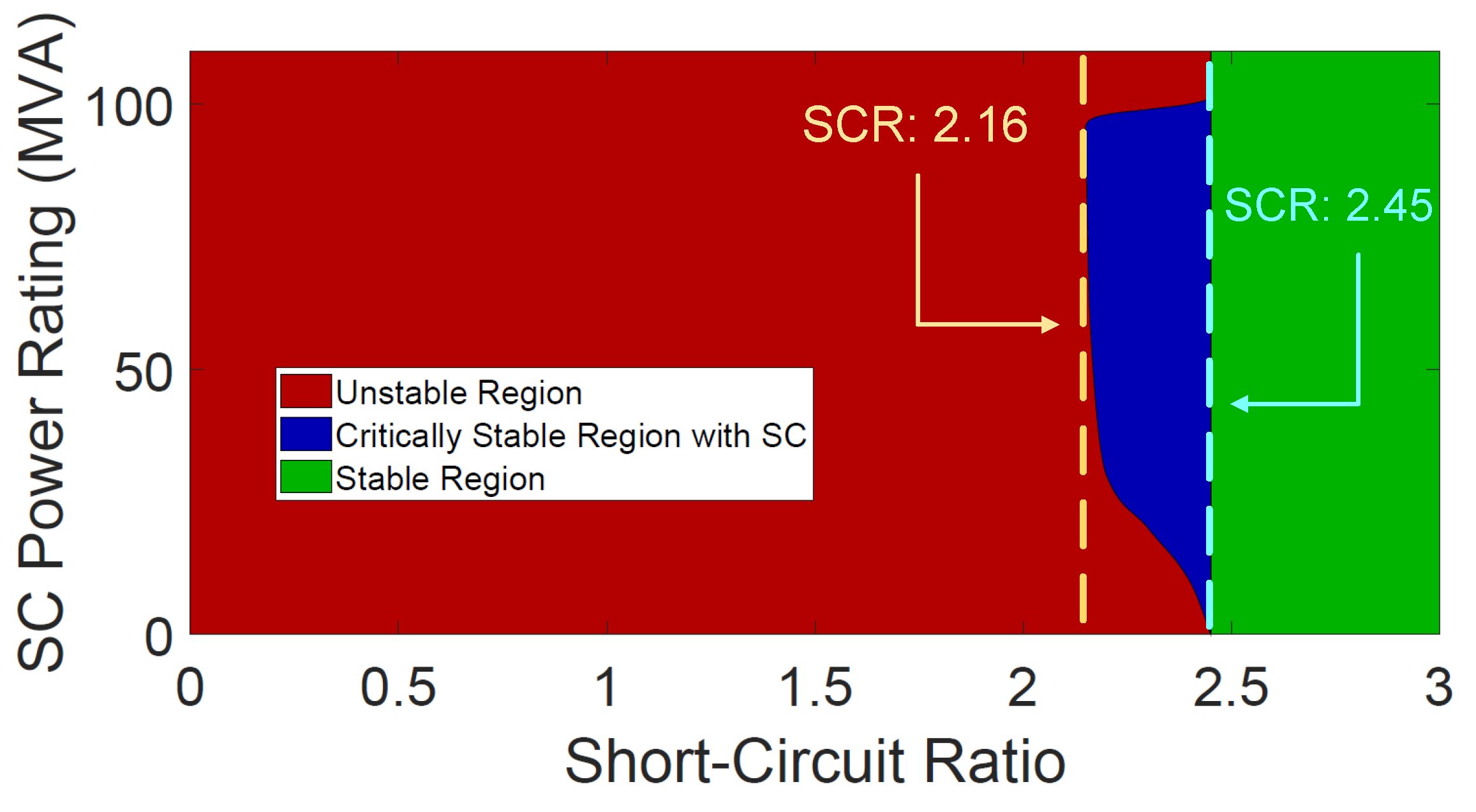
This finding is consistent with the EMT simulation results shown in Figure 20 and Figure 22, demonstrating a high level of accuracy of the small-signal model in selecting an optimal SC for mitigating SSOs in a specific critical case of a weak grid. The acceptable range of SCs’ power rating could be visualized for all possible SCR cases around the critical case of and it is shown in Figure 24.

Figure 24.
Acceptable SCs’ power ratins for all possible SCRs corresponding to a weak grid in the wind farm under study (240 MW). Green region is stable. Blue region can be stabilized with an SC. Red region is unstable and cannot be stabilized.
Therefore, depending on the wind farm model under study and also considering unchanged AVR parameters, the small-signal model under study can be proven to be of valuable importance for selecting the optimal SC in order to mitigate SSOs successfully and ensure the system’s stability.
5. Conclusions
This paper has examined the small-signal stability impact of an SC’s power rating on wind farms. For this purpose, a small-signal model for wind farms is utilized, considering an aggregated grid-connected converter that adopts the grid-following control and the passive elements, which consist of cables and transformers for the connection to the grid. This model, which is based on the HVAC CIGRE benchmark model, incorporates the validated state-space submodel of the SC in order to examine the stability impact of its power rating during weak grid conditions. The implementation of the SC, with a minimum rating of 10 MVA, effectively attenuates the SSOs observed in weak-grid scenarios. However, in case the AVR’s parameters in the SC remain unchanged, the eigenvalue-based stability analysis determines a maximum acceptable SC rating to be approximately half of the wind farm’s capacity in order to avoid the resurgence of instability issues. Considering the wind farm model under study, when it is rated at 240 MW, the maximum acceptable SC rating is determined to be 107.2 MVA. This research further substantiates its findings through time-domain simulations and FFT analysis, confirming the validity of the outcomes. The developed model and the findings give a novel method for doing an optimal selection of a synchronous condenser in addressing SSOs. Future investigations may explore the impact of other SC characteristics as well as other control structures in the wind farms.
Author Contributions
Conceptualization, D.D., M.K.B., L.K., X.W. and F.B.; methodology, D.D.; software, D.D.; validation, D.D.; formal analysis, D.D.; investigation, D.D., M.K.B., L.K., X.W. and F.B.; resources, M.K.B., L.K., X.W. and F.B.; data curation, D.D.; writing—original draft preparation, D.D.; writing—review and editing, D.D., M.K.B., L.K., X.W. and F.B.; visualization, D.D.; supervision, M.K.B., L.K., X.W. and F.B.; project administration, D.D.; funding acquisition, X.W. and F.B. All authors have read and agreed to the published version of the manuscript.
Funding
This project received funding from the European Union’s Horizon 2020 research and innovation program under the Marie Sklodowska-Curie grant agreement no. 861398.
Data Availability Statement
The original contributions presented in the study are included in the article, further inquiries can be directed to the corresponding author.
Conflicts of Interest
Authors Mohammad Kazem Bakhshizadeh and Lukasz Kocewiak were employed by Ørsted Wind Power A/S. The remaining authors declare that the research was conducted in the absence of any commercial or financial relationships that could be construed as a potential conflict of interest.
Appendix A
The wind turbine parameters are obtained from the HVAC CIGRE benchmark model [6]. For simplicity, the mechanical system of the wind turbines is not considered in this analysis. The system and control parameters of the grid-connected converter, as well as the parameters of the transformers and cables, are given in Table A1, Table A2, Table A3 and Table A4.
Table A1.
System parameters of the converter system.
Table A1.
System parameters of the converter system.
| Description | Value | |
|---|---|---|
| fsw | Switching Frequency | 2950 Hz |
| fS | Sampling Frequency | 5900 Hz |
| Sb | Rated Power | 12 MW |
| Vb | L-L RMS Voltage | 690 V |
| LF | Filter Inductance | 0.1056 pu |
| RF | Filter Resistance | 0.0053 pu |
| CF | Filter Capacitance | 0.0757 pu |
| LS | Output Inductance | 0.0261 pu |
| RS | Output Resistance | 0.0054 pu |
Table A2.
Control parameters of the converter system.
Table A2.
Control parameters of the converter system.
| Description | Value | |
|---|---|---|
| KI,CC0 | Default Integral Gain of Current Control | 0.1246 |
| KP,CC0 | Default Proportional Gain of Current Control | 0.0004 |
| KD | Active Damping Gain of Current Control | 0.0004 |
| KFFV | Feedforward Gain of Current Control | 1 |
| KI,PLL0 | Default Integral Gain of PLL | 0.9106 |
| KP,PLL0 | Default Proportional Gain of PLL | 0.0455 |
Table A3.
Transformer parameters.
Table A3.
Transformer parameters.
| Grid Transformer | |
| Description | Value |
| Voltage Ratio (kV/kV) | 400/220 |
| Rated Power (MVA) | 430 |
| Inductance (H) | 0.12 |
| Resistance () | 0.0014 |
| Power Plant Transformer | |
| Description | Value |
| Voltage Ratio (kV/kV) | 220/66 |
| Rated Power (MVA) | 270 |
| Inductance (H) | 0.12 |
| Resistance () | 0.0025 |
| PGU Transformer | |
| Description | Value |
| Voltage Ratio (kV/kV) | 66/0.69 |
| Rated Power (MVA) | 240 |
| Inductance (H) | 0.0261 |
| Resistance () | 0.0054 |
| Synchronous Condenser Transformer | |
| Description | Value |
| Voltage Ratio (kV/kV) | 26/220 |
| Rated Power (MVA) | 270 |
| Inductance (H) | 0.14 |
| Resistance () | 20 |
Table A4.
Cable parameters.
Table A4.
Cable parameters.
| 500 mm2 Array Cable 66 kV | |
|---|---|
| Description | Value |
| Inductance | 0.34 mH/km |
| Resistance | 0.06 /km |
| Capacitance | 0.29 F/(km/2) |
| 150 mm2 Array Cable 66 kV | |
| Description | Value |
| Inductance | 0.14 mH/km |
| Resistance | 0.41 /km |
| Capacitance | 0.19 F/(km/2) |
| HVAC Cable 220 kV | |
| Description | Value |
| Inductance | 0.406 mH/km |
| Resistance | 0.047 /km |
| Capacitance | 0.208 F/(km/2) |
Appendix B
The parameters of the synchronous condenser included in the HVAC CIGRE benchmark model—synchronous generator and AVR parameters—are shown in Table A5.
Table A5.
Parameters of the synchronous generator and automatic voltage regulator (AVR) in a synchronous condenser. The rating depends on the case under study.
Table A5.
Parameters of the synchronous generator and automatic voltage regulator (AVR) in a synchronous condenser. The rating depends on the case under study.
| Description | Value | |
|---|---|---|
| Rated Power | - | |
| Base Voltage | 26 kV | |
| Base Frequency | 50 Hz | |
| Mutual air-gap inductance d-axis | 2.1 pu | |
| Mutual air-gap inductance q-axis | 2.1 pu | |
| Leakage inductance in stator winding | 0.35 pu | |
| Leakage inductance in field winding | 0.22 pu | |
| Leakage inductance in damper winding d-axis | 0.1826 pu | |
| Leakage inductance in damper winding q-axis | 0.1281 pu | |
| D | Damping Constant | 1 pu |
| Armature Resistance | 0.007 pu | |
| Field Winding Resistance | 0.0016 pu | |
| Damper Winding Resistance d-axis | 0.0085 pu | |
| Damper Winding Resistance q-axis | 0.0085 pu | |
| H | Inertia | 4 s |
| Exciter Gain | 5 pu | |
| Exciter Time Constant | 0.0065 s | |
| Transducer Time Constant | 0.001 s |
The relations between the inductances of the synchronous generator are described in Table A6.
Table A6.
Synchronous generator’s inductances relations.
Table A6.
Synchronous generator’s inductances relations.
| Inductance | Description |
|---|---|
| Ld = Lad + Lal | Self inductance of d-axis stator winding |
| Lq = Laq + Lal | Self inductance of q-axis stator winding |
| Lffd = Lad + Lfdl | Self inductance in field winding d-axis |
| Lkkd = Lad + Lkdl | Self inductance in damper winding d-axis |
| Lkkq = Lad + Lkql | Self inductance in damper winding q-axis |
References
- Bada, J.; Vidal, A.D.; Komazawa, Y.; Ledanois, N.; Yaqoob, H.; Brown, A.; Sawin, J.L.; Abdelnabi, H.; Couzin, H.; El Guindy, A.; et al. Renewables 2023 Global Status Report; Report REN21.2023; REN21 Secretariat: Paris, France, 2023. [Google Scholar]
- IRENA. Renewable Capacity Statistics 2023; International Renewable Energy Agency: Abu Dhabi, United Arab Emirates, 2023. [Google Scholar]
- Global Wind Energy Council. Global Wind Report 2023; Global Wind Energy Council: Belgium, Brussels, 2023. [Google Scholar]
- Wang, X.; Blaabjerg, F. Harmonic Stability in Power Electronic-Based Power Systems: Concept, Modeling, and Analysis. IEEE Trans. Smart Grid 2019, 10, 2858–2870. [Google Scholar] [CrossRef]
- Flynn, D.; Rather, Z.; Årdal, A.R.; D’Arco, S.; Hansen, A.D.; Cutululis, N.A.; Sorensen, P.; Estanqueiro, A.; Gómez-Lázaro, E.; Menemenlis, N.; et al. Technical impacts of high penetration levels of wind power on power system stability. WIREs Energy Environ. 2017, 6, e216. [Google Scholar] [CrossRef]
- Kocewiak, L.; Blasco-Giménez, R.; Buchhagen, C.; Kwon, J.B.; Sun, Y.; Trevisan, A.S.; Larsson, M.; Wang, X. Overview, status, and outline of stability analysis in converter-based power systems. In Proceedings of the 19th International Wind Integration Workshop, Virtual, 11–12 November 2020; p. 10. [Google Scholar]
- Gu, K.; Wu, F.; Zhang, X. Sub-synchronous interactions in power systems with wind turbines: A review. IET Renew. Power Gener. 2019, 13, 4–15. [Google Scholar] [CrossRef]
- Cheng, Y.; Fan, L.; Rose, J.; Huang, S.H.; Schmall, J.; Wang, X.; Xie, X.; Shair, J.; Ramamurthy, J.R.; Modi, N.; et al. Real-World Subsynchronous Oscillation Events in Power Grids With High Penetrations of Inverter-Based Resources. IEEE Trans. Power Syst. 2023, 38, 316–330. [Google Scholar] [CrossRef]
- Zhou, G.; Wang, D.; Atallah, A.; McElvain, F.; Nath, R.; Jontry, J.; Bolton, C.; Lin, H.; Haselbauer, A. Synchronous condenser applications: Under significant resource portfolio changes. IEEE Power Energy Mag. 2019, 17, 35–46. [Google Scholar] [CrossRef]
- Nguyen, H.T.; Yang, G.; Nielsen, A.H.; Jensen, P.H. Combination of Synchronous Condenser and Synthetic Inertia for Frequency Stability Enhancement in Low-Inertia Systems. IEEE Trans. Sustain. Energy 2019, 10, 997–1005. [Google Scholar] [CrossRef]
- Hadavi, S.; Mansour, M.Z.; Bahrani, B. Optimal allocation and sizing of synchronous condensers in weak grids with increased penetration of wind and solar farms. IEEE Trans. Emerg. Sel. Topics Circuits Syst. 2021, 11, 199–209. [Google Scholar] [CrossRef]
- Wang, Y.; Wang, L.; Jiang, Q. Impact of synchronous condenser on sub/super-synchronous oscillations in wind farms. IEEE Trans. Power Del. 2021, 36, 2075–2084. [Google Scholar] [CrossRef]
- Ganjefar, S.; Farahani, M. Comparing SVC and synchronous condenser performance in mitigating torsional oscillations. Int. Trans. Electr. Energy Syst. 2015, 25, 2819–2830. [Google Scholar] [CrossRef]
- Bao, L.; Fan, L.; Miao, Z. Comparison of Synchronous Condenser and STATCOM for Wind Farms in Weak Grids. In Proceedings of the 2020 52nd North American Power Symposium (NAPS), Tempe, AZ, USA, 11–13 April 2021; pp. 1–6. [Google Scholar]
- Jia, J.; Yang, G.; Nielsen, A.H.; Gevorgian, V. Investigation on the Combined Effect of VSC-Based Sources and Synchronous Condensers Under Grid Unbalanced Faults. IEEE Trans. Power Deliv. 2019, 34, 1898–1908. [Google Scholar] [CrossRef]
- Jia, J.; Yang, G.; Nielsen, A.H.; Rønne-Hansen, P. Impact of VSC Control Strategies and Incorporation of Synchronous Condensers on Distance Protection Under Unbalanced Faults. IEEE Trans. Ind. Electron. 2019, 66, 1108–1118. [Google Scholar] [CrossRef]
- Richard, L.; Nahid-Al-Masood; Saha, T.K.; Tushar, W.; Gu, H. Optimal Allocation of Synchronous Condensers in Wind Dominated Power Grids. IEEE Access 2020, 8, 45400–45410. [Google Scholar] [CrossRef]
- Jia, J.; Yang, G.; Nielsen, A.H.; Muljadi, E.; Weinreich-Jensen, P.; Gevorgian, V. Synchronous Condenser Allocation for Improving System Short Circuit Ratio. In Proceedings of the 2018 5th International Conference on Electric Power and Energy Conversion Systems (EPECS), Kitakyushu, Japan, 23–25 April 2018; pp. 1–5. [Google Scholar]
- Hadavi, S.; Saunderson, J.; Mehrizi-Sani, A.; Bahrani, B. A Planning Method for Synchronous Condensers in Weak Grids Using Semi-Definite Optimization. IEEE Trans. Power Syst. 2023, 38, 1632–1641. [Google Scholar] [CrossRef]
- Arraño-Vargas, F.; Shen, Z.; Jiang, S.; Fletcher, J.; Konstantinou, G. Challenges and mitigation measures in power systems with high share of renewables—The Australian experience. Energies 2022, 15, 429. [Google Scholar] [CrossRef]
- Amin, M.; Molinas, M. Small-Signal Stability Assessment of Power Electronics Based Power Systems: A Discussion of Impedance- and Eigenvalue-Based Methods. IEEE Trans. Ind. Appl. 2017, 53, 5014–5030. [Google Scholar] [CrossRef]
- Dimitropoulos, D.; Wang, X.; Blaabjerg, F. Small-Signal Stability Analysis of Grid-Connected Converter under Different Grid Strength Cases. In Proceedings of the 2022 IEEE 13th International Symposium on Power Electronics for Distributed Generation Systems (PEDG), Kiel, Germany, 26–29 June 2022; pp. 1–6. [Google Scholar]
- Dimitropoulos, D.; Wang, X.; Blaabjerg, F. Stability Impacts of an Alternate Voltage Controller (AVC) on Wind Turbines with Different Grid Strengths. Energies 2023, 16, 1440. [Google Scholar] [CrossRef]
- Dowlatabadi, M.B. Harmonic Modelling, Propagation and Mitigation for Large Wind Power Plants Connected via Extra Long HVAC Cables: With Special Focus on Harmonic Stability. Ph.D. Thesis, Aalborg Universitetsforlag, Aalborg, Denmark, 2018. [Google Scholar]
- Kanálik, M.; Margitová, A.; Kolcun, M. Modeling of synchronous machines including voltage regulation. Prz. Elektrotechniczny 2019, 95, 125–132. [Google Scholar] [CrossRef]
- Anderson, P.M.; Agrawal, B.L.; Ness, J.E.V. Subsynchronous Resonance in Power Systems; IEEE Press: New York, NY, USA, 1990. [Google Scholar]
- CIGRE. Connection of Wind Farms to Weak AC Networks; W. G. B4.62; CIGRE Technical Brochure; CIGRE: Paris, France, 2016. [Google Scholar]


Disclaimer/Publisher’s Note: The statements, opinions and data contained in all publications are solely those of the individual author(s) and contributor(s) and not of MDPI and/or the editor(s). MDPI and/or the editor(s) disclaim responsibility for any injury to people or property resulting from any ideas, methods, instructions or products referred to in the content. |
© 2024 by the authors. Licensee MDPI, Basel, Switzerland. This article is an open access article distributed under the terms and conditions of the Creative Commons Attribution (CC BY) license (https://creativecommons.org/licenses/by/4.0/).