Possibilities of Utilising Biomass Collected from Road Verges to Produce Biogas and Biodiesel

Czubaszek, Robert; Wysocka-Czubaszek, Agnieszka; Sienkiewicz, Aneta; Piotrowska-Niczyporuk, Alicja; Wassen, Martin J.; Bajguz, Andrzej

doi:10.3390/en17071751

Open AccessArticle

Possibilities of Utilising Biomass Collected from Road Verges to Produce Biogas and Biodiesel

¹

Faculty of Civil Engineering and Environmental Sciences, Bialystok University of Technology, Wiejska 45A Street, 15-351 Bialystok, Poland

²

Department of Biology and Plant Ecology, Faculty of Biology, University of Bialystok, Ciolkowskiego 1J Street, 15-245 Bialystok, Poland

³

Copernicus Institute of Sustainable Development, Faculty of Geosciences, Utrecht University, Princetonlaan 8a, 3584 CB Utrecht, The Netherlands

^*

Author to whom correspondence should be addressed.

Energies 2024, 17(7), 1751; https://doi.org/10.3390/en17071751

Submission received: 16 March 2024 / Revised: 30 March 2024 / Accepted: 3 April 2024 / Published: 5 April 2024

(This article belongs to the Special Issue Sustainable Energy Development in Liquid Waste and Biomass)

Download

Browse Figures

Versions Notes

Abstract

:

Grass collected as part of roadside maintenance is conventionally subjected to composting, which has the disadvantage of generating significant CO₂ emissions. Thus, it is crucial to find an alternative method for the utilisation of grass waste. The aim of this study was to determine the specific biogas yield (SBY) from the anaerobic mono-digestion of grass from road verges and to assess the content of Fatty Acid Methyl Esters (FAMEs) in grass in relation to the time of cutting and the preservation method of the studied material. The biochemical biogas potential (BBP) test and the FAMEs content were performed on fresh and ensiled grass collected in spring, summer, and autumn. The highest biogas production was obtained from fresh grass cut in spring (715.05 ± 26.43 NL kg_VS⁻¹), while the minimum SBY was observed for fresh grass cut in summer (540.19 ± 24.32 NL kg_VS⁻¹). The methane (CH₄) content in the biogas ranged between 55.0 ± 2.0% and 60.0 ± 1.0%. The contents of ammonia (NH₃) and hydrogen sulphide (H₂S) in biogas remained below the threshold values for these inhibitors. The highest level of total FAMEs was determined in fresh grass cut in autumn (98.08 ± 19.25 mg g_DM⁻¹), while the lowest level was detected in fresh grass cut in spring (56.37 ± 7.03 mg g_DM⁻¹). C16:0 and C18:0, which are ideal for biofuel production, were present in the largest amount (66.87 ± 15.56 mg g_DM⁻¹) in fresh grass cut in autumn. The ensiling process significantly impacted the content of total FAMEs in spring grass, leading to a reduction in total saturated fatty acids (SFAs) and an increase in total unsaturated fatty acids (USFAs). We conclude that grass biomass collected during the maintenance of road verges is a valuable feedstock for the production of both liquid and gaseous biofuels; however, generating energy from biogas appears to be more efficient than producing biodiesel.

Keywords:

biogas; grass; road verges; FAME

1. Introduction

Economic growth, a population that has doubled since 1970, and accelerated material extraction, coupled with an increase in waste, have led to substantial transformations in land use and forest cover. These factors have also induced land degradation, climate change, biodiversity decrease, eutrophication, and pollution of waterways and soils [1]. Cities, which are responsible for generating 80% of the global domestic product [2], are currently undergoing rapid economic growth, resulting in increased rural-to-urban migration [3]. Presently, 55% of the world’s population resides in urban areas [4], while in Europe, nearly 75% of the population lives in cities [5]. Many cities grapple with problems such as inadequate infrastructure, traffic congestion [3], energy-inefficient building stock, and air pollution. Nonetheless, in the forthcoming decades, urban areas are expected to be the most profoundly affected by climate change [5]. Conversely, cities are significant contributors to climate change, emitting 71–76% of global anthropogenic carbon dioxide (CO₂). The realisation of the 11th Sustainable Development Goal (Sustainable Cities and Communities) from Resolution 70/1, adopted by the UN General Assembly on 25 September 2015, titled “Transforming our world: the 2030 Agenda for Sustainable Development”, necessitates intelligent urban planning aimed at creating resilient cities [6]. In the European Union (EU), the European Green Deal set a target to transform Europe into a climate-neutral continent by 2050 through a reduction in greenhouse gas (GHG) emissions of at least 55%, compared to 1990 levels. Achieving this goal requires, among other measures, an increase in the share of energy from renewable sources in the EU’s energy mix to 40% [7]. The European urban landscape is characterised by small and medium-sized cities, which are expected to play a pivotal role in the development of a sustainable and climate-neutral Europe [5].

Urban green areas, as defined by the Nature Conservation Act of April 2004 [8], encompass areas with technical infrastructure and buildings functionally linked to them, covered with vegetation and serving public functions, particularly including parks; promenades; boulevards; botanical, zoological, and historical gardens; and cemeteries. Urban green areas also include greenery along roads in built-up areas, squares, historic fortifications, buildings, landfills, airports, railway stations, and industrial facilities. Urban green areas are situated within the administrative borders of cities, providing aesthetic, recreational, and health functions [9]. Green areas in urban landscapes enhance air quality, mitigate extreme weather events, and regulate the hydrological cycle [10,11]. Additionally, green spaces in cities effectively alleviate the urban heat island effect [12,13] and play a crucial role in city resilience [14]. Consequently, urban systems with extensive green infrastructure exhibit greater resilience to crises and are more human-friendly [15]. The maintenance of urban green areas is indispensable for their diverse roles in cities, encompassing aesthetic aspects, environmental benefits, stormwater management, urban heat island mitigation, and community cohesion. Maintenance tasks in urban green spaces include trimming, irrigation, fertilisation, and pesticide application [16]. Mowing grass on road verges is conducted to maintain visibility and safety. The cut grass is either left to decay or collected and utilised. However, the maintenance of green areas involves significant labour and machine input, consuming energy resources and resulting in waste generation. Trimming, fertilising, and waste transport consume fossil fuels and emit GHGs into the atmosphere [17]. Despite recent reductions in maintenance workload through improved working plans, decreased trimming frequency, the introduction of wildflowers and meadows, and the self-maintenance of green spaces, large areas, such as sports fields and road verges, are still frequently trimmed. In addition, the policy of urban greenery extension results in increase in both the workload associated with its maintenance and with the amount of biomass produced, which needs to be utilised in a sustainable way [17].

The biobased and circular economy, considered a viable approach for sustainable development, directs societies toward the sequential utilisation of resources, with an emphasis on biomass and bio-waste. The diminishing availability of resources, coupled with an escalating demand for energy and food, underscores the need to optimize the efficient use of biomass and bio-waste. Grass-trimming biomass is commonly subjected to composting, an aerobic process that transforms lignocellulosic waste into a value-added product, namely compost. However, this process is associated with substantial GHG emissions. Furthermore, the utilisation of immature compost may result in water pollution, odour emissions, and adverse effects on plant germination and development [18]. As an alternative, other methods of bio-waste utilisation, such as biogas production, are being explored. The utilisation of green waste for energy generation has the potential to mitigate the elevated fuel consumption and GHG emissions associated with maintaining expanded green spaces within urban areas.

The anaerobic digestion (AD) of grass offers benefits, including waste reduction, decreased GHG emissions, and the generation of renewable energy and valuable fertilizer. However, the biogas potential of grass is relatively low, particularly when compared to biogas production from maize [19]. The specific methane yield (SMY) has been extensively studied across various wild and cultivated grass species [20,21,22,23,24,25,26]. Additionally, co-digestion of grass and other substrates as a strategy to enhance biogas production has been investigated [27,28]. The harvesting date is a critical factor affecting grass SMY, as the lignification process intensifies with advancing maturity, limiting material digestibility [29]. Dragoni et al. [24] noted higher SMY from AD of leaves compared to stems due to their elevated protein content [20].

Another possibility for utilising waste generated during road verges maintenance involves the production of biodiesel. Biodiesel, primarily comprising Fatty Acid Methyl Esters (FAMEs), can be derived from various waste biomasses, including olive pomace oil [30], cooking palm oil [31], beef tallow [32], fish fat [33], chicken fat [34], citrus wax [35], and sewage sludge [36]. Additionally, biodiesel production from spent coffee grounds [37], cherry stone waste [38], and herbal waste [39] represents another feasible approach to resource utilisation. This not only aids in reducing crude oil consumption but also contributes to mitigating GHG emissions and air pollution.

The aim of this study was to determine the potential to obtain material from grass from road verges for the production of liquid biofuels (biodiesel) and to determine the specific biogas yield (SBY) from anaerobic mono-digestion of the studied grass in relation to the time of cutting and the preservation method of the studied material. Since a continuous supply of feedstock is essential for biofuel production, the study was conducted on both fresh and ensiled grass.

2. Materials and Methods

2.1. Substrates and Inoculum

The biogas potential and FAME content were assessed using grass samples harvested from the city of Białystok (53°07’ N, 23°09’ E, 136 m a.s.l.) in the northeastern region of Poland. Białystok, serves as the capital city of the Podlaskie voivodeship, covering an area of 102 km², and has a population of 292,000 citizens [40]. The climatic conditions are characterised by an average annual temperature of 7.4 °C and an average annual precipitation of 590 mm, predominantly occurring from May to August [41]. The species composition of the grassed verges was predominantly composed of perennial ryegrass (Lolium perenne L.), accompanied by Kentucky bluegrass (Poa pratensis L.) and red fescue (Festuca rubra L.). Plant material was collected on three occasions in the year 2019: in spring (25 April), summer (31 July), and autumn (7 October). During each collection, the grass was acquired from piles of mown material along the streets, as part of the green area maintenance conducted by an external company employed by the City Hall of Białystok. Following collection, the plant material was promptly transported to the laboratory and homogenised. The moisture content of the fresh material was determined by subjecting it to drying at 105 ± 2 °C until a constant weight was achieved. The material designated for ensiling was allowed to air-dry at room temperature for 24 h. Subsequently, it was cut into lengths of 2–4 cm and ensiled without the addition of any additives for 5–6 weeks. After this period, the moisture content was determined. The chemical composition of both fresh grass and silage is presented in Table 1.

The inoculum for all three biochemical biogas potential (BBP) tests comprised digestate obtained from a mesophilic agricultural biogas plant which was supplied with maize silage supplemented with 10–20% food and agricultural wastes. Prior to the BBP test, the digestate was degassed at a temperature of 38 °C. The chemical properties of the inocula used in all three experiments are presented in Table 2.

2.2. Biochemical Biogas Potential Tests

The BBP test was conducted using wet technology in OxiTop^® reactors (WTW, Weilheim, Germany) with a volume of 1 L and a working volume of approximately 300 mL. The reactors were incubated in a thermostatic incubator at 38 ± 1 °C. The substrates and inoculum were added to the reactors in a ratio of 2:1 VS_inoculum to VS_substrate. To maintain anaerobic conditions, the reactors were subjected to a 2 min flush with nitrogen. The BBP tests were performed in triplicate, along with three control reactors filled solely with inoculum and water. Biogas production was monitored at intervals of 240 min based on pressure changes within the reactor, facilitated by the OxiTop® measuring head. The composition of the biogas was analysed using the portable biogas analyzer DP-28BIO (Nanosens, Wysogotowo, Poland) from samples taken with 20 mL gas-tight glass syringes. Biogas composition assessments were conducted daily initially, transitioning to twice a week after the experiment had run for 10 days.

2.3. Transesterification Procedure

Grass samples (1 g) underwent extraction with hexane in the presence of a methanol-potassium hydroxide (KOH) mixture acting as a catalyst with the synthesis process involving the addition of hexane. An analysis using gas chromatography–mass spectrometry in the selected ion monitoring mode (GC-MS/SIM) quantified the presence of up to 31 FAMEs in the grass samples (Table 3). A comprehensive description of the transesterification procedure, i.e., the optimal extraction conditions, is presented in the study by Sienkiewicz et al. [39].

2.4. Calculations and Statistical Analyses

The BBP test was conducted until the daily biogas production accounted for less than 1% of the total cumulative biogas volume observed over three consecutive days. SBY was calculated in units of NL kg_VS⁻¹ (NL = normal litre, i.e., gas volume corrected to 0 °C and 1.013 bar). The kinetics of biogas production were determined using the modified Gompertz model [42]:

G (t) = G_{0} \times e x p \{- e x p [\frac{R_{m a x} \times e}{G_{0}} (λ - t) + 1]\}

(1)

where

G(t)—cumulative biogas production at a specific time t (mL);
G₀—biogas production potential (mL);
R_max—maximum daily biogas production rate (mL day⁻¹);
λ—duration of lag phase (minimum time to produce biogas) (days);
t—cumulative time taken to achieve biogas production (days);
e—mathematical constant (2.71828).

In addition, based on the plotted curves, the time (days) when 50% (T50) and 95% (T95) of the possible biogas production were reached was determined.

For the calculations of the amount of energy contained in liquid biofuel obtained from grass, the heating value of methyl esters of fatty acids was adopted at 37 MJ kg⁻¹ [43]. For the calculations of the avoided carbon dioxide emissions by replacing coal with biogas, emission values of 93.54 kg CO₂ GJ⁻¹ [44] and 685 kg CO₂ MWh⁻¹ [45] were adopted, respectively, for thermal and electric energy production. In the case of using biodiesel as a substitute for fossil fuel, the diesel oil emission of 74.1 kg CO₂ GJ⁻¹ [44] was adopted.

Significant differences in cumulative biogas production, as well as methane (CH₄), hydrogen sulphide (H₂S), and ammonia (NH₃) concentrations in biogas from fresh and ensiled grasses cut in spring, summer, and autumn were assessed with a two-way analysis of variance (ANOVA), using the method of grass preservation and the cutting time as fixed factors. Significant differences in FAMEs between the cutting time of fresh grass and ensiled grass were assessed with a one-way analysis of variance. Differences between means were determined using Tukey’s Honest Significant Difference (HSD) test. The homogeneity of variance and normality were checked prior to ANOVA using the Levene and Shapiro–Wilk tests, respectively. Principal Component Analysis (PCA) was performed to build the relationship model between variables. The first seventeen factors were preserved in a biplot for further analysis. The final biplot was created using the two main components (PC1 and PC2), which together explain 61.8% of the total variance. The level of accepted statistical significance was set at p < 0.05. All statistical analyses of the data were performed using STATISTICA 13.3 software (TIBCO Software Inc., Palo Alto, CA, USA).

3. Results

3.1. Biogas Production

The cutting time significantly influenced cumulative biogas production (p < 0.05). The highest biogas production was obtained from spring-cut grass, yielding 715.05 ± 26.43 NL kg_VS⁻¹ for fresh grass and 605.44 ± 6.19 NL kg_VS⁻¹ for grass silage. Conversely, the lowest biogas production was observed with fresh grass cut in summer (540.19 ± 24.32 NL kg_VS⁻¹) and grass silage from autumn (547.36 ± 1.20 NL kg_VS⁻¹). The ensiling process showed no effect on cumulative biogas production, except in the case of spring cutting, where biogas production from fresh grass exceeded that from ensiled grass (Figure 1).

The CH₄ content within the generated biogas, measured at the end of the experiment, displayed the highest values for spring-cut grass, whereas the lowest values were observed for autumn-cut grass (Table 4).

The preservation method did not exert any influence on the CH₄ concentration in the biogas. Nevertheless, the preservation method did impact the daily biogas production depending on the cutting time. In spring, the daily biogas production from FG-Sp exhibited higher values in the first 7 days, but subsequently experienced a significant decline by day 9. Concurrently, the daily biogas production from GS-Sp reached its peak on that day. The daily rates from both fresh and ensiled grasses became nearly identical on day 10, gradually decreasing to approximately 5 NL kg_VS⁻¹. In summer, daily biogas production from FG-Su increased rapidly in the first two days, followed by a decline on days 3 and 4, falling notably below the daily rate of biogas production from GS-Su. Subsequently, daily biogas production from FG-Su increased to the same value as daily biogas production from GS-Su and remained similar until the end of the experiment. In autumn, daily biogas production from both fresh and ensiled grasses displayed remarkable similarity to that observed at the beginning of the experiment. A swift increase occurred in the first 2 days, followed by a decrease from day 6 to day 8. After a brief period of heightened production, the daily rate declined and stabilised until the end of the experiment.

Notably, FG-Sp and FG-Au exhibited distinct behaviour compared to FG-Su. Daily biogas production from all three cutting times experienced rapid increases in the first 2 days. For FG-Sp and FG-Au, production remained elevated for the following 6 days. Conversely, daily biogas production from FG-Su, following an initial increase in the first 2 days, significantly decreased on days 3 and 4, dropping below the production from FG-Sp and FG-Au. Subsequently, the daily biogas production increased again, and the values for grasses from all three cutting times became similar. The daily biogas production from ensiled grass exhibited a consistent trend, irrespective of the cutting time (Figure 2). Regardless of the season and grass preservation method, significant biogas production persisted for approximately 14 days, displaying a dynamic course during this period.

Despite discernible fluctuations in the daily patterns of biogas production, the kinetics of biogas generation exhibited consistency across all cutting times and preservation methods. Regardless of the preservation technique employed and the timing of material cutting, the timeframe necessary for grass to achieve 50% of its potential biogas production (T50) varied between 5 and 6 days. The period required for grass to attain 95% of its potential biogas production ranged from 14 to 17 days (Figure 3).

3.2. Hydrogen Sulphide and Ammonia Concentration in Biogas

The inhibition of the AD process represents a significant impediment in the context of biogas production, wherein inhibitors may be introduced along with the feedstock or generated during distinct stages of process. Quantifying inhibitors, particularly NH₃ and H₂S levels in biogas, is crucial for influencing the conditions of biogas production. In this study, the NH₃ and H₂S contents remained at relatively low levels. Regardless of the cutting time, the H₂S content in the biogas exhibited higher values at the beginning of the experiment, subsequently demonstrating a significant decrease (p < 0.05) by the end of the experiment.

The initial H₂S content in biogas derived from spring-cut grass remained consistent at approximately 200 ppm, irrespective of the preservation method, and decreased to values around 100 ppm by the end of the experiment (Figure 4). Significantly higher values (p < 0.05) were observed in biogas from summer-cut grass, with an initial H₂S content of 749 ppm in biogas from FG-Su and 666 ppm in biogas from GS-Su. The final values for both fresh and ensiled grass were approximately 200 ppm. Although the highest initial H₂S content was observed in biogas from autumn-cut grass (exceeding 800 ppm), it was not significantly different from that of summer-cut grass. Notably, the final values aligned with those obtained from biogas derived from summer-cut grass. The ensiling process did not exert any significant effect on the H₂S concentration for any cutting time.

Biogas derived from spring-cut grass exhibited the lowest initial and final NH₃ concentrations, irrespective of the preservation method. Conversely, significantly higher values were observed in biogas from summer-cut grass (p < 0.05), with the highest NH₃ concentration found in biogas obtained from autumn-cut grass. In the case of biogas from FG-Sp and FG-Su, the disparities between initial and final NH₃ concentrations were not statistically significant. However, for grass silage, these differences were more pronounced. Biogas generated from autumn-cut grass displayed a notably elevated initial NH₃ concentration, which substantially decreased to approximately 100 ppm in the final stage of the experiment (Figure 5). The ensiling process did not affect the NH₃ concentration at any cutting time.

3.3. Identity and Composition of the Fatty Acid Methyl Esters

In both fresh and ensiled grass, up to 31 FAMEs were detected (Table 5, Table 6, Table 7 and Table 8). The total number of distinct fatty acid types ranged from 29 to 31. FG-Sp and FG-Su exhibited 29 fatty acid types, while GS-Au presented 31 types. In all the analysed grasses, irrespective of the preservation method and cutting time, nine monounsaturated fatty acids (MUFAs) were detected (Table 5). In FG-Sp and FG-Su, seven polyunsaturated fatty acids (PUFAs) (C18:2n6c, C18:3n6, C18:3n3, C20:3n6, C20:4n6, C22:2n6, and C22:6n3) were identified, whereas all eight PUFAs were detected in the remaining studied materials (Table 6). In fresh and ensiled grass cut during spring and summer, 13 saturated fatty acids (SFAs) were detected, while in GS-Au, 14 SFAs were found (Table 7).

The compositional analysis of the studied material revealed that the amount of SFA methyl esters (74.02–79.74%) exceeded that of unsaturated fatty acids (MUFAs and PUFAs) (Figure 6). The highest share of SFAs was identified in FG-Sp (79.74%), whereas the lowest SFA amount was observed in GS-Su (74.02%). The analysed grasses also exhibited distinct shares of MUFAs and PUFAs. The highest share of MUFAs was noted in GS-Sp (17%), while the lowest was observed in FG-Sp (13.4%). The highest share of PUFAs was noted in GS-Su (9.04%) and the lowest PUFAs were observed in FG-Sp (6.86%). The dominant FAMEs included C16:0 fatty acid, as well as C18:0, C18:1n9t/c, C18:2n6c, and C18:3n6 (Table 5, Table 6, Table 7 and Table 8), all of which are suitable for biofuel production. FG-Au exhibited the highest content of C16:0, C18:0, and C18:2n6c, while FG-Su had the highest concentrations of C18:1n9t/c and C18:3n6. Other FAMEs, such as C10:0, C11:0, C13:0, C14:1, C16:1, C17:1, C20:2, C20:3n6, C20:4n6, C21:0, C22:6n3, and C24:1n9, had a minimal impact on FAMEs composition, indicated by low content (i.e., less than about 100 µg g_DM⁻¹, Table 5, Table 6, Table 7 and Table 8).

The highest concentration of total FAMEs was determined in FG-Au and FG-Su (98.08 and 90.03 mg g_DM⁻¹, respectively, Table 8). C16:0 and C18:0 were found in the largest amounts (66.87 and 6.83 mg g_DM⁻¹, respectively) in FG-Au (Table 7). This is noteworthy, as these compounds are ideal for biofuel production. The lowest concentration of total FAMEs was detected in FG-Sp (56.37 mg g_DM⁻¹) and GS-Sp (58.42 mg g_DM⁻¹) (Table 8).

Principal Component Analysis facilitated the categorisation of the tested samples, maintaining a significant degree of explained variance. During this analysis, the variable count was condensed to two principal components (designated as PC1 and PC2), intimating that the initial dataset of 31 FAMEs is correlated and reducible (Figure 7). All variables, with the exception of C15:0, C22:6n3, and C24:1n9, presented positive loadings, ranging from 0.0479 (C14:1) to 0.9376 (C18:2n6c), in association with the first component. Contrastingly, C15:0 and C24:1n9 were associated with positive loadings (0.9232 and 0.0937, respectively), whereas C22:6n3 exhibited a negative loading (–0.1667) with the second component.

A comparison of case positions on the graph, considering component forms and factor loadings, revealed distinct characteristics among them. Specifically, Case 1, exhibiting positive coordinate values on the first axis, was identified as having a higher content of plant hormones, excluding C15:0, C22:6n3, and C24:1n9, according to the relevant factor loadings. Conversely, Case 2, with positive coordinate values for the second axis, was associated with higher C15:0, and C24:1n9 contents, based on the factor loadings with the second axis. In contrast, Case 3, showing a negative coordinate value on the second axis, was characterised by a lower C22:6n3 content, based on its factor loading with the second axis (Figure 7).

3.4. Energy Balance and CO₂ Reduction

In the assessment of the energy potential from the utilisation of grass from road verges, slightly higher quantities can be generated from fresh grass in comparison to grass silage (Table 9). This observed correlation is consistently reflected in the energy content of the liquid biofuel generated from the investigated grass. Notably, in the case of spring-cut grass, the energy content in biodiesel derived from ensiled grass slightly surpasses the value calculated for fresh grass. Comparing both examined biofuels produced from grass, it becomes evident that biogas production yields an approximately twofold increase in energy output.

A highly important aspect in favour of biofuel production is the mitigation of CO₂ emissions into the atmosphere generated during the combustion of fossil fuels. The comparison of biogas and biodiesel produced from the analysed biomass revealed that the avoided CO₂ emissions for biogas are approximately four times greater than those for biodiesel. Assuming an average grass yield of 4 t_DM ha⁻¹ and adopting avoided emission values averaging 840 and 200 kg CO₂ t_DM⁻¹ for biogas and biodiesel, respectively (Table 9), the calculated values for these biofuels amount to 3360 and 800 kg CO₂ ha⁻¹.

4. Discussion

In this study, the biogas production from both grass and grass silage ranged from 540.19 ± 24.32 NL kg_VS⁻¹ to 715.05 ± 26.43 NL kg_VS⁻¹, exhibiting similarity to biogas yields from typical feedstock like farm manures or maize silage [46]. These values slightly surpassed the range provided by Rajendran et al. [46], who reported SBY for grass between 280 NL kg_VS⁻¹ and 550 NL kg_VS⁻¹. However, Żurek and Martyniak [47] documented a biogas yield from silage of three species of perennial grasses within the range of 485–612 NL kg_VS⁻¹.

In the present study, both biogas yield and CH₄ concentration were influenced by the cutting time. Despite being statistically significant, the differences were relatively minor. Several authors [20,21,24,26,48] have reported lower SMY from grass harvested later in the vegetation season. According to Korres et al. [49], cutting time significantly impacts biogas production due to alterations in the proportion of cell wall components, namely cellulose, hemicellulose, and lignin, with increasing lignin content. Lignin, being the most recalcitrant, limits the biodegradability of grass and grass silage during the AD process [29,48]. Moreover, the CH₄ content in biogas from late-season-mown grass decreases due to reductions in crude protein and crude fat contents [50] and an increase in the stem-to-leaves ratio [49], given that stems produce lesser CH₄ amounts [24]. The lignin content in the studied grass increased in summer and remained similar in autumn, influencing the biogas yield and CH₄ content [51]. The marginal differences in biogas yield and CH₄ content may be attributed to frequent mowing conducted multiple times a year, shortening the physiological vegetation age of grasses and reducing lignification, as suggested by Triolo et al. [48] and Piepenschneider et al. [23].

Continuous feedstock supply is imperative for sustained biogas production, while the biomass can be harvested only during the growing season. Consequently, ensiling becomes essential to avoid feedstock shortages throughout the year [52]. In this study, ensiling had minimal adverse effects on biogas yield and no impact on the CH₄ concentration in biogas. Results on the impact of ensiling on CH₄ potential present contradictory findings. Cui et al. [53] reported a higher SMY from ensiled wilted maize stover, while Feng et al. [54] found that ensiling, although an appropriate storage method for Festuca arundinacea, had no positive effect on CH₄ yield. Similar conclusions were drawn by Hillion et al. [55], who reported that co-ensiling was effective for storing highly fermentable fresh waste, but CH₄ potential remained unaffected during storage. Menardo et al. [56] demonstrated that although ensiling improved the CH₄ production rate initially, it did not affect the cumulative CH₄ production of corn stalks. Conversely, Liu et al. [57] observed a higher CH₄ yield from ensiled giant reed compared to fresh material. Sun et al. [58] reported that ensiling material with relatively high biodigestibility did not significantly increase CH₄ yield, while in the case of raw materials with relatively low biodigestibility values, it could enhance CH₄ production. In practical terms, the total CH₄ yield is crucial for the economic efficiency of biogas plants, and thus, studies on the effects of ensiling on biogas production should consider the trade-off between storage loss and CH₄ enhancement [58]. Hermann et al. [59] reported that ensiling showed little effect on CH₄ yield considering the increase in CH₄ concentration, with a mutual decrease in dry matter content during the storage. Teixeira Franco et al. [60] suggested that ensiling may increase CH₄ potential only under specific conditions, accounting for storage losses.

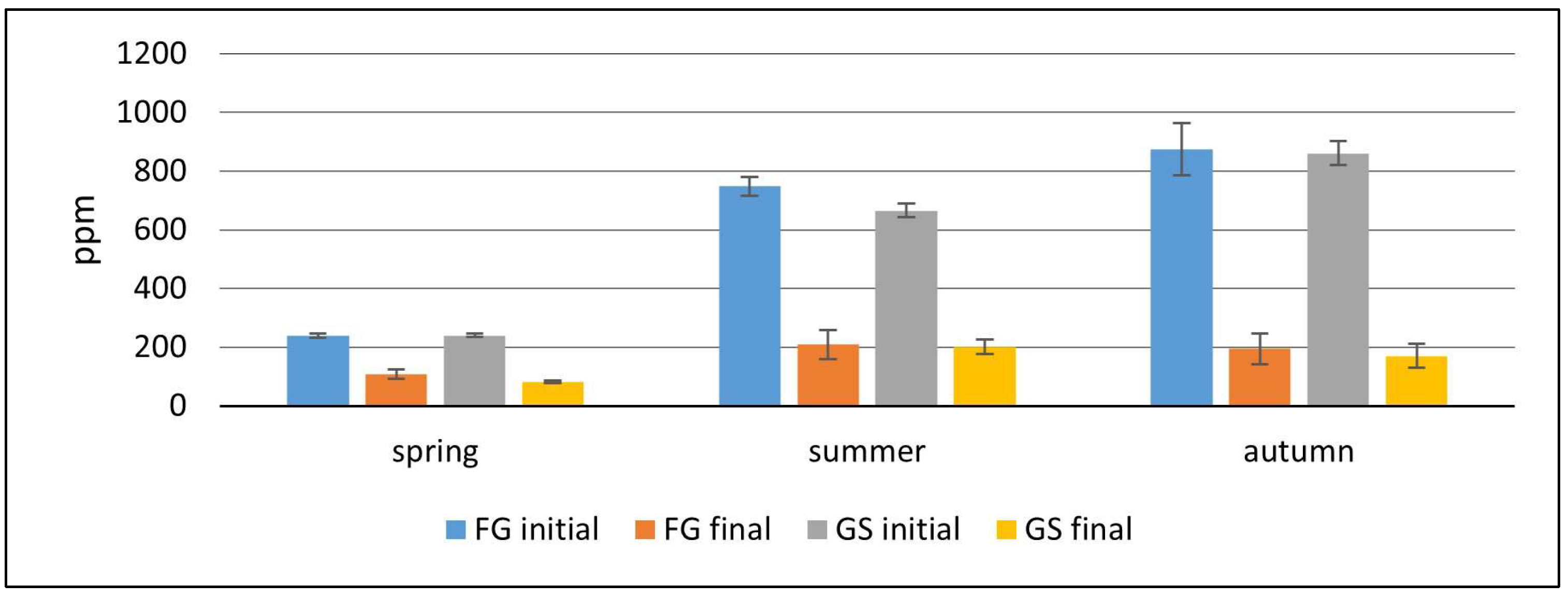
In addition to CH₄ and CO₂, biogas encompasses nitrogen (N₂), hydrogen (H₂), carbon monoxide (CO), oxygen (O₂), H₂S, and NH₃. The latter two compounds, released during the digestion of feedstock, may exhibit inhibitory effects on biogas production. The H₂S content in biogas is contingent upon the feedstock and AD technology, fluctuating between 2 and 12,000 ppm [61,62,63]. Elevated concentrations of H₂S result from the decomposition of sulphur-containing compounds, such as amino acids, sulphoxides, sulphonic acids, and the biological reduction of sulphates in the feedstock [64].

The presence of H₂S not only hampers the AD process by denaturing proteins in microorganisms responsible for feedstock digestion, but also leads to the formation of a corrosive condensate with water in biogas, causing damage to combined heat and power (CHP) units and installations [65,66]. The toxicity of sulphur oxides (SOx) released into the atmosphere [65,67] and the corrosion of installations or engine damage in biogas plants compel operators to eliminate H₂S from biogas. However, the threshold value is contingent not only on the safety of the biogas installation but also on its subsequent applications. In biogas used in microturbines, the threshold value is high (70,000 ppm); in CHP units, the acceptable range is between 100 and 500 ppm [67,68], and biogas upgraded to biomethane should contain 4–10 ppm [69].

In this study, the initial H₂S concentrations for summer- and autumn-cut grass exceeded the threshold values for CHP units, whereas the H₂S concentration in biogas from spring-cut grass remained very low, even at the beginning of the experiment. Similar disparities in H₂S concentration, influenced by cutting time, were reported by Chumenti et al. [25], who observed a significantly higher H₂S content in biogas produced from summer-cut grass compared to biogas from spring-cut grass. Chumenti et al. [70] also reported significant differences in H₂S concentrations in biogas produced from fresh and ensiled grass, contradicting the results of this study. Studies by Żurek and Martyniak [47] indicated relatively low H₂S concentrations in biogas from perennial grasses, ranging from 272 to 298 ppm.

Another studied inhibitor is produced during the AD process. NH₄⁺ is released through the degradation of nitrogen-rich compounds, primarily proteins, urea, and nucleic acids [64,71,72,73]. This compound is not degraded under anaerobic conditions and is in equilibrium with NH₃, whose concentration is influenced by pH and temperature. A decrease in pH may lead to an increase in NH₃ concentration, adversely affecting the community structure of archaea, which is responsible for CH₄ production, and consequently reducing CH₄ yield [74]. Inhibition of archaea leads to an increase in Volatile Fatty Acids (VFA) and a reduction in pH value [75]. Threshold values for NH₃ concentration range from 80 to 400 ppm [76]; however, the toxicity limits in the literature vary significantly, ranging from 60 to 14,000 ppm [64,77]. In this study, even the highest NH₃ value was lower than the threshold value and decreased significantly by the end of the experiment.

The compositional analysis of grass identified predominant FAMEs such as C16:0, C18:0, C18:1n9t/c, C18:2n6c, and C18:3n6, which are considered suitable for fuel production. Synthesised biodiesel, as reported in the literature, demonstrated the highest yield when derived from waste cooking oil (80.6%), followed by a mix of waste cooking oil and animal fats (79.3%). Characterisation of the produced biodiesel revealed the presence of various FAMEs components, with oleic acid (C18:1n9c), palmitic acid (C16:0), and linoleic acid (C18:2n6c) identified as major constituents [78]. Spectroscopic studies assessing the quality of FAMEs obtained from waste cooking oil confirmed their compliance with the European Standard EN 14214:2006 requirements [79]. FAMEs extracted from spent coffee grounds exhibited a composition composed of C16:0 (41.7%) and C18:0 (48.2%), rendering these extracts suitable for conversion into biodiesel. Furthermore, the residual solid fraction resulting from lignin and FAME extraction underwent AD under mesophilic conditions, yielding CH₄ at a rate of 360 NL kg_VS⁻¹ [37]. The FAME composition derived from cherry stone waste indicated a notable unsaturated to saturated fatty acid ratio [38]. Similarly, herbal waste exhibited higher amounts of unsaturated FAMEs compared to saturated ones, with linoleic acid identified as the major polyunsaturated FAME and palmitic acid as the major saturated FAME [39].

The comparative analysis of the compositional profiles between the examined grass samples and other waste materials, such as municipal sewage sludge [80], revealed analogous distributions of FAMEs. Palmitic acid (C16:0) emerged as the predominant saturated fatty acid, constituting 37.5%, followed by stearic acid (C18:0) at 12.0%. Oleic acid (C18:1n9c) dominated the unsaturated fatty acids, accounting for 29.0%, while linoleic acid (C18:2n6c) represented 6.2% of the total FAMEs. Similarly, in lipids extracted from primary sludge, Villalobos-Delgado et al. [81] identified palmitic acid (C16:0) as the major saturated fatty acid (42–58%), trailed by stearic acid (C18:0) at 18.3–24.5%, and oleic (C18:1n9c) and linoleic (C18:2n6c) acids at 9.5–22.3%.

The concentration of total FAMEs in the grass samples varied from 98.08 mg g_DM⁻¹ in FG-Au to 56.37 mg g_DM⁻¹ in FG-Sp. Notably, the C16:0 fatty acid ranged from 37.82 to 66.87 mg g_DM⁻¹, and C18:0 from 4.50 to 6.83 mg g_DM⁻¹, constituting the most abundant components. These specific FAMEs are considered ideal for biofuel production. In comparison, integrated processes for food waste yielded 248.21 g of FAMEs per 1 kg [82]. Similarly, high lipid concentrations (248 mg g_DM⁻¹) were observed in Chlorella vulgaris [83], highlighting the advantage of microalgae biomass production from waste in a more spatially efficient manner than other crop types. In herbal waste, the highest total FAMEs concentration was observed in rye bran (35.79 mg g_DM⁻¹), herbal tea (11.69 mg g_DM⁻¹), and chicory (8.78 mg g_DM⁻¹), with the majority of herbal waste (62.5%) falling within the total FAMEs content range of 1.42 to 5.02 mg g_DM⁻¹ [39].

The lipid content in temperate grasses is relatively low and tends to decrease as the plant matures [84]. The highest concentration of total FAMEs was observed in fresh grass samples collected in autumn and summer, with values of 98.08 mg g_DM⁻¹ and 90.03 mg g_DM⁻¹, respectively. Whetsell and Rayburn [85] highlighted that vegetative growth and leafiness significantly influence the Fatty Acid (FA) content in grasses, emphasising the negative impact of summer months, specifically May, June, and July, on total FA content. Furthermore, the total FA content exhibited a stronger correlation with linolenic acid (C18:3) than with linoleic acid (C18:2), with lower correlations observed between linoleic acid (C18:2) and linolenic acid (C18:3) content. Concentrations of linoleic acid (C18:2), linolenic acid (C18:3), and total FAs were higher during the summer compared to spring growth [86]. Consistent with these findings, the present study reported the lowest concentration of total FAMEs in FS-Sp (56.37 mg g_DM⁻¹) and GS-Sp (58.42 mg g_DM⁻¹). Intriguingly, GS-Sp exhibited a higher content of these compounds than FG-Sp.

The ensiling process significantly influenced the content of total FAMEs in spring grass, resulting in a reduction in total saturated fatty acids and an increase in total unsaturated fatty acids. These results are in good agreement with the findings of Khan et al. [87], who attributed variations in plant maturity at harvest as the primary explanation for the variability in FA content, highlighting higher contents of C18:3n3 in silages from young grass. Notably, the FAMEs content in grass silage from summer and autumn was lower than in fresh grass from these cutting times. The highest concentration of total FAMEs in ensiled grass (75.81 mg g_DM⁻¹) was detected in samples from summer, closely related to the dry matter content in the analysed samples.

Biodiesel production from waste oils presents challenges, including elevated Free Fatty Acids (FFA) during transesterification. The presence of FFA and water leads to the formation of glycerol (propane-1,2,3-triol) as a by-product and reduces methyl ester levels [88]. The amount of glycerol is contingent on the conversion methods, as well as the type of alcohol and catalyst employed [89]. A substantial portion (70–95%) of the total biodiesel production cost is associated with raw materials [90]. Utilising waste materials, such as waste cooking oil, can significantly reduce production costs, with the cost of obtaining waste cooking oil being 2.5 to 3.5 times lower than that of edible vegetable oils [91]. Osman et al. [92] have explored computational and machine learning techniques, biodiesel characteristics, transesterification processes, waste materials, and policies encouraging biodiesel production from waste. Consequently, the studied grasses represent a potential source for biodiesel production. However, further investigations into their properties are needed.

Although the studied grass exhibits potential for application in both biodiesel and biogas production, its limited availability results in a low energy yield per hectare [51]. Hence, grass waste from the maintenance of road verges should not be viewed as the primary substrate for the production of liquid or gaseous biofuels. Instead, it should be considered a supplementary feedstock, to be used alongside other resources that are available in quantities sufficient for the operations of biofuel plants. The findings underscore the potential for alternative utilisation of biowaste, thereby prompting consideration for future policy adjustments in urban waste management strategies, integrating energy generation in alignment with the principles of circular economy.

5. Conclusions

The results of this study confirmed the suitability of grass biomass collected during road verges maintenance of for the production of both liquid and gaseous biofuels. Considering the total energy content of the produced biofuels, the biogas production proved to be more efficient than biodiesel production. An additional aspect favouring this direction of utilising the analysed substrates is the potential for both electricity and heat production. On the other hand, the fact that grass from road verges is also suitable for biodiesel production makes it a versatile feedstock for various types of biofuels. However, it should be noted that the analysed type of biomass, due to its properties, is often a challenging feedstock and cannot be considered as the primary substrate for biogas production. The conducted research, nevertheless, demonstrated that its application should not negatively impact the methanogenic fermentation process. Regarding the produced biodiesel, additional studies are necessary to demonstrate its actual suitability as a transportation fuel.

Author Contributions

Conceptualisation, R.C., A.W.-C. and A.S.; methodology, R.C., A.W.-C., A.S., A.P.-N. and A.B.; formal analysis, R.C., A.W.-C., A.S., A.P.-N. and A.B.; investigation, R.C., A.W.-C., A.S., A.P.-N. and A.B.; writing—original draft preparation, R.C., A.W.-C. and A.S.; writing—review and editing, R.C., A.W.-C., A.S., A.P.-N., M.J.W. and A.B.; visualisation, R.C. and A.S. All authors have read and agreed to the published version of the manuscript.

Funding

This work was financially supported by the Ministry of Science and Higher Education as part of the project WZ/WB-IIŚ/3/2023 and this work was funded by the Ministry of Science and Higher Education as part of the subsidies to maintain research potential awarded to the Faculty of Biology of the University of Bialystok (SWB-3).

Data Availability Statement

Data are contained within the article.

Conflicts of Interest

The authors declare no conflicts of interest. The funders had no role in the design of the study; in the collection, analyses, or interpretation of data; in the writing of the manuscript; or in the decision to publish the results.

References

United Nations Environment Programme. Global Material Flows and Resource Productivity: Assessment Report for the UNEP International Resource Panel, 1st ed.; United Nations Environment Programme: Paris, France, 2016. [Google Scholar]
World Economic Forum. BiodiverCities by 2030: Transforming Cities’ Relationship with Nature, 1st ed.; World Economic Forum: Cologny/Geneva, Switzerland, 2022. [Google Scholar]
United Nations Environment Programme. Sustainable Cities. Available online: http://www.unep.org/regions/asia-and-pacific/regional-initiatives/supporting-resource-efficiency/sustainable-cities (accessed on 6 May 2023).
United Nations, Department of Economic and Social Affairs, Population Division. World Urbanization Prospects 2018: Highlights (ST/ESA/SER.A/421), 1st ed.; United Nations: New York, NY, USA, 2019. [Google Scholar]
European Environmental Agency. Urban Sustainability. Available online: https://www.eea.europa.eu/en/topics/in-depth/urban-sustainability (accessed on 6 May 2023).
United Nations General Assembly. A/RES/70/1 Transforming Our World: The 2030 Agenda for Sustainable Development; United Nations General Assembly: New York, NY, USA, 2015. [Google Scholar]
European Commission. The European Green Deal. Communication from the Commission to the European Parliament, the European Council, the Council, the European Economic and Social Committee and the Committee of the Regions. COM(2019) 640 Final; European Commision: Brussels, Belgium, 2019. [Google Scholar]
Journal of Laws 2004 No. 92/880 Nature Conservation Act of April 2004 (In Polish). Available online: https://isap.sejm.gov.pl/isap.nsf/download.xsp/WDU20040920880/U/D20040880Lj.pdf (accessed on 6 May 2023).
Khoshtaria, T.K.; Chachava, N.T. The Planning of Urban Green Areas and Its Protective Importance in Resort Cities (Case of Georgian Resorts). Ann. Agrar. Sci. 2017, 15, 217–223. [Google Scholar] [CrossRef]
Bai, T.; Mayer, A.L.; Shuster, W.D.; Tian, G. The Hydrologic Role of Urban Green Space in Mitigating Flooding (Luohe, China). Sustainability 2018, 10, 3584. [Google Scholar] [CrossRef]
Pascal, M.; Laaidi, K.; Beaudeau, P. Relevance of green, shaded environments in the prevention of adverse effects on health from heat and air pollution in urban areas. Sante Publique 2019, S1, 197–205. [Google Scholar] [CrossRef]
Wang, W.; Liu, K.; Tang, R.; Wang, S. Remote Sensing Image-Based Analysis of the Urban Heat Island Effect in Shenzhen, China. Phys. Chem. Earth Parts A/B/C 2019, 110, 168–175. [Google Scholar] [CrossRef]
Kumar, P.; Debele, S.E.; Khalili, S.; Halios, C.H.; Sahani, J.; Aghamohammadi, N.; Andrade, M.D.F.; Athanassiadou, M.; Bhui, K.; Calvillo, N.; et al. Urban Heat Mitigation by Green and Blue Infrastructure: Drivers, Effectiveness, and Future Needs. Innovation 2024, 5, 100588. [Google Scholar] [CrossRef] [PubMed]
Starczewski, T.; Rogatka, K.; Kukulska-Kozieł, A.; Noszczyk, T.; Cegielska, K. Urban Green Resilience: Experience from Post-Industrial Cities in Poland. Geosci. Front. 2023, 14, 101560. [Google Scholar] [CrossRef]
Caprotti, F.; Springer, C.; Harmer, N. ‘Eco’ For Whom? Envisioning Eco-Urbanism in the Sino-Singapore Tianjin Eco-City, China. Int. J. Urban Reg. Res. 2015, 39, 495–517. [Google Scholar] [CrossRef]
Hitchmough, J.; Fieldhouse, K. Plant User Handbook: A Guide to Effective Specifying, 1st ed.; Wiley-Blackwell: Oxford, UK; Malden, MA, USA; Carlton, VIC, Australia, 2003. [Google Scholar]
Li, N.; Liu, Y. Sustainable Design in Urban Green Space. In Sustainability in Urban Planning and Design; Almusaed, A., Almssad, A., Truong-Hong, L., Eds.; IntechOpen: London, UK, 2020. [Google Scholar]
Ansari, S.A.; Shakeel, A.; Sawarkar, R.; Maddalwar, S.; Khan, D.; Singh, L. Additive Facilitated Co-Composting of Lignocellulosic Biomass Waste, Approach towards Minimizing Greenhouse Gas Emissions: An up to Date Review. Environ. Res. 2023, 224, 115529. [Google Scholar] [CrossRef] [PubMed]
Bedoić, R.; Čuček, L.; Ćosić, B.; Krajnc, D.; Smoljanić, G.; Kravanja, Z.; Ljubas, D.; Pukšec, T.; Duić, N. Green Biomass to Biogas–A Study on Anaerobic Digestion of Residue Grass. J. Clean. Prod. 2019, 213, 700–709. [Google Scholar] [CrossRef]
Seppälä, M.; Paavola, T.; Lehtomäki, A.; Rintala, J. Biogas Production from Boreal Herbaceous Grasses–Specific Methane Yield and Methane Yield per Hectare. Bioresour. Technol. 2009, 100, 2952–2958. [Google Scholar] [CrossRef]
McEniry, J.; O’Kiely, P. Anaerobic Methane Production from Five Common Grassland Species at Sequential Stages of Maturity. Bioresour. Technol. 2013, 127, 143–150. [Google Scholar] [CrossRef] [PubMed]
Cadavid-Rodríguez, L.S.; Bolaños-Valencia, I.V. Grass from Public Green Spaces an Alternative Source of Renewable Energy in Tropical Countries. Rev. ION 2016, 29, 109–116. [Google Scholar] [CrossRef]
Piepenschneider, M.; Bühle, L.; Hensgen, F.; Wachendorf, M. Energy Recovery from Grass of Urban Roadside Verges by Anaerobic Digestion and Combustion after Pre-Processing. Biomass Bioenerg. 2016, 85, 278–287. [Google Scholar] [CrossRef]
Dragoni, F.; Giannini, V.; Ragaglini, G.; Bonari, E.; Silvestri, N. Effect of Harvest Time and Frequency on Biomass Quality and Biomethane Potential of Common Reed (Phragmites Australis) Under Paludiculture Conditions. Bioenerg. Res. 2017, 10, 1066–1078. [Google Scholar] [CrossRef]
Chiumenti, A.; Boscaro, D.; Da Borso, F.; Sartori, L.; Pezzuolo, A. Biogas from Fresh Spring and Summer Grass: Effect of the Harvesting Period. Energies 2018, 11, 1466. [Google Scholar] [CrossRef]
Roj-Rojewski, S.; Wysocka-Czubaszek, A.; Czubaszek, R.; Kamocki, A.; Banaszuk, P. Anaerobic Digestion of Wetland Biomass from Conservation Management for Biogas Production. Biomass Bioenerg. 2019, 122, 126–132. [Google Scholar] [CrossRef]
De Moor, S.; Velghe, F.; Wierinck, I.; Michels, E.; Ryckaert, B.; De Vocht, A.; Verbeke, W.; Meers, E. Feasibility of Grass Co-Digestion in an Agricultural Digester, Influence on Process Parameters and Residue Composition. Bioresour. Technol. 2013, 150, 187–194. [Google Scholar] [CrossRef]
Poulsen, T.G.; Adelard, L. Improving Biogas Quality and Methane Yield via Co-Digestion of Agricultural and Urban Biomass Wastes. Waste. Manag. 2016, 54, 118–125. [Google Scholar] [CrossRef] [PubMed]
Prochnow, A.; Heiermann, M.; Plöchl, M.; Linke, B.; Idler, C.; Amon, T.; Hobbs, P.J. Bioenergy from Permanent Grassland–A Review: 1. Biogas. Bioresour. Technol. 2009, 100, 4931–4944. [Google Scholar] [CrossRef]
Alvarez Serafini, M.S.; Tonetto, G.M. Production of Fatty Acid Methyl Esters from an Olive Oil Industry Waste. Braz. J. Chem. Eng. 2019, 36, 285–297. [Google Scholar] [CrossRef]
Olutoye, M.A.; Hameed, B.H. A Highly Active Clay-Based Catalyst for the Synthesis of Fatty Acid Methyl Ester from Waste Cooking Palm Oil. Appl. Catal. A General 2013, 450, 57–62. [Google Scholar] [CrossRef]
García-Morales, R.; Zúñiga-Moreno, A.; Verónico-Sánchez, F.J.; Domenzain-González, J.; Pérez-López, H.I.; Bouchot, C.; Elizalde-Solis, O. Fatty Acid Methyl Esters from Waste Beef Tallow Using Supercritical Methanol Transesterification. Fuel 2022, 313, 122706. [Google Scholar] [CrossRef]
Golmakani, M.-T.; Moosavi-Nasab, M.; Raayatpisheh, M.; Dehghani, Z. Fatty Acid Methyl Ester Production from Rainbow Trout Waste Oil Using Microwave-Assisted Transesterification. Process Biochem. 2024, 139, 33–43. [Google Scholar] [CrossRef]
Dube, A.S. Synthesis of Chicken Fat Methyl Ester. IJRASET 2018, 6, 2223–2227. [Google Scholar] [CrossRef]
Cruz, A.G.; Mtz-Enríquez, A.I.; Díaz-Jiménez, L.; Ramos-González, R.; Valdés, J.A.A.; Flores, M.E.C.; Martínez, J.L.H.; Ilyina, A. Production of Fatty Acid Methyl Esters and Bioactive Compounds from Citrus Wax. Waste Manag. 2020, 102, 48–55. [Google Scholar] [CrossRef]
Magalhães-Ghiotto, G.A.V.; Marcucci, S.M.P.; Trevisan, E.; Arroyo, P.A. Extraction and Characterization of the Lipids from Domestic Sewage Sludge and in Situ Synthesis of Methyl Esters. Environ. Prog. Sustain. Energy 2023, 42, e14027. [Google Scholar] [CrossRef]
Lee, M.; Yang, M.; Choi, S.; Shin, J.; Park, C.; Cho, S.-K.; Kim, Y.M. Sequential Production of Lignin, Fatty Acid Methyl Esters and Biogas from Spent Coffee Grounds via an Integrated Physicochemical and Biological Process. Energies 2019, 12, 2360. [Google Scholar] [CrossRef]
Kniepkamp, K.; Errico, M.; Yu, M.; Roda-Serrat, M.C.; Eilers, J.-G.; Wark, M.; van Haren, R. Lipid Extraction of High-Moisture Sour Cherry (Prunus Cerasus L.) Stones by Supercritical Carbon Dioxide. J. Chem. Technol. Biotechnol. 2024, 99, 810–819. [Google Scholar] [CrossRef]
Sienkiewicz, A.; Piotrowska-Niczyporuk, A.; Bajguz, A. Fatty Acid Methyl Esters from the Herbal Industry Wastes as a Potential Feedstock for Biodiesel Production. Energies 2020, 13, 3702. [Google Scholar] [CrossRef]
Statistical Office in Białystok. Available online: https://bialystok.stat.gov.pl/en/ (accessed on 20 February 2024).
Górniak, A. Climate of the Podlaskie Voivodeship in the Time of Global Warming (In Polish), 1st ed.; Wydawnictwo Uniwersytetu w Białymstoku: Białystok, Poland, 2021. [Google Scholar]
Wang, K.; Yun, S.; Xing, T.; Li, B.; Abbas, Y.; Liu, X. Binary and Ternary Trace Elements to Enhance Anaerobic Digestion of Cattle Manure: Focusing on Kinetic Models for Biogas Production and Digestate Utilization. Bioresour. Technol. 2021, 323, 124571. [Google Scholar] [CrossRef]
Journal of Laws 2020. Regulation of the Minister of Climate of July 11, 2020 on the Calorific Value of Individual Biocomponents and Liquid Fuels (In Polish). Available online: https://isap.sejm.gov.pl/isap.nsf/download.xsp/WDU20200001278/O/D20201278.pdf (accessed on 8 September 2023).
The National Centre for Emissions Management. Emission Factors for CO2, SO2, NOx and Total Particulate Matter for Electrical Energy on the Basis of Information in National Database on Emissions of Greenhouse Gases and Other Substances for 2020 (In Polish); The National Centre for Emissions Management: Warsaw, Poland, 2020. [Google Scholar]
The National Centre for Emissions Management. Calorific Values (CO) and CO2 Emission Factors (EC) in 2019 to Be Reported under the Emission Trading Scheme for 2022; The National Centre for Emissions Management: Warsaw, Poland, 2021. [Google Scholar]
Rajendran, K.; Aslanzadeh, S.; Taherzadeh, M.J. Household Biogas Digesters—A Review. Energies 2012, 5, 2911–2942. [Google Scholar] [CrossRef]
Żurek, G.; Martyniak, M. The Biogas Potential of Selected Perennial Grasses from Genus Bromus. Biul. IHAR 2020, 289, 3–10. [Google Scholar] [CrossRef]
Triolo, J.M.; Pedersen, L.; Qu, H.; Sommer, S.G. Biochemical Methane Potential and Anaerobic Biodegradability of Non-Herbaceous and Herbaceous Phytomass in Biogas Production. Bioresour. Technol. 2012, 125, 226–232. [Google Scholar] [CrossRef] [PubMed]
Korres, N.E.; Thamsiriroj, T.; Smyth, B.M.; Nizami, A.S.; Singh, A.; Murphy, J.D. Grass Biomethane for Agriculture and Energy. In Genetics, Biofuels and Local Farming Systems; Lichtfouse, E., Ed.; Sustainable Agriculture Reviews; Springer: Dordrecht, The Netherlands, 2011; pp. 5–49. ISBN 978-94-007-1521-9. [Google Scholar]
Weiland, P. Biomass Digestion in Agriculture: A Successful Pathway for the Energy Production and Waste Treatment in Germany. Eng. Life Sci. 2006, 6, 302–309. [Google Scholar] [CrossRef]
Czubaszek, R.; Wysocka-Czubaszek, A.; Banaszuk, P.; Zając, G.; Wassen, M.J. Grass from Road Verges as a Substrate for Biogas Production. Energies 2023, 16, 4488. [Google Scholar] [CrossRef]
Nizami, A.-S.; Korres, N.E.; Murphy, J.D. Review of the Integrated Process for the Production of Grass Biomethane. Environ. Sci. Technol. 2009, 43, 8496–8508. [Google Scholar] [CrossRef] [PubMed]
Cui, X.; Sun, H.; Sobhi, M.; Ju, X.; Guo, J.; Dong, R. Butyric Acid Fermentation during Ensiling of Wilted Maize Stover for Efficient Methane Production. ACS Sustainable Chem. Eng. 2020, 8, 6713–6721. [Google Scholar] [CrossRef]
Feng, L.; Kristensen, E.F.; Moset, V.; Ward, A.J.; Møller, H.B. Ensiling of Tall Fescue for Biogas Production: Effect of Storage Time, Additives and Mechanical Pretreatment. Energy Sustain. Dev. 2018, 47, 143–148. [Google Scholar] [CrossRef]
Hillion, M.-L.; Moscoviz, R.; Trably, E.; Leblanc, Y.; Bernet, N.; Torrijos, M.; Escudié, R. Co-Ensiling as a New Technique for Long-Term Storage of Agro-Industrial Waste with Low Sugar Content Prior to Anaerobic Digestion. Waste Manag. 2018, 71, 147–155. [Google Scholar] [CrossRef]
Menardo, S.; Balsari, P.; Tabacco, E.; Borreani, G. Effect of Conservation Time and the Addition of Lactic Acid Bacteria on the Biogas and Methane Production of Corn Stalk Silage. Bioenerg. Res. 2015, 8, 1810–1823. [Google Scholar] [CrossRef]
Liu, S.; Ge, X.; Liew, L.N.; Liu, Z.; Li, Y. Effect of Urea Addition on Giant Reed Ensilage and Subsequent Methane Production by Anaerobic Digestion. Bioresour. Technol. 2015, 192, 682–688. [Google Scholar] [CrossRef] [PubMed]
Sun, H.; Cui, X.; Li, R.; Guo, J.; Dong, R. Ensiling Process for Efficient Biogas Production from Lignocellulosic Substrates: Methods, Mechanisms, and Measures. Bioresour. Technol. 2021, 342, 125928. [Google Scholar] [CrossRef]
Herrmann, C.; Heiermann, M.; Idler, C. Effects of Ensiling, Silage Additives and Storage Period on Methane Formation of Biogas Crops. Bioresour. Technol. 2011, 102, 5153–5161. [Google Scholar] [CrossRef] [PubMed]
Teixeira Franco, R.; Buffière, P.; Bayard, R. Ensiling for Biogas Production: Critical Parameters. A Review. Biomass Bioenerg. 2016, 94, 94–104. [Google Scholar] [CrossRef]
Fortuny, M.; Baeza, J.A.; Gamisans, X.; Casas, C.; Lafuente, J.; Deshusses, M.A.; Gabriel, D. Biological Sweetening of Energy Gases Mimics in Biotrickling Filters. Chemosphere 2008, 71, 10–17. [Google Scholar] [CrossRef] [PubMed]
Mamun, M.R.A.; Torii, S. Removal of Hydrogen Sulfide (H₂S) from Biogas Using Zero-Valent Iron. J. Clean Energy Technol. 2015, 3, 428–432. [Google Scholar] [CrossRef]
Calbry-Muzyka, A.; Madi, H.; Rüsch-Pfund, F.; Gandiglio, M.; Biollaz, S. Biogas Composition from Agricultural Sources and Organic Fraction of Municipal Solid Waste. Renew. Energy 2022, 181, 1000–1007. [Google Scholar] [CrossRef]
Chen, Y.; Cheng, J.J.; Creamer, K.S. Inhibition of Anaerobic Digestion Process: A Review. Bioresour. Technol. 2008, 99, 4044–4064. [Google Scholar] [CrossRef] [PubMed]
Żarczyński, A.; Rosiak, K.; Anielak, P.; Wolf, W. Practical Methods of Cleaning Biogas from Hydrogen Sulphide. Part 1. Application of Solid Sorbents. Acta Innov. 2014, 12, 24–34. [Google Scholar]
Czatzkowska, M.; Harnisz, M.; Korzeniewska, E.; Koniuszewska, I. Inhibitors of the Methane Fermentation Process with Particular Emphasis on the Microbiological Aspect: A Review. Energy. Sci. Eng. 2020, 8, 1880–1897. [Google Scholar] [CrossRef]
Aita, B.C.; Mayer, F.D.; Muratt, D.T.; Brondani, M.; Pujol, S.B.; Denardi, L.B.; Hoffmann, R.; da Silveira, D.D. Biofiltration of H₂S-Rich Biogas Using Acidithiobacillus Thiooxidans. Clean. Technol. Environ. Policy 2016, 18, 689–703. [Google Scholar] [CrossRef]
Moreno-Andrade, I.; Moreno, G.; Quijano, G. Theoretical Framework for the Estimation of H₂S Concentration in Biogas Produced from Complex Sulfur-Rich Substrates. Environ. Sci. Pollut. Res. 2020, 27, 15959–15966. [Google Scholar] [CrossRef] [PubMed]
Jung, H.; Kim, D.; Choi, H.; Lee, C. A Review of Technologies for In-Situ Sulfide Control in Anaerobic Digestion. Renew. Sust. Energ. Rev. 2022, 157, 112068. [Google Scholar] [CrossRef]
Chiumenti, A.; Pezzuolo, A.; Boscaro, D.; da Borso, F. Exploitation of Mowed Grass from Green Areas by Means of Anaerobic Digestion: Effects of Grass Conservation Methods (Drying and Ensiling) on Biogas and Biomethane Yield. Energies 2019, 12, 3244. [Google Scholar] [CrossRef]
Rajagopal, R.; Massé, D.I.; Singh, G. A Critical Review on Inhibition of Anaerobic Digestion Process by Excess Ammonia. Bioresour. Technol. 2013, 143, 632–641. [Google Scholar] [CrossRef]
Westerholm, M.; Moestedt, J.; Schnürer, A. Biogas Production through Syntrophic Acetate Oxidation and Deliberate Operating Strategies for Improved Digester Performance. Appl. Energy 2016, 179, 124–135. [Google Scholar] [CrossRef]
Tian, H.; Fotidis, I.A.; Kissas, K.; Angelidaki, I. Effect of Different Ammonia Sources on Aceticlastic and Hydrogenotrophic Methanogens. Bioresour. Technol. 2018, 250, 390–397. [Google Scholar] [CrossRef]
Yang, Z.; Wang, W.; He, Y.; Zhang, R.; Liu, G. Effect of Ammonia on Methane Production, Methanogenesis Pathway, Microbial Community and Reactor Performance under Mesophilic and Thermophilic Conditions. Renew. Energy 2018, 125, 915–925. [Google Scholar] [CrossRef]
Kalamaras, S.D.; Vitoulis, G.; Christou, M.L.; Sfetsas, T.; Tziakas, S.; Fragos, V.; Samaras, P.; Kotsopoulos, T.A. The Effect of Ammonia Toxicity on Methane Production of a Full-Scale Biogas Plant—An Estimation Method. Energies 2021, 14, 5031. [Google Scholar] [CrossRef]
Theuerl, S.; Klang, J.; Prochnow, A. Process Disturbances in Agricultural Biogas Production—Causes, Mechanisms and Effects on the Biogas Microbiome: A Review. Energies 2019, 12, 365. [Google Scholar] [CrossRef]
Krakat, N.; Demirel, B.; Anjum, R.; Dietz, D. Methods of Ammonia Removal in Anaerobic Digestion: A Review. Water Sci. Technol. 2017, 76, 1925–1938. [Google Scholar] [CrossRef] [PubMed]
Al-Mawaali, S.; Al-Balushi, K.; Souissi, Y. Sustainable Biodiesel Production from Waste Cooking Oil and Waste Animal Fats. In Proceedings of the 8th World Congress on Civil, Structural, and Environmental Engineering, Lisbon, Portugal, 29−31 March 2023. [Google Scholar]
Matwijczuk, A.; Zając, G.; Karcz, D.; Chruściel, E.; Matwijczuk, A.; Kachel-Jakubowska, M.; Łapczyńska-Kordon, B.; Gagoś, M. Spectroscopic Studies of the Quality of WCO (Waste Cooking Oil) Fatty Acid Methyl Esters. BIO Web Conf. 2018, 10, 02019. [Google Scholar] [CrossRef]
Demirbas, A.; Bamufleh, H.; Gaber, G.; Al-Sasi, B.O. Biodiesel Production from Lipids of Municipal Sewage Sludge by Direct Methanol Transesterification. Energy Sources A REcovery Util. Environ. Eff. 2017, 39, 800–805. [Google Scholar] [CrossRef]
Villalobos-Delgado, F.d.J.; Reynel-Avila, H.E.; Mendoza-Castillo, D.I.; Bonilla-Petriciolet, A. Lipid Extraction in the Primary Sludge Generated from Urban Wastewater Treatment: Characteristics and Seasonal Composition Analysis. Water Sci. Technol. 2023, 87, 2930–2943. [Google Scholar] [CrossRef]
Patel, A.; Hrůzová, K.; Rova, U.; Christakopoulos, P.; Matsakas, L. Sustainable Biorefinery Concept for Biofuel Production through Holistic Volarization of Food Waste. Bioresour. Technol. 2019, 294, 122247. [Google Scholar] [CrossRef] [PubMed]
López-Pacheco, I.Y.; Ayala-Moreno, V.G.; Mejia-Melara, C.A.; Rodríguez-Rodríguez, J.; Cuellar-Bermudez, S.P.; González-González, R.B.; Coronado-Apodaca, K.G.; Farfan-Cabrera, L.I.; González-Meza, G.M.; Iqbal, H.M.N.; et al. Growth Behavior, Biomass Composition and Fatty Acid Methyl Esters (FAMEs) Production Potential of Chlamydomonas reinhardtii, and Chlorella vulgaris Cultures. Mar. Drugs. 2023, 21, 450. [Google Scholar] [CrossRef] [PubMed]
Frame, J.; Laidlaw, A.S. Improved Grassland Management, 2nd ed.; The Crowood Press: Ramsbury, UK, 2011. [Google Scholar]
Whetsell, M.; Rayburn, E. Variation in Fatty Acids Concentration in Grasses, Legumes, and Forbs in the Allegheny Plateau. Agronomy 2022, 12, 1693. [Google Scholar] [CrossRef]
Boufaïed, H.; Chouinard, P.Y.; Tremblay, G.F.; Petit, H.V.; Michaud, R.; Bélanger, G. Fatty Acids in Forages. II. In Vitro Ruminal Biohydrogenation of Linolenic and Linoleic Acids from Timothy. Can. J. Anim. Sci. 2003, 83, 513–522. [Google Scholar] [CrossRef]
Khan, N.A.; Cone, J.W.; Fievez, V.; Hendriks, W.H. Causes of Variation in Fatty Acid Content and Composition in Grass and Maize Silages. Anim. Feed Sci. Technol. 2012, 174, 36–45. [Google Scholar] [CrossRef]
Monika; Banga, S.; Pathak, V.V. Biodiesel Production from Waste Cooking Oil: A Comprehensive Review on the Application of Heterogenous Catalysts. Energy Nexus 2023, 10, 100209. [Google Scholar] [CrossRef]
Pitt, F.D.; Domingos, A.M.; Barros, A.A.C. Purification of Residual Glycerol Recovered from Biodiesel Production. S. Afr. J. Chem. Eng. 2019, 29, 42–51. [Google Scholar] [CrossRef]
Ahmia, A.C.; Danane, F.; Bessah, R.; Boumesbah, I. Raw Material for Biodiesel Production. Valorization of Used Edible Oil. J. Ren. Energ. 2023, 17, 335–343. [Google Scholar] [CrossRef]
Rehan, M.; Gardy, J.; Demirbas, A.; Rashid, U.; Budzianowski, W.M.; Pant, D.; Nizami, A.S. Waste to Biodiesel: A Preliminary Assessment for Saudi Arabia. Bioresour. Technol. 2018, 250, 17–25. [Google Scholar] [CrossRef]
Osman, A.I.; Nasr, M.; Farghali, M.; Rashwan, A.K.; Abdelkader, A.; Al-Muhtaseb, A.H.; Ihara, I.; Rooney, D.W. Optimizing Biodiesel Production from Waste with Computational Chemistry, Machine Learning and Policy Insights: A Review. Environ. Chem. Lett. 2024, 22, 1–67. [Google Scholar] [CrossRef]

Figure 1. Cumulative biogas production from fresh and ensiled grass cut in spring, summer, and autumn. FG—fresh grass; GS—grass silage. Standard deviations are shown as the vertical bars. Uppercase letters—significant difference among cutting time; lowercase letters—significant differences between preservation method.

Figure 2. Daily biogas production depending on cutting time: (a)—spring, (b)—summer, (c)—autumn and grass preservation method: (d)—fresh grass, (e)—grass silage. Standard deviations are shown as vertical bars. FG-Sp—spring fresh grass, GS-Sp—spring grass silage, FG-Su—summer fresh grass, GS-Su—summer grass silage, FG-Au—autumn fresh grass, GS-Au—autumn grass silage.

Figure 3. Cumulative biogas production depending on cutting time: (a)—spring, (b)—summer, (c)—autumn and grass preservation method: (d)—fresh grass, (e)—grass silage. Standard deviations are shown as vertical bars. The yellow squares and green squares represent T50 and T95, respectively. FG-Sp—spring fresh grass, GS-Sp—spring grass silage, FG-Su—summer fresh grass, GS-Su—summer grass silage, FG-Au—autumn fresh grass, GS-Au—autumn grass silage.

Figure 4. The initial and final concentration of the hydrogen sulphide (H₂S) in biogas produced from fresh and ensiled grass harvested in spring, summer, and autumn. Standard deviations are shown as vertical bars. FG—fresh grass, GS—grass silage.

Figure 5. The initial and final concentration of the ammonia (NH₃) in biogas produced from fresh and ensiled grass harvested in spring, summer, and autumn. Standard deviations are shown as vertical bars. FG—fresh grass, GS—grass silage.

Figure 6. FAMEs composition of fresh grass and ensiled grass harvested in spring, summer and autumn. FG-Sp—spring fresh grass, GS-Sp—spring grass silage, FG-Su—summer fresh grass, GS-Su—summer grass silage, FG-Au—autumn fresh grass, GS-Au—autumn grass silage.

Figure 7. Biplot of FAMEs content in grass samples, showing the first two principal components (PC1 and PC2) of the PCA model that together explain 61.8% of the total variance, i.e., 40.60% and 21.16% for PC1 and PC2, respectively. Blue biplot vectors indicate the strength and direction of factor loading for all analysed fatty acids. FG-Sp—spring fresh grass, GS-Sp—spring grass silage, FG-Su—summer fresh grass, GS-Su—summer grass silage, FG-Au—autumn fresh grass, GS-Au—autumn grass silage.

Table 1. Chemical composition (mean ± SD, n = 3) of fresh grass and grass silage from three cutting times.

Parameter	Spring		Summer		Autumn
	Fresh Grass	Grass Silage	Fresh Grass	Grass Silage	Fresh Grass	Grass Silage
	(FG-Sp)	(GS-Sp)	(FG-Su)	(GS-Su)	(FG-Au)	(GS-Au)
Total solids (TS), %	38.00 ± 1.35	37.37 ± 0.58	25.83 ± 0.97	29.11 ± 0.37	29.34 ± 0.97	30.33 ± 0.30
Volatile solids (VS), %TS	68.22 ± 7.98	67.93 ± 7.58	84.70 ± 1.32	83.34 ± 2.08	88.83 ± 0.10	87.69 ± 0.08
pH	6.17 ± 0.01	5.44 ± 0.03	5.96 ± 0.04	4.54 ± 0.03	5.97 ± 0.04	4.15 ± 0.02
Total Kieldahl nitrogen (TKN), g kg_DM⁻¹	20.76 ± 0.23	22.12 ± 0.63	25.89 ± 0.84	28.39 ± 0.67	27.67 ± 1.12	25.87 ± 0.34
Total phosphorus (TP), g kg_DM⁻¹	1.99 ± 0.19	2.32 ± 0.06	3.42 ± 0.26	3.72 ± 0.04	3.06 ± 0.05	3.55 ± 0.12
Potassium (K), g kg_DM⁻¹	10.96 ± 1.43	12.97 ± 1.12	23.48 ± 1.36	24.94 ± 0.35	15.00 ± 0.08	18.72 ± 0.46
Sodium (Na), g kg_DM⁻¹	3.12 ± 0.48	4.58 ± 0.41	0.85 ± 0.44	0.85 ± 0.10	n.d.	n.d.
Total organic carbon (TOC), g kg_DM⁻¹	373.80 ± 18.29	323.49 ± 63.45	371.63 ± 22.42	368.04 ± 8.66	381.87 ± 3.17	421.68 ± 14.38

n.d.—not detected.

Table 2. Chemical composition of inocula (mean ± SD; n = 3) used in three biochemical biogas potential (BBP) tests.

Parameter	Spring	Summer	Autumn
TS, %	4.58 ± 0.00	5.19 ± 0.02	4.76 ± 0.07
VS, %TS	77.41 ± 0.22	78.57 ± 0.21	76.11 ± 0.21
pH	8.11 ± 0.02	7.84 ± 0.05	8.19 ± 0.02
TKN, g kg_DM⁻¹	90.83 ± 4.63	90.53 ± 3.18	69.41 ± 1.05
TP, g kg_DM⁻¹	8.41 ± 0.14	8.06 ± 0.21	8.81 ± 0.35
K, g kg_DM⁻¹	57.12 ± 1.88	49.81 ± 2.06	59.69 ± 1.90
Na, g kg_DM⁻¹	7.40 ± 0.29	5.69 ± 0.33	7.20 ± 0.28
TOC, g kg_DM⁻¹	433.53 ± 13.49	389.23 ± 6.00	421.53 ± 13.25

Table 3. Fatty Acid Methyl Esters standards used in the GC-MS analysis of grass samples.

Type of FAME	Systematic Name	The Common Name of FAME	Abbreviation
MUFA	Myristoleic acid methyl ester	Myristoleic acid	C14:1
	cis-10-Pentadecanoic acid methyl ester	Pentadecanoic acid	C15:1
	9-Hexadecenoic acid methyl ester	Palmitoleic acid	C16:1
	cis-10-Heptadecenoic acid methyl ester	Heptadecenoic acid	C17:1
	trans-9-Octadecenoic acid methyl ester (Z)	Elaidic acid	C18:1n9t
	9-Octadecenoic acid methyl ester (E)	Oleic acid	C18:1n9c
	cis-11-Eicosenoic acid methyl ester	Gondoic acid	C20:1
	13-Docosenoic acid methyl ester (Z)	Erucic acid	C22:1n9
	15-Tetracosenoic acid methyl ester (Z)	Nervonic acid	C24:1n9
PUFA	9,12-Octadecadienoic acid methyl ester (E,E)	Linolelaidic acid	C18:2n6t
	9,12-Octadecadienoic acid methyl ester (Z,Z)	Linoleic acid	C18:2n6c
	all-cis-6,9,12-Octadecatrienoic acid	γ-Linolenic acid	C18:3n6
	9,12,15-Octadecatrienoic acid methyl ester (Z,Z,Z)	Linolenic acid	C18:3n3
	cis-11,14-Eicosadienoic acid methyl ester	Eicosadienoic acid	C20:2
	cis-11,14,17-Eicosatrienoic acid methyl ester	Eicosatrienoic acid	C20:3n3
	cis-8,11,14-Eicosatrienoic acid methyl ester	Dihomo-γ-linolenic acid	C20:3n6
	5,8,11,14-Eicosatetraenoic acid methyl ester (all-Z)	Arachidonic acid	C20:4n6
	cis-5,8,11,14,17-Eicosapentaenoic acid methyl ester	Eicosapentaenoic acid	C20:5n3
	cis-13,16-Docasadienoic acid methyl ester	Docosadienoic acid	C22:2n6
	4,7,10,13,16,19-Docosahexaenoic acid methyl ester (all-Z)	Cervonic acid	C22:6n3
SFA	Butyric acid methyl ester	Butyric acid	C4:0
	Hexanoic acid methyl ester	Caproic acid	C6:0
	Octanoic acid methyl ester	Caprylic acid	C8:0
	Decanoic acid methyl ester	Capric acid	C10:0
	Undecanoic acid methyl ester	Undecylic acid	C11:0
	Dodecanoic acid methyl ester	Lauric acid	C12:0
	Tridecanoic acid methyl ester	Tridecylic acid	C13:0
	Tetradecanoic acid methyl ester	Myristic acid	C14:0
	Pentadecanoic acid methyl ester	Pentadecylic acid	C15:0
	Hexadecanoic acid methyl ester	Palmitic acid	C16:0
	Heptadecanoic acid methyl ester	Margaric acid	C17:0
	Octadecanoic acid methyl ester	Stearic acid	C18:0
	Eicosanoic acid methyl ester	Arachidic acid	C20:0
	Heneicosanoic acid methyl ester	Heneicosylic acid	C21:0
	Docosanoic acid methyl ester	Behenic acid	C22:0
	Tricosanoic acid methyl ester	Tricosylic acid	C23:0
	Tetracosanoic acid methyl ester	Lignoceric acid	C24:0

MUFA—monounsaturated fatty acid, PUFA—polyunsaturated fatty acid, SFA—saturated fatty acid.

Table 4. Methane (CH₄) concentration (mean ± SD; n = 3) in the produced biogas depending on the method of grass preservation and the cutting time.

Season	Fresh Grass	Grass Silage
	%
Spring	59.7 ± 0.6 Aa	60.0 ± 1.0 Aa
Summer	58.7 ± 1.2 Aa	58.0 ± 1.0 Aa
Autumn	55.7 ± 1.5 Ba	55.0 ± 2.0 Ba

Uppercase letters—significant difference among cutting time; lowercase letters—significant differences between preservation methods.

Table 5. The content of monounsaturated fatty acids (mean ± SD, n = 3) in fresh grass and ensiled grass cut in spring, summer, and autumn.

MUFA	Spring		Summer		Autumn
MUFA	Fresh Grass	Grass Silage	Fresh Grass	Grass Silage	Fresh Grass	Grass Silage
	µg g_DM⁻¹
C14:1	41.82 ± 3.45 a	53.80 ± 4.52 a	44.19 ± 4.18 ab	40.67 ± 1.68 b	50.47 ± 0.80 b	38.57 ± 4.29 b
C15:1	2029.49 ± 163.04 a	1764.68 ± 144.67 a	3045.15 ± 275.50 b	2299.93 ± 158.04 b	3220.13 ± 208.92 b	2183.10 ± 108.36 b
C16:1	49.70 ± 1.39 a	30.42 ± 0.57 a	84.55 ± 1.49 b	34.94 ± 4.22 a	64.25 ± 0.14 c	58.53 ± 6.70 b
C17:1	31.42 ± 5.62 a	17.15 ± 1.98 a	26.88 ± 3.12 a	14.35 ± 0.76 a	58.71 ± 10.77 b	10.87 ± 0.12 b
C18:1n9t	1057.18 ± 17.57 a	1658.08 ± 43.13 a	2440.22 ± 157.08 b	1731.72 ± 210.57 a	2218.06 ± 414.44 b	1724.16 ± 29.90 a
C18:1n9c	1654.50 ± 27.35 a	2579.70 ± 63.36 a	3792.84 ± 204.24 b	2690.75 ± 323.81 a	3566.10 ± 780.84 b	2636.25 ± 30.26 a
C20:1	2565.06 ± 39.92 a	3676.00 ± 181.32 a	5030.33 ± 703.53 b	5479.67 ± 42.68 b	4280.08 ± 369.89 b	3958.95 ± 300.64 a
C22:1n9	52.43 ± 3.62 a	71.55 ± 6.76 a	18.52 ± 3.55 a	510.70 ± 4.03 b	661.11 ± 27.51 b	328.91 ± 22.32 c
C24:1n9	73.41 ± 3.44 a	78.83 ± 5.58 a	35.92 ± 7.35 b	36.88 ± 2.86 b	24.69 ± 1.25 b	34.15 ± 1.01 b

Lowercase letters indicate statistical differences at p < 0.05 between fresh grasses from three cuttings and between grass silages from three cuttings.

Table 6. The content of polyunsaturated fatty acids (mean ± SD, n = 3) in fresh grass and ensiled grass cut in spring, summer and autumn.

PUFA	Spring		Summer		Autumn
PUFA	Fresh Grass	Grass Silage	Fresh Grass	Grass Silage	Fresh Grass	Grass Silage
	µg g_DM⁻¹
C18:2n6c	1604.74 ± 215.64 a	1519.43 ± 22.02 a	3783.55 ± 336.06 b	2916.66 ± 172.87 b	4252.92 ± 596.37 b	3915.85 ± 121.42 c
C18:3n6	2069.96 ± 195.12 a	2801.27 ± 498.34 ab	3583.26 ± 571.10 b	3456.37 ± 307.91 a	3340.06 ± 481.85 b	2155.99 ± 93.15 b
C18:3n3	143.42 ± 19.80 a	206.38 ± 34.91 ab	263.44 ± 35.08 b	246.26 ± 20.88 a	231.67 ± 39.95 b	149.52 ± 6.79 b
C20:2	n.d.	0.63 ± 0.05 a	n.d.	1.41 ± 0.02 a	8.76 ± 1.11 b	12.98 ± 0.74 b
C20:3n6	3.84 ± 0.27 a	3.95 ± 0.17 a	3.93 ± 0.40 a	3.41 ± 0.07 a	4.75 ± 0.44 b	7.57 ± 1.44 b
C20:4n6	20.95 ± 1.25 a	24.98 ± 5.00 a	38.31 ± 1.77 b	31.51 ± 1.35 a	39.94 ± 3.55 b	40.75 ± 2.96 b
C22:2n6	12.04 ± 0.15 a	19.44 ± 1.06 a	53.73 ± 3.90 b	190.18 ± 30.42 b	37.27 ± 1.73 c	198.09 ± 4.22 b
C22:6n3	10.36 ± 1.78 a	9.25 ± 1.72 a	9.24 ± 0.34 a	7.47 ± 0.25 a	9.70 ± 0.74 a	9.21 ± 0.41 a

Lowercase letters indicate statistical differences at p < 0.05 between fresh grasses from three cuttings and between grass silages from three cuttings; n.d.—not detected.

Table 7. The content of saturated fatty acid (mean ± SD, n = 3) in fresh grass and ensiled grass cut in spring, summer, and autumn.

SFA	Spring		Summer		Autumn
SFA	Fresh Grass	Grass Silage	Fresh Grass	Grass Silage	Fresh Grass	Grass Silage
	µg g_DM⁻¹
C10:0	n.d.	n.d.	n.d.	n.d.	n.d.	0.32 ± 0.01 b
C11:0	31.34 ± 6.38 a	43.31 ± 2.35 a	34.77 ± 0.94 a	33.35 ± 0.46 b	51.33 ± 7.43 b	31.89 ± 1.30 b
C12:0	62.68 ± 12.75 a	86.62 ± 4.70 a	69.54 ± 1.89 a	66.70 ± 0.91 b	102.67 ± 14.85 b	63.78 ± 2.60 b
C13:0	65.16 ± 6.59 a	5.44 ± 0.60 a	65.58 ± 1.35 a	62.17 ± 1.30 b	94.17 ± 10.98 b	59.28 ± 3.81 b
C14:0	134.66 ± 11.09 a	145.14 ± 1.47 a	176.30 ± 5.20 b	146.79 ± 10.05 a	348.10 ± 24.81 c	276.05 ± 15.66 b
C15:0	53.13 ± 1.75 a	125.41 ± 6.48 a	162.95 ± 15.90 b	146.74 ± 9.34 b	77.43 ± 13.80 a	5.31 ± 0.75 c
C16:0	38,624.38 ± 5439.91 a	37,817.45 ± 2401.71 a	60,815.76 ± 5207.88 ab	50,256.54 ± 4253.57 b	66,870.67 ± 15,557.59 b	48,455.37 ± 3459.92 b
C17:0	163.78 ± 3.87 a	58.62 ± 2.19 a	55.62 ± 5.00 b	208.80 ± 34.00 b	327.25 ± 12.89 c	222.97 ± 20.59 b
C18:0	5055.66 ± 766.19 a	5204.94 ± 504.84 a	5834.18 ± 761.21 a	4569.61 ± 772.48 a	6832.39 ± 577.13 a	4503.25 ± 151.92 a
C20:0	81.52 ± 11.13 a	78.98 ± 0.51 a	188.72 ± 18.00 b	157.65 ± 6.95 b	204.37 ± 8.86 b	198.35 ± 7.36 c
C21:0	18.33 ± 3.67 a	13.80 ± 1.64 a	25.68 ± 1.43 b	27.28 ± 0.49 b	36.72 ± 2.59 c	28.97 ± 2.47 b
C22:0	153.02 ± 28.65 a	196.22 ± 14.34 ab	207.79 ± 37.37 a	180.38 ± 30.72 a	312.34 ± 16.73 b	242.77 ± 2.54 b
C23:0	300.20 ± 20.28 a	37.05 ± 0.35 a	112.45 ± 8.92 b	249.52 ± 33.01 b	338.56 ± 50.69 a	99.17 ± 10.95 c
C24:0	204.25 ± 22.52 a	86.78 ± 1.14 a	23.62 ± 0.41 b	15.93 ± 1.68 a	416.86 ± 9.74 c	329.87 ± 55.04 b

Lowercase letters indicate statistical differences at p < 0.05 between fresh grasses from three cuttings and between grass silages from three cuttings, n.d.—not detected.

Table 8. Sum of mean FAMEs content ± SD in fresh grass and ensiled grass cut in spring, summer, and autumn, both with and without distinction for MUFAs, PUFAs, and SFAs.

Material	Σ MUFAs ± SD	Σ PUFAs ± SD	Σ SFAs ± SD	Σ FAMEs ± SD
Material	µg g_DM⁻¹
Spring
Fresh grass	7555.01 ± 265.40	3865.31 ± 434.01	44,948.11 ± 6334.78	56,368.43 ± 7034.19
Grass silage	9930.21 ± 451.89	4585.33 ± 563.27	43,899.76 ± 2942.32	58,415.30 ± 3957.48
Summer
Fresh grass	14,518.60 ± 1360.04	7735.46 ± 948.65	67,772.96 ± 6065.50	90,027.02 ± 8374.19
Grass silage	12,839.61 ± 748.65	6853.27 ± 533.77	56,121.46 ± 5154.96	75,814.34 ± 6437.38
Autumn
Fresh grass	14,143.60 ± 1814.56	7925.07 ± 1125.74	76,012.86 ± 16,308.09	98,081.53 ± 19,248.39
Grass silage	10,973.49 ± 503.60	6489.96 ± 231.13	54,517.35 ± 3734.92	71,980.80 ± 4469.65

Table 9. Energy production in a biogas plant based on grass from road verges and energy contained in the produced biodiesel.

Cutting Time	Energy from Biogas						Energy in Biodiesel
	Fresh Grass			Grass Silage			Fresh Grass	Grass Silage
	Electricity	Heat	Total	Electricity	Heat	Total	GJ t_DM⁻¹
	kWh t_DM⁻¹	GJ t_DM⁻¹	GJ t_DM⁻¹	kWh t_DM⁻¹	GJ t_DM⁻¹	GJ t_DM⁻¹	GJ t_DM⁻¹
Spring	923	2.90	6.22	782	2.50	5.32	2.09	2.16
Summer	852	2.70	5.77	863	2.70	5.81	3.33	2.81
Autumn	910	2.90	6.18	837	2.60	5.61	3.63	2.66
Mean	895	2.83	6.06	827	2.60	5.58	3.02	2.54

Disclaimer/Publisher’s Note: The statements, opinions and data contained in all publications are solely those of the individual author(s) and contributor(s) and not of MDPI and/or the editor(s). MDPI and/or the editor(s) disclaim responsibility for any injury to people or property resulting from any ideas, methods, instructions or products referred to in the content.

© 2024 by the authors. Licensee MDPI, Basel, Switzerland. This article is an open access article distributed under the terms and conditions of the Creative Commons Attribution (CC BY) license (https://creativecommons.org/licenses/by/4.0/).

Share and Cite

MDPI and ACS Style

Czubaszek, R.; Wysocka-Czubaszek, A.; Sienkiewicz, A.; Piotrowska-Niczyporuk, A.; Wassen, M.J.; Bajguz, A. Possibilities of Utilising Biomass Collected from Road Verges to Produce Biogas and Biodiesel. Energies 2024, 17, 1751. https://doi.org/10.3390/en17071751

AMA Style

Czubaszek R, Wysocka-Czubaszek A, Sienkiewicz A, Piotrowska-Niczyporuk A, Wassen MJ, Bajguz A. Possibilities of Utilising Biomass Collected from Road Verges to Produce Biogas and Biodiesel. Energies. 2024; 17(7):1751. https://doi.org/10.3390/en17071751

Chicago/Turabian Style

Czubaszek, Robert, Agnieszka Wysocka-Czubaszek, Aneta Sienkiewicz, Alicja Piotrowska-Niczyporuk, Martin J. Wassen, and Andrzej Bajguz. 2024. "Possibilities of Utilising Biomass Collected from Road Verges to Produce Biogas and Biodiesel" Energies 17, no. 7: 1751. https://doi.org/10.3390/en17071751

Note that from the first issue of 2016, this journal uses article numbers instead of page numbers. See further details here.

Article Menu

Possibilities of Utilising Biomass Collected from Road Verges to Produce Biogas and Biodiesel

Abstract

1. Introduction