Nearest Vector Control Method Applied to an MMC for PV Generation

Abstract

This paper proposes a new and simplified Nearest Vector Control (NVC) modulation technique for a grid-connected photovoltaic (PV) system using a Modular Multilevel Converter (MMC). Compared to the Nearest Level Control (NLC) technique, which defines three independent states for the three phases of medium to large four-wire multilevel converters, NVC offers a more coordinated behavior for three-wire converters. The proposed scheme is easy to implement, and it simplifies the understanding of using vectors when detecting the vector of the converter nearest to a given reference. Because it uses natural coordinates, namely, ab, bc and ca, the proposed method is easier to understand and more useful for further developments. Compared with earlier NVC methods, this approach offers full independence of the number of levels at the converter and it can readily accommodate changes in the number of levels, with no need for lookup tables or artificial coordinate transformations. The proposed NVC method was implemented on a 16-cell MMC used for PV generation and then it was compared to NLC, leading to a smaller and more consistent low-order harmonic distortion, requiring about the same complexity of implementation. Furthermore, in comparison to NLC, when applying the proposed NVC modulation, a behavior more insensitive to changes in the grid voltage was found, the most hazardous odd harmonics from the 5th to the 19th were reduced, and a consistent reduction of about 25 dB was achieved on the 5th and 7th harmonics. The newly proposed method is supported by simulations and experimental results with constant and sharply changing solar irradiance, leaving or removing the 100 Hz component of the MMC circulating currents.

1. Introduction

The demand for renewable energy has significantly increased in the last decade, and it can be expected to supply nearly 63% of the total global energy demand by 2050 [1]. Over more than 40 years, the installed capacity of photovoltaic (PV) cells has doubled every two years, and nowadays PV cells make an important contribution to renewable energy in both microgrids and large power systems [2]. In parallel with this, the cost of installing solar panels has also reduced on average by 10% every year during the last 40 years [2].

In PV generation plants, a DC-DC converter is frequently used to receive the maximum energy from PV panels, and a DC-AC converter transfers it to an AC grid or an AC load [3]. Utilizing string inverters is one of the best techniques to improve the performance of maximum power point tracking (MPPT). String inverters connect each PV string in series to a dedicated DC-DC converter, which individually executes the MPPT for each individual string [4]. Currently, they represent 64% of the market for the PV industry [5]. Usually, a booster converter is used for the DC-DC conversion, so it regulates the output voltage of the PV panels [6,7] and ensures the availability of the required DC voltage at the DC-AC converter. On the other hand, central inverters have a market share of around 34% [5] and typically achieve great productivity at a reduced cost, but they need high-voltage DC cables and uniform irradiance [8].

The maximum power point (MPP) is a location on the PV characteristic curve that indicates the maximum power provided by the system, and it plays a significant role in the performance of PV generation facilities [9,10,11]. The most commonly used methods for MPPT are perturb and observe, or hill climbing, and incremental conductance, which can be slow; fractional short-circuit current and fractional open-circuit voltage methods, which lose energy from time to time whenever a new reference must be given; and precomputed lookup tables (LUTs), valid only for regular irradiance, not for partial shading [10]. Since the LUT approach has a rapid and quite accurate response to changes in temperature and solar irradiation, it has been used in this paper for the MPPT in both simulation and real-time systems.

It is more likely to provide cost-effective power conversion at greater voltages using multilevel converter topologies at the DC-AC side, and the operating voltage may be increased without a direct series connection. Furthermore, the harmonic quality can be greatly enhanced, allowing the fulfillment of voltage and current distortion requirements without the need for a significant number of switching losses [12]. As a result, a set of multilevel converters has been proposed, such as diode-clamped (neutral-point or multipoint) [13,14], capacitor-clamped (flying capacitor) [15] and cascaded H-bridge converters [16].

The Modular Multilevel Converter (MMC), proposed in 2003 by Marquardt [17], is another multilevel topology that has recently been used for high-voltage direct current (HVDC) transmission, and it has become one of the most valuable converters currently used [12,18]. It has been used in many applications due to its low output harmonics, flexibility for higher voltage by the insertion of as many cells as required, and fault tolerance, as long as it can bypass faulty cells by replacing them with other cells [18,19,20]. Balancing the capacitor voltages of the submodules (SMs) is not difficult inside the MMC, targeting all cells at the same average voltage. The balancing techniques usually choose a cell at each arm with the maximum or minimum capacitor voltage to be inserted or bypassed according to the arm current direction during each control period [21,22].

In parallel with the development of multilevel converters, several modulation techniques have been introduced to improve the quality of the output signals while reducing losses inside multilevel converters, and they may be divided into two primary categories. When the number of converter levels is small, high-frequency modulation techniques are often used, leading to high switching losses. The most commonly used carrier-based methods are Level-Shifted Pulse Width Modulation (LS-PWM) and Phase-Shifted PWM (PS-PWM) [23], and Space Vector Modulation (SVM) is the vector approach typically employed when using high frequencies. In particular, SVM is a vector-based carrierless method that uses line-to-line voltages and manages all phases simultaneously. It offers flexibility for optimizing switching waveforms to increase the efficiency of the DC bus voltage or reduce the common-mode voltage [23,24]. Another powerful method is Selective Harmonic Elimination (SHE), which works with both high and low frequencies, mostly when the number of SMs is small, which leads to a reduced number of equations in its implementation [25].

When a converter employs a large number of cells, another sort of modulation is used to reduce the semiconductor switching losses. In these cases, the low-frequency harmonics are usually very small, which results in low filtering requirements on the AC side. The most commonly used techniques are scalar Nearest Level Control (NLC) and the vectorial approach known as Nearest Vector Control (NVC) [23].

The NLC technique is very simple to implement, and it is typically used when there are a large number of SMs and a stable AC voltage [26]. The nearest-integer method is used to generate the staircase waveform from the sinusoidal voltage references, and then the conventional sorting method is used to balance the cell capacitors [26]. It has been noted that, in order to increase the number of levels and enhance the output quality waveform, the number of SMs must be increased, which in turn increases the number of devices, such as capacitors and switches, that have to be used and leads to increased cost and complexity [27,28]. Several authors have suggested a modified NLC that increases the output levels to 2N+1 or even creates 4N+1 output levels with the same number of SMs, where N represents the number of SMs in each arm [27,28,29]. However, the improved techniques still have various downsides, such as the fact that the total harmonic distortion (THD) still has a high value, the computational complexity grows, and an important circulating current is introduced, which should be taken into consideration.

The NVC modulation, also called Space Vector Control, is a vectorial and line-to-line oriented method that has been applied to medium to large multilevel converters since 2002 [30]. Although it can improve the behavior of the converters in three-wire systems, compared to NLC, this technique has not received much consideration over the past 20 years. In contrast, SVM has received greater attention for converters with a small number of levels, despite the fact that it looks for the three nearest vectors at the converter rather than the nearest vector.

In [30], the NVC was applied to a multilevel converter based on finding a voltage vector that minimizes the space error in relation to the reference vector voltage. To begin with, the three phase-to-neutral references were normalized and transformed into two-dimensions using a scaled variation of the Clarke transformation, and then a complex rounding based on the ceil function and the absolute value was applied to identify a rectangular region where the vector was located, using the coordinates as input for a lookup table that gives the states of the three-phase converter. This method was extended in [31] by detecting out-of-range roundings and by focusing on generating a voltage with a low error in relation to the sinusoidal reference. This technique produced almost no harmonic distortion at low switching frequencies.

It can be said that this approach is fast and simple to use, but because of its reliance on artificial coordinates and an unnecessary lookup table, it will be difficult to use it for further developments. Furthermore, it needs to be redesigned when the number of voltage levels changes because of the use of lookup tables. Actually, the lookup tables can be avoided, allowing a more generic method for any number of levels, if the complex rounding method proposed in [30] is replaced by just a floor or a ceil function.

The same authors applied a variation of their method in [32], where they chose vectors with no common-mode voltage. Despite the drawback that the density of vectors that may be applied to the load is reduced and the converter THD is increased accordingly, this technique demonstrates the advantages of using a vector technique when compared to its scalar equivalents. The steps of this method can be summarized as follows: it first scales and normalizes the reference vector, using the same coordinate transformation proposed in [30], then selects two vectors with zero common mode at each corner of the trapezoid to which the reference belongs, and then the nearest vector is selected by comparing the distance of each candidate from the reference voltage; finally, the required vector is found by applying the inverse transformation, providing three-phase output voltages without common-mode voltage. The objective of another method was to detect one of the three nearest vectors that can be used in the initial steps of the SVM method [33,34]. Since SVM is used later, it is interesting to choose any one of the three closest vectors rather than the nearest one, because the true nearest vector is not very relevant as the starting point for the SVM sequence. In this method, the three-phase components are decoupled by two orthogonal unit vectors, making it easier to find the vector reference location. More specifically, the first orthogonal unit vector only includes the component of phase a and in the same direction, but the second orthogonal unit vector includes both components of phases b and c, transforming them into real and imaginary coordinates, as stated in [30,32]. As a result, among the three nearby vectors, one of them is selected because it is located inside the triangle nearest to the origin.

The same result was achieved in [15]. In order to quickly select the three nearest vectors for three-phase multilevel voltage source inverters, the author suggests that the nearest vector selection can be made by means of a normalization process using two axes separated by 60°, such that the nearest vectors are found just by rounding the resulting coordinates. The method is easy to apply, but reference vectors near the center of the regions given by those axes lead to one of the three nearest vectors, not to the true nearest one. Moreover, nonorthogonal transformations are a bit artificial, and dealing with such unusual variables would be challenging for further research. In [35,36], the same two oblique axes were used, but the residue of the roundings and a complex logic were used to find the true nearest vector.

Comparing NLC and NVC techniques, it can be said that NLC defines three independent states for the three phases, which is appropriate when four wires are used for the grid connection, but it may define suboptimal states when only three wires are used; the same issue has been found when comparing NVC and multilevel sinusoidal PWM [32]. On the contrary, NVC offers more coordinated behavior for three-wire systems.

This paper presents a new set of equations for the NVC technique applied for the control of an MMC in grid-connected PV systems. The proposed equations are both simple to use and very effective in finding the true nearest vector and generating switching states. In contrast to using two coordinates, this technique relies on the natural coordinates ab, bc and ca, and it is applicable for any multilevel converter topology. Several algorithms have also been proposed in [37,38,39] for employing three coordinates in the space vector representation of multilevel inverters in order to make the methods simpler to understand, to reduce the complexity when dealing with vectors, or to eliminate lookup tables and artificial coordinate transformations. Moreover, in [40], the three-coordinate system was used to define smaller regions inside each triangle to apply different strategies related to the neutral point. On the other hand, for most designers, using a three-coordinate representation may become challenging.

The proposed method greatly simplifies the selection of the region in which a reference voltage vector is calculated to be found. Unlike other methods, it does not require lookup tables or artificial coordinate transformations. There is no need for a collection of different equations for each case because it is applicable in all cases and can be applied to any number of SMs with no modifications. Another significant benefit of the proposed method is the use of converter redundancy to facilitate a greater utilization of the available DC voltage. In addition, it provides a very robust and reliable reaction to quick changes in irradiance, enabling extremely fast MPPT techniques. Moreover, this procedure may be used by SVM methods that seek the three nearest vectors or the nearest vector during the initial step of the SVM process [24,33,34].

The structure of the paper is as follows: The PV system with an MMC topology is described in Section 2, and the MPPT method and the control strategy are introduced and described in Section 3. The proposed NVC is depicted in Section 4. The results of the experiments and the MATLAB simulations are given in Section 5. Section 6 provides a conclusion to this paper.

2. MMC Converter

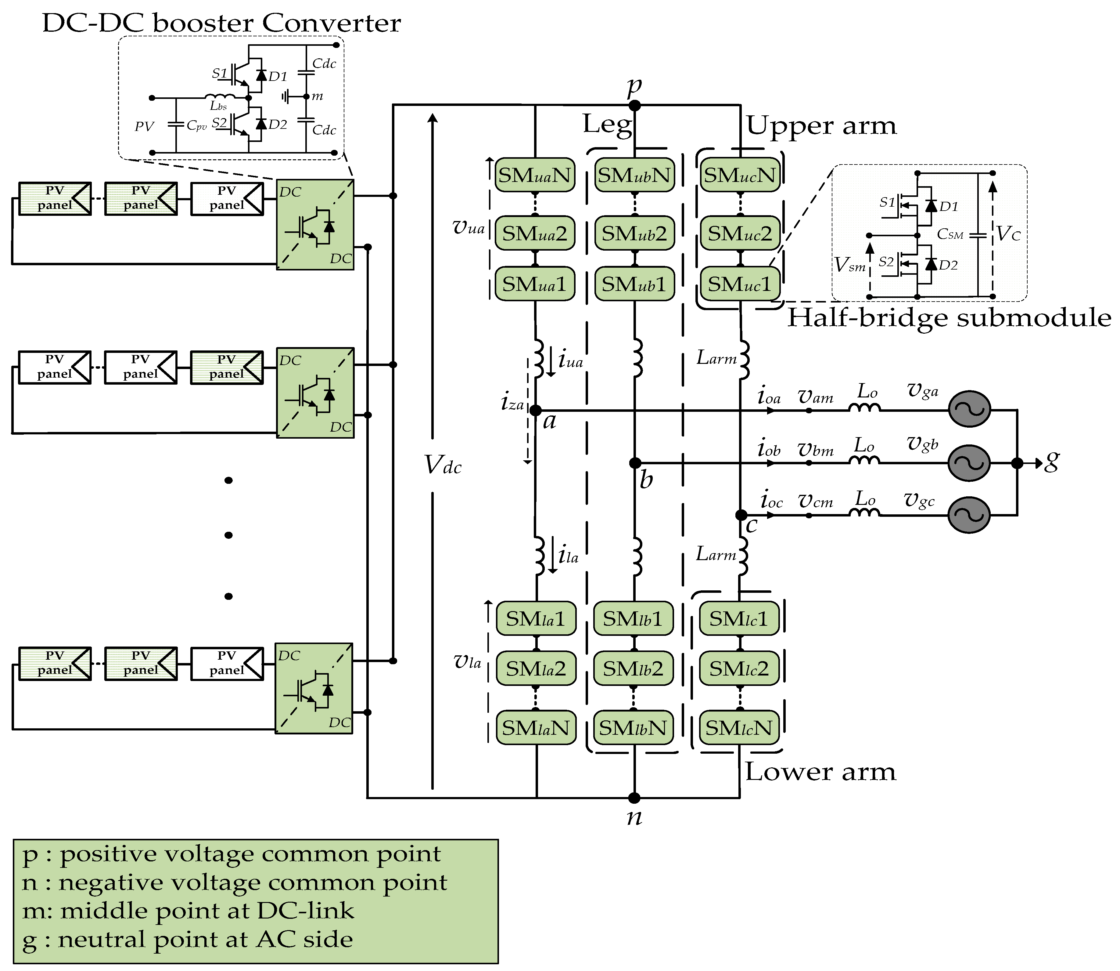
To begin with, a three-phase MMC is linked to an AC grid, as shown in Figure 1, and it is also connected to a number of PV string panels. The MMC controls the required voltage at the DC link, and booster converters are used to step up the voltage and execute the MPPT at each string when a series of PV panels are connected to the DC link.

The MMC has three phase legs; each leg comprises upper and lower arms made up of a number of interconnected SMs. The legs are considered voltage sources since they deliver output voltages from the inserted SM voltages placed into the upper and lower arms, respectively [12,18]. An arm inductor (L_arm) is inserted at each arm in order to reduce and control the circulating currents (i_za, i_zb and i_zc) as well as minimize the DC fault current inside the MMC [12,18].

The SM is normally based on half-bridge and full-bridge topologies, as will be explained. One capacitor, two diodes and MOSFET (or IGBT) transistors make up the half-bridge (HBSM) of the SM topology, whereas two of these components are included in the full-bridge (FBSM) architecture [41,42]. As long as they must work in complementary fashion, each HBSM is inserted when its upper transistor, S1, is in an ON state, and then its lower transistor, S2, is in an OFF state. In this situation, the submodule voltage (V_sm) is added to the arm voltage, and in accordance with the direction of the current, its capacitor will be charged or discharged. Alternatively, the cell voltage is not added to the arm voltage when the SM is bypassed while S1 is in an OFF state and S2 is in an ON state, regardless of the current direction [43,44].

The V_sm may be determined by dividing the DC link voltage (V_dc) by the total number of SMs (N_sm) in the upper (N_u) and lower (N_l) arms in ON states:

$$N_{sm}={N_u+N}_l$$

(1)

$$V_{sm}\cong V_{dc}/N_{sm}$$

(2)

The voltages of the upper and lower arms might be written as (3) and (4), based on Kirchhoff’s voltage law applied to the MMC structure shown in Figure 1. The total voltages of the upper and lower arms in the SMs are v_ux and v_lx, measured as voltages, referring to points p and n, respectively, and the currents in the upper and lower arms are i_ux and i_lx, measured as amperes, where x stands for phases a, b or c:

$$\frac{1}{2}{V}_{dc}-v_{ux}-L_{arm}\frac{{di}_{ux}}{dt}-v_{xm}=0$$

(3)

$$\frac{1}{2}{V}_{dc}-v_{lx}-L_{arm}\frac{{di}_{lx}}{dt}+v_{xm}=0$$

(4)

The output voltage (v_xm) is measured from any phase, x, to the DC middle point, m. Adding (3) and (4) leads to (5):

$$\left(V_{dc}-v_{ux}\right)-v_{lx}=L_{arm}\frac{{di}_{ux}}{dt}+L_{arm} \frac{{di}_{lx}}{dt}$$

(5)

In a similar manner, subtracting (3) and (4) leads to (6) and then to (8) when using the difference between the i_ux and i_lx currents (7) as the output currents (i_ox):

$$v_{lx}-v_{ux}=L_{arm}\frac{{di}_{ux}}{dt}-L_{arm}\frac{{di}_{lx}}{dt}+2v_{xm}$$

(6)

$$i_{ox}=i_{ux}-i_{lx}$$

(7)

$$\frac{v_{lx}-v_{ux}}{2}=v_{xm}+\frac{1}{2}{L}_{arm}\frac{{di}_{ox}}{dt}$$

(8)

Equation (9) represents the output voltage of any phase in relation to the grid voltage, where the output voltage of the grid at each phase referred to as point g is v_gx:

$$v_{xm}=L_o\frac{{di}_{ox}}{dt}+v_{gx}+v_{gm}$$

(9)

The voltage between the AC neutral point, g, and the DC middle point, m, defined as v_gm, could be neglected because there is no returning path for the zero-sequence component of the output currents.

Thus, using the definition of an equivalent inductor (L_eq) at (10), the output voltage (v_ox) can finally be expressed as (11). Equation (11) is typically used to define proportional–integral (PI) controllers to manage the active and reactive powers transferred to the grid.

$$L_{eq}\equiv \frac{1}{2}{L}_{arm}+L_o$$

(10)

$$v_{ox}\equiv \frac{v_{lx}-v_{ux}}{2}\cong L_{eq}\frac{{di}_{ox}}{dt}+v_{gx}$$

(11)

The internal circulating current is arguably a significant variable of the MMC, which may have an important impact on the performance of the MMC as a consequence of its effect on the capacitor voltage ripple and the arm peak current [45]. The DC component of circulating currents typically arises when energy is transmitted from one phase to another or from an external energy source on the DC side to the MMC phases; that energy is transferred to the AC side using the output AC current [46,47].

Furthermore, controllers may be able to transfer energy from the upper arm to the lower arm or back using circulating currents that include a 50 Hz component; this feature is used only when it is required to keep the upper and lower arms balanced. A main concern with the MMC is that a 100 Hz negative-sequence component arises in the circulating current due to the difference in voltage between the upper and lower capacitors [48], and a 100 Hz positive-sequence component or even a zero-sequence component may emerge in unbalanced AC grid configurations. These currents are a source of losses that do not make a real contribution to the MMC, so it is convenient for controllers to reduce them [46,47].

Various types of controllers, including PI and proportional–resonant (PR) controllers, have been proposed to regulate 100 Hz components of the circulating current. These controllers have also been employed to balance power transmission between the phases of the MMC and adjust the DC bus current reference [20,47,49].

Equation (12) defines the circulating current as i_zx at any phase x, and then Equation (13) can be used to describe how the upper arm voltage and the lower arm voltage can be used to control the circulating current:

$$i_{zx}\equiv \frac{i_{ux}+i_{lx}}{2}$$

(12)

$$v_{zx}\equiv \frac{\left(V_{dc}-v_{ux}\right)-v_{lx}}{2}=L_{arm}\frac{{di}_{zx}}{dt}$$

(13)

3. Control Strategy

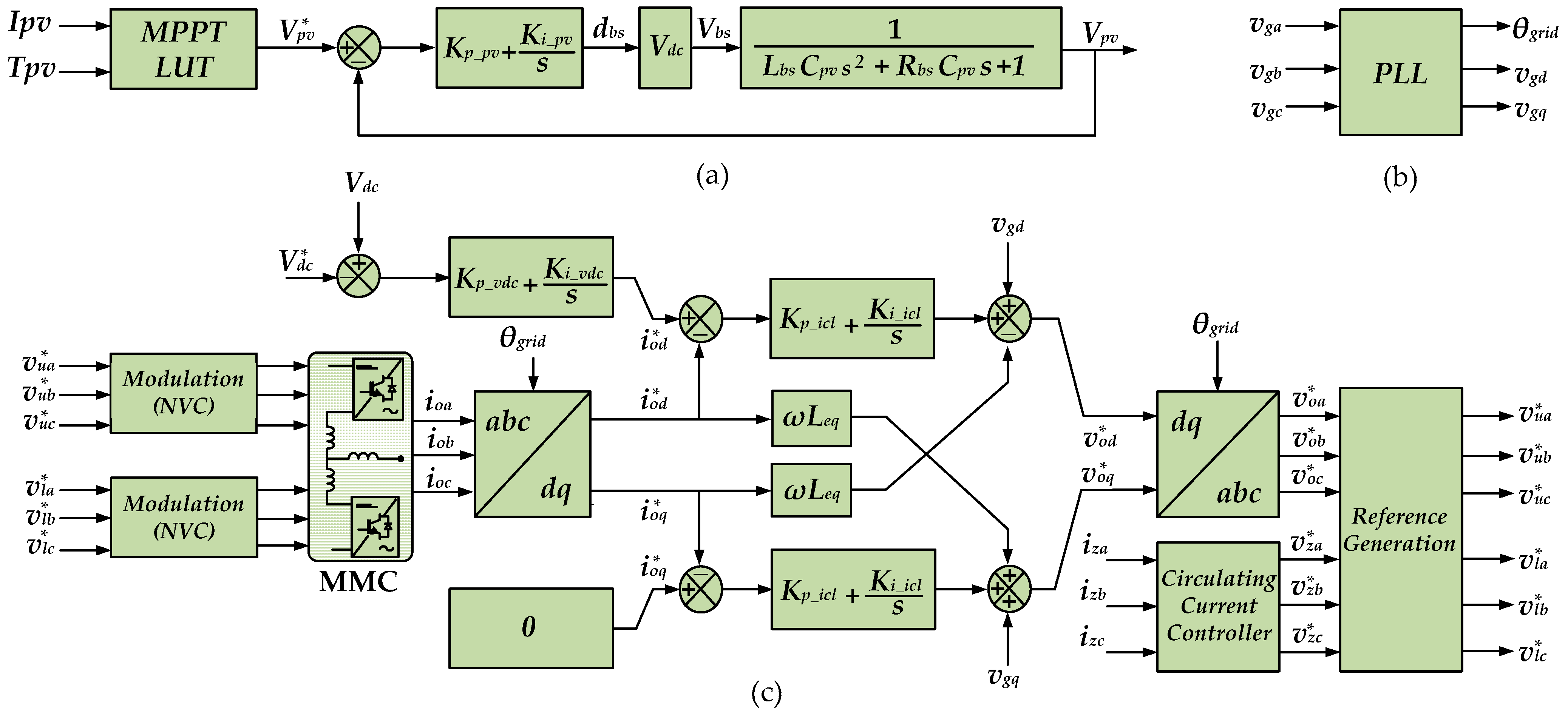
The control of this PV generation application is divided into two parts: first, the series of PV panels are controlled by boosters targeting the maximum power; then, the active power given by the panels is transferred to the grid.

The MPP of a PV series is the combination of voltage and current that supplies the maximum power, and it has a very important role in the performance and efficiency of the PV generation system [9,10]. Any variation in temperature or irradiance must be taken into account when tracking the maximum power point, which therefore must be updated constantly [9]. Because a quick and accurate answer to changes in temperature and solar irradiation is desired, a quite uniform irradiance is supposed, at least for each PV string, and a simple lookup table approach has been employed for the MPPT in this application. The current (I_pv) and the temperature (T_pv) of the PV panels are measured, and then a reference voltage for the PV panels (V*_pv) is read from an LUT that stores the values of voltages at the maximum power point for a large set of currents and temperatures that have been computed offline and can be updated regularly. Then, each PV string is connected to a booster converter, which regulates the voltage of the string following the reference provided by the LUT, giving as much power as possible to the DC input of the MMC. The booster may achieve a large step-up voltage gain to some extent with a large duty cycle on the lower semiconductor [6,7], but small voltage steps are preferred to improve the booster efficiency. Thereafter, a proportional-integral regulator generates the duty cycle (d_bs) of the upper switch at each booster, as described in Figure 2a; actually, to simplify the analysis, the boosters are controlled as choppers, and the voltage of the PV panels is seen as a fraction of V_dc.

The open-loop transfer function used to design the booster regulator is shown in (14), where a constant estimated value of V_dc is used, not a measure. The bandwidth of this transfer function (15) must be smaller than the bandwidth of the two regulators at the AC side in order to make them independent, and, using (17), the PI regulator can be placed at a frequency with a value square root of 3 smaller if a phase margin of 60° is desired.

$$V_{pv}=\left(K_{p\_pv}+\frac{K_{i\_pv}}{s}\right)·{\widehat{V}}_{dc}·\frac{1}{L_{bs}{C}_{pv}{s}^2+R_{bs}{C}_{pv}s+1}(V_{pv}^{*}-V_{pv})$$

(14)

$${BW}_{pv}={\omega }_n=\frac{1}{\sqrt{L_{bs}{C}_{pv}}}$$

(15)

$$\delta =\frac{R_{bs}}{2}\sqrt{\frac{C_{pv}}{L_{bs}}}$$

(16)

$$T_{i\_pv}=\sqrt{3}/{\omega }_n$$

(17)

$$K_{p\_pv}=\sqrt{3}\delta /{\widehat{V}}_{dc}$$

(18)

$$K_{i\_pv}=K_{p\_pv}/T_{i\_pv}$$

(19)

At the AC side, the reference voltages that apply to both the upper and lower arms inside the MMC (v*_ux and v*_lx) are obtained by (20), which is derived from the addition and subtraction of (11) and (13), generating first the output voltage reference (v*_ox) and then the circulating current reduction voltage reference (v*_zx). As described in Figure 2c, the process of controlling v*_ox begins by measuring the three output currents, i_oa, i_ob and i_oc, obtaining the corresponding i_od and i_oq as a result of the synchronization with the grid by a dq frame-based phase-locked loop (PLL) [50,51]. As DC signals, these i_od and i_oq currents are easily managed by using PI regulators; the d component is used to control the active power and regulate the V_dc voltage; meanwhile, the q component reduces the reactive power sent to the grid.

$$\begin{gathered} v_{ux}^{*}=\frac{1}{2}{V}_{dc}-v_{ox}^{*}-v_{zx}^{*} \\ {v}_{lx}^{*}=\frac{1}{2}{V}_{dc}+v_{ox}^{*}-v_{zx}^{*} \end{gathered}$$

(20)

Therefore, the v*_zx values can be used to reduce the circulating currents. As stated above, a PI or a PR can be used to generate them, but a simple proportional controller can also be used, as described in (21). Anyway, for the clarity and repeatability of the results related to the behavior of the proposed NVC method, in this paper, the term v*_zx will be set to zero in most cases and then the 100 Hz circulating current will not be removed.

$$\begin{gathered} v_{za}^{*}=K_{pz}.\left[\left(i_{zb}-i_{za}\right)+\left(i_{zc}-i_{za}\right)\right] \\ {v}_{zb}^{*}=K_{pz}.[\left(i_{zc}-i_{zb}\right)+\left(i_{za}-i_{zb}\right)] \\ {v}_{zc}^{*}=K_{pz}. [\left(i_{za}-i_{zc}\right)+\left(i_{zb}-i_{zc}\right)] \end{gathered}$$

(21)

Regarding AC regulators, it is necessary to control the output currents, and, when using them, the active power and the reactive power, as shown in Figure 2. Following [52], the time constant (Ti_icl) for the output current loop can be found using the time constant of the plant (25), which can be computed by the ratio of the equivalent output reactor, defined in (10), and the series resistance of that equivalent reactor. Therefore, the value of Kp_icl can be found by selecting a bandwidth for the inner loop that is about 5 to 20 times smaller than the switching frequency (22).

$${BW}_{icl}=1/\left({nT}_s\right)$$

(22)

$$K_{p\_icl}=L_{eq}/\left({nT}_s\right)$$

(23)

$$K_{i\_icl}=R_{eq}/\left({nT}_s\right)$$

(24)

$$T_{i\_icl}=L_{eq}/R_{eq}$$

(25)

The outer loop (26) that regulates the active power in order to control the V_dc voltage must be slower than the inner current loop to be decoupled from it; in this case, estimated values for V_dc and v_od are used to compute K_{p_vdc}. Applying the symmetrical optimum [52] and looking for a desired phase margin (ψ), a bandwidth smaller than the previous regulator is chosen using (29) and then the K_{p_vdc} value is finally used to adjust the bandwidth, taking into account that the equivalent capacitance of the MMC corresponds to six parallel arms with N_sm cell capacitors in series (27).

$$V_{dc}=\left(K_{p\_vdc}+\frac{K_{i\_vdc}}{s}\right)·\frac{1}{1+n{T}_{s}s}·\frac{3{\widehat{v}}_{od}}{2{\widehat{V}}_{dc}}·\frac{1}{C_{eq}s}(V_{dc}^{*}-V_{dc})$$

(26)

$$C_{eq}=N_{phases}·N_{arms}·C_{sm}/N_{sm}$$

(27)

$$a=\left[1+sin\left(\psi \right)\right]/cos\left(\psi \right)$$

(28)

$$T_{i\_vdc}=a^2·{nT}_s$$

(29)

$${BW}_{vdc}=1/(a·{nT}_s)$$

(30)

$$K_{p\_vdc}=\left(2{\widehat{V}}_{dc}{C}_{eq}\right)/(3{\widehat{v}}_{od}·a·{nT}_s)$$

(31)

$$K_{i\_vdc}=K_{p_{vdc}}/T_{i\_vdc}$$

(32)

4. Proposed NVC Method

A new algorithm is proposed to implement the NVC technique, in this case for an MMC used in a grid-connected PV generator. Using this method, the converter generates at each sampling period the nearest voltage vector to a given reference. This proposal uses natural coordinates, namely, ab, bc and ca, that help to understand the operations; it is easy to implement in a processor; and it offers a simple paradigm for further developments. In addition, this technique may be used in SVM techniques that look for the nearest vector or the three nearest vectors at their early steps [24,33,34].

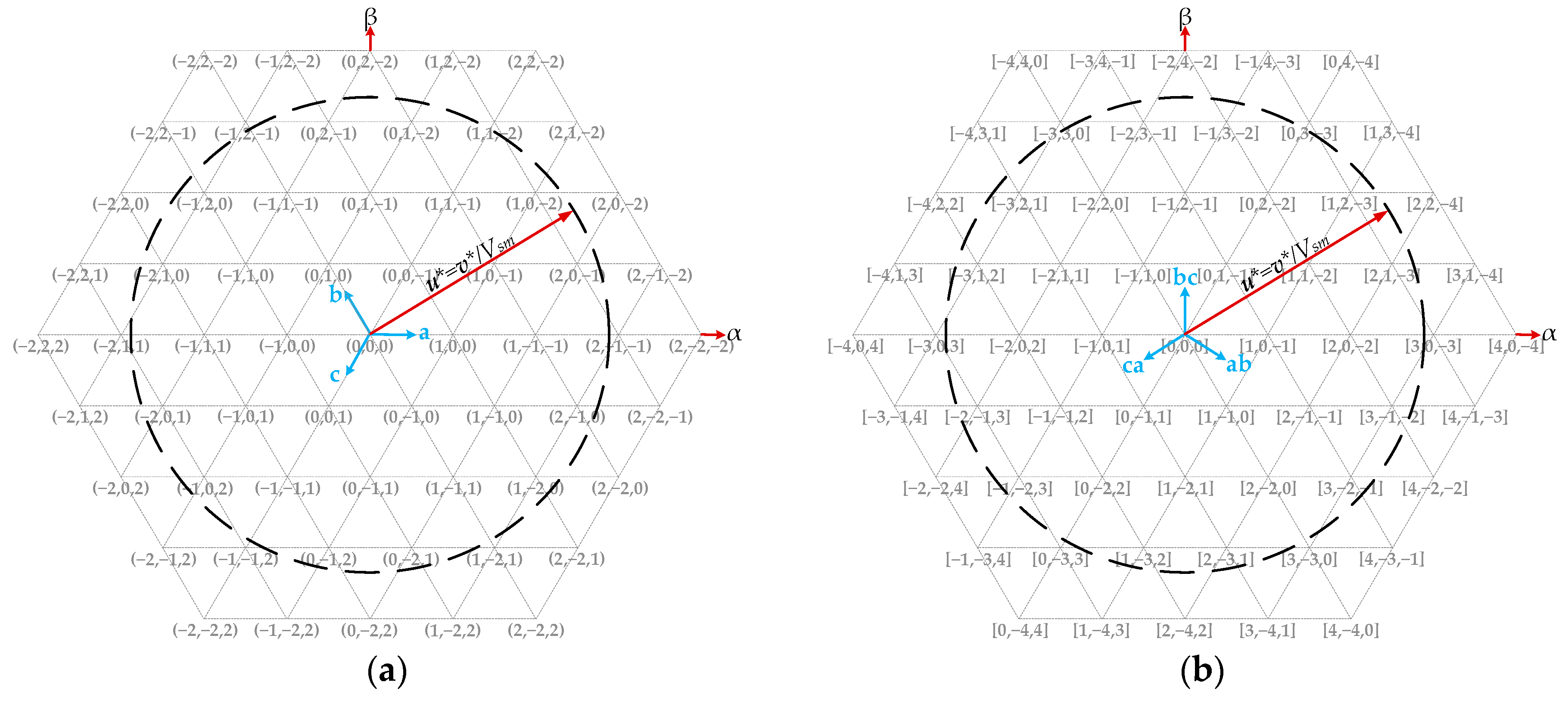
In order to explain this method, an MMC with four SMs per arm is used. In this case, Figure 3 shows the map of the vectors related to the converter states, using phase-to-neutral values in Figure 3a and phase-to-phase values in Figure 3b. It must be noticed that, to differentiate these two types of vectors, curved brackets have been used for the former and square brackets for the latter.

The proposed technique starts by applying a normalization process to a given reference, v* = (v*_a, v*_b, v*_c), that may correspond to the upper arm or to the lower arm, moving to line-to-line values and obtaining a new vector, u* = [u*_ab, u*_bc, u*_ca]. The process usually starts with the lower arm.

$$\begin{gathered} u_a^{*}=v_a^{*}/V_{sm} \\ {u}_b^{*}=v_b^{*}/V_{sm} \\ {u}_c^{*}=v_c^{*}{/V}_{sm} \end{gathered}$$

(33)

$$\begin{gathered} u_{ab}^{*}=u_a^{*}-u_b^{*} \\ {u}_{bc}^{*}=u_b^{*}-u_c^{*} \\ {u}_{ca}^{*}=u_c^{*}-u_a^{*} \end{gathered}$$

(34)

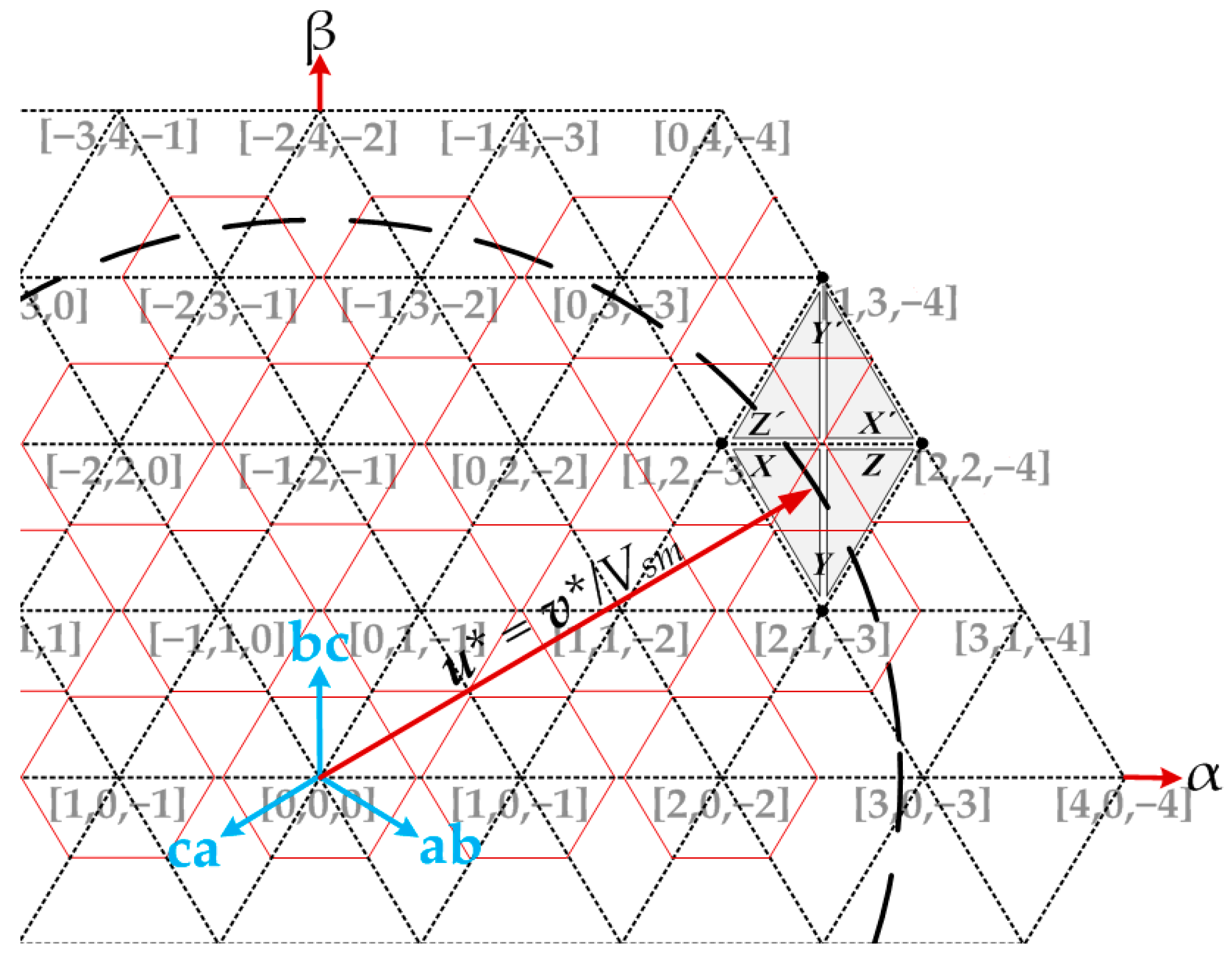
For any reference covered by any of the red hexagons drawn in Figure 4, which means three out of every four situations, the coordinates of the nearest vector are found just by rounding the three normalized values given by (34) to their nearest integers, and the process to find the nearest vector may continue at (50), using η_xy equal to c_xy for xy = {ab, bc, ca}.

$$\begin{gathered} c_{ab}=round\left(u_{ab}^{*}\right) \\ {c}_{bc}=round\left(u_{bc}^{*}\right) \\ {c}_{ca}=round\left(u_{ca}^{*}\right) \end{gathered}$$

(35)

Whenever the rounding of (35) does not lead to a valid vector, because the sum of the three computed coordinates is not zero, it is necessary to locate the vectors X, Y and Z that are the three nearest ones to the given reference, u*. They can be found using (36):

$$\begin{gathered} \mathit{X}={[c}_{ab}–\sigma , c_{bc},c_{ca}] \\ \mathit{Y}={[c}_{ab}, c_{bc}–\sigma ,c_{ca}] \\ \mathit{Z}={[c}_{ab}, c_{bc},c_{ca}–\sigma ] \end{gathered}$$

(36)

where σ is the summation of the three integer coordinates given by (35):

$$\sigma =c_{ab}+c_{bc}+c_{ca}$$

(37)

Actually, as shown in Figure 4, vector X is located near the reference, u*, in the direction of the axis ab, vector Y is the nearest vector moving in the direction of bc, and vector Z can be found in the direction of ca. This is also valid when the three nearest vectors are X’, Y’ and Z’.

In order to find which one of these three vectors is nearest to the reference, it must be known if the reference is located on a “type V” triangle, surrounded by vectors X, Y and Z in Figure 4 and Figure 5a, or if it is located on a “type A” triangle, defined by vectors X’, Y’ and Z’. It must be noticed that, for any of those triangles, vectors X and Z are always located in the same row, so they have the same bc coordinate, but vectors Y and Y’ are located either one row below them on triangles of type “V” or one row above them on triangles of type “A”. Therefore, (38) can be written for triangles of type “V” and (39) can be written for triangles of type “A”:

$$y_{bc}=x_{bc}-1$$

(38)

$$y_{bc}=x_{bc}+1$$

(39)

Applying (36) to (38) and (39), a value of σ = +1 is found for all triangles of type “V” and a value of σ = −1 is found for all triangles type “A”, as shown in Figure 5a. However, a value of σ = 0 can be found when the reference is located inside one of the red hexagons of Figure 4, and then no more operations are required because the nearest vector has been found just using (35).

Afterward, it must be checked if the reference is located in the region “VL” or “VR” of triangles of type “V” (see Figure 5b) or in the region “AR” or “AL” of triangles of type “A”. For the former, references are at the left side of Y if they comply with (40), and therefore the method will choose between vectors X and Y; for the latter, references are at the right side of Y if they comply with (41), and again the method will choose between vectors X’ and Y’:

$$u_{ a}^{*}<y_a$$

(40)

$$u_{ a}^{*}>y_a$$

(41)

Equating (40) and (41) using (36) leads to the same condition in both cases:

$$d_{ab}>d_{ca}$$

(42)

where

$$d_{xy}\equiv \sigma {(c}_{xy}-u_{xy}^{*}) xy=\left\{ab, bc, ca\right\}$$

(43)

Actually, the value of σ has been added to (43) to obtain the same result as in (42) for triangles of type “VL” and triangles of type “AR”, as shown in Figure 5b. If condition (42) is not met, the reference is located on either a triangle of type “VR” or a triangle of type “AL”.

The final step must select the nearest vector, so it must choose X or Y for any reference located on a triangle of type “VL” or “AR”, as seen in Figure 5c, by using coordinates in the axis b. In the case of “VL”, the nearest point is X if condition (44) is met; in the case of “AR”, the nearest point is X if condition (45) is met:

$$u_b^{*}>{(x}_b+y_b)/2=z_b$$

(44)

$$u_b^{*}<{(x}_b+y_b)/2=z_b$$

(45)

Equating (44) and (45) as above, using (36), also leads to the same condition in both cases:

$$d_{ab}>d_{bc}$$

(46)

Whenever the reference is either on a triangle of type “VR” or “AL”, axis c must be used instead of axis b, leading to (47) when the nearest vector is Z; otherwise, the nearest vector is Y:

$$d_{ca}>d_{bc}$$

(47)

Joining (42), (46) and (47), these equations lead to a unique Equation (48) valid for all the cases:

$$\begin{array}{l}if\left(d_{ab}>d_{ca}\right)\\ if \left(d_{ab}>d_{bc}\right) nearest is \mathit{X}\\ else nearest is \mathit{Y}\\ else\\ if\left(d_{ca}>d_{bc}\right) nearest is \mathit{Z}\\ else nearest is \mathit{Y}\end{array}$$

(48)

Therefore, the converter vector nearest to the reference is X when d_ab is greater than d_bc and d_ca, the nearest point is Y when d_bc is greater than d_ab and d_ca, and it is Z when d_ca is greater than d_bc and d_ab. Thus, the following operations give the coordinates [η_ab, η_bc, η_ca] for the nearest vector for all cases:

$$\begin{gathered} if(d_{ab}\ge d_{bc}) \& \left(d_{ab}\ge d_{ca}\right) \\ {\hspace{1em}\hspace{1em}\hspace{1em} \eta }_{ab}=c_{ab}-\sigma ;{\eta }_{bc}=c_{bc}{;\eta }_{ca}={ c}_{ca} \\ if(d_{bc}\ge d_{ca}) \& \left(d_{bc}>d_{ab}\right) \\ \hspace{1em}\hspace{1em}\hspace{1em} {\eta }_{ab}=c_{ab};{ \eta }_{bc}=c_{bc}{-\sigma ; \eta }_{ca}={ c}_{ca} \\ if\left(d_{ca}>d_{ab}\right) \& \left(d_{ca}>d_{bc}\right) \\ {\hspace{1em}\hspace{1em} \eta }_{ab}=c_{ab};{\eta }_{bc}=c_{bc}{;\eta }_{ca}=c_{ca}-\sigma \end{gathered}$$

(49)

An example from Figure 4 has been used to illustrate how this method works in order to offer more clarity. For a reference at phase-to-neutral coordinates, u*_a = 1.60 × V_sm, u*_b = 0.05 × V_sm and u*_c = −1.65 × V_sm, the normalized line-to-line coordinates are [1.55, 1.70, −3.25], obtained by means of (33) and (34).

Rounding by (35) leads to the coordinates [2, 2, −3], giving a value of 1 for σ, using (37). Therefore, the three nearest vectors, based on (36), are X = [1, 2, −3], Y = [2, 1, −3] and Z = [2, 2, −4], and one of them must be chosen.

Then, the three distances d_ab = 0.45, d_bc = 0.30 and d_ca = 0.25 are computed using (43). Since d_ab is greater than d_bc and d_ca, vector X must be chosen as the nearest vector according to (49), and therefore the line-to-line coordinates of the nearest vector are [1, 2, −3], as shown in Figure 3b, which correspond to vector (V_sm, 0, −2V_sm) using phase-to-neutral coordinates, as shown in Figure 3a.

Once the coordinates of the nearest vector have been found, they must be translated into states to determine the number of active cells. Equation (50) applies the method previously proposed in [53] and explained with Figure 6:

$$\begin{gathered} S_{al\_base}=max\left(0, {\eta }_{ab},-{\eta }_{ca}\right) \\ {S}_{bl\_base}=max\left(0, {\eta }_{bc},-{\eta }_{ab}\right) \\ {S}_{cl\_base}=max\left(0, {\eta }_{ca},-{\eta }_{bc}\right) \end{gathered}$$

(50)

Figure 6 shows the base states for phases a, b and c, previously shown in Figure 3b. Figure 6a depicts a map with two sections, one on the right side of the map with values ranging from 1 to N_sm, and the other with a set of zeros. On the right side, phase a involves both coordinates η_ab and negative η_ca; the states should always be positive since the maximum of η_ab is chosen with a negative of η_ca because η_ca is always negative at its crossing with ab, as seen in Equation (50). When coordinate η_ab is negative and η_ca is positive and vectors are on the left side of the map, (50) generates a zero. In addition, phases b and c apply the same ideas using different coordinates.

To give more information, the same example considered above is used. When the normalized line-to-line coordinates are X = [1, 2, −3], applying (50) delivers the state 320; this means that phase a = 3, phase b = 2 and phase c = 0. Considering the complementary behavior of the upper and lower arms, it indicates three active cells in the lower arm and one active cell in the upper arm for phase a, two active cells in the lower arm and two active cells in the upper arm for phase b, and zero active cells in the lower arm and four active cells in the upper arm for phase c.

The next target of this proposed NVC method is to minimize the common-mode voltage, which may result in a better use of the available DC voltage [54,55,56]. The base states given by (50) of the MMC can be modified by means of (54) by using for the three phases the same redundancy value, named ρ [53]. Then, the value of ρ is limited in order to keep the range of active cells between 0 and N_sm because it is not possible to have a negative number of active cells at any arm or more active cells than N_sm. The minimum and maximum values of ρ can be found as follows:

$${\rho }_{max}=N_{sm}-\mathit{max}\left(S_{al\_base},S_{bl\_base},S_{cl\_base}\right)$$

(51)

$${\rho }_{min}=0$$

(52)

Therefore, in order to reduce the common-mode voltage, the value of ρ given by (53) is used to find the minimum average distance of the three phases to the central point given by (N_sm/2, N_sm/2, N_sm/2), constrained by the maximum and minimum values of ρ given by (51) and (52):

$$\rho =round\left(\frac{1}{2}{N}_{sm}-\frac{1}{3}(S_{al\_base}+S_{bl\_base}+S_{cl\_base})\right)$$

(53)

This concept applies to any number of SMs and leads to the value that minimizes the voltage between the AC neutral point and the DC middle point. Applying (53) to the previous example, the state 320 leads to ρ = 0.

Finally, switching states of the lower arms can be obtained by adding the chosen value of ρ to the base states:

$$\begin{gathered} S_{al}=S_{al\_base}+\rho \\ {S}_{bl}=S_{bl\_base}+\rho \\ {S}_{cl}=S_{cl\_base}+\rho \end{gathered}$$

(54)

The upper switching states can be found by applying the same process to the upper arm references, or they can be easily computed as the complement of the lower states whenever the circulating currents are not removed.

$$\begin{gathered} S_{au}=N_{sm}-S_{al} \\ {S}_{bu}={N_{sm}-S}_{bl} \\ {S}_{cu}=N_{sm}-S_{cl} \end{gathered}$$

(55)

The voltages of the capacitors (V_sm) inside the cells must be balanced using a sorting mechanism in order to keep the average voltage of the cells at a particular value. Depending on their voltages and the direction of the arm currents, the SMs with the greatest or the smallest voltages are selected to be inserted or bypassed [21,22].

5. Experimental and Simulation Results

A MATLAB/SIMULINK model was used to verify the performance of the proposed NVC method by simulating a detailed model of an MMC with 16 cells per arm connected to an AC grid. Each one of the 96 cells was simulated using two MOSFET switches with 10 mOhm series resistance and one capacitor per cell. Each string of PV panels, which were composed of 17 serially connected PV panels, as described in

Table 1. Parameters of the Suntech STP320-24/Ve PV panels.

Parameters	Values	Units
Maximum power (Pmax)	320	W
Maximum power voltage (Vmax)	36.7	V
Maximum power current (Imax)	8.72	A
Open-circuit voltage (Voc)	45.6	V
Short-circuit current (Isc)	9.07	A
Diode ideality factor (m)	1.1238	-

, was connected to a booster converter, and 11 strings gave their power to a common capacitor whose voltage was regulated by the MMC. The other parameters of this 60 kW facility are included in

Table 2. Parameters of the three-phase MMC connected to the grid for simulations and experiments.

Parameters	Values	Units
Nominal active power (Pnom)	60	kW
Grid voltage (rms)	400	V
Fundamental frequency (ffund)	50	Hz
Output inductor (Lo)	750	µH
Arm inductor (Larm)	750	µH
SM capacitance (Csm)	40	mF
Number of SM per arm (Nsm)	16	-
SM capacitor voltage (Vsm)	50	V
DC link voltage (Vdc)	800	V
Booster half capacitor at DC link (Cdc)	2	mF
Booster inductor (Lbs)	11	mH
PV string capacitor (Cpv)	4	mF

. A fifth-order polynomial based on the datasheet of the STP320-24-Ve polycrystalline PV module made by Suntech was used to create the PV panel model at standard test conditions (irradiance G = 1000 W/m² and temperature T = 25 °C) [57]. Thereafter, a complete set of polynomials was created with steps of 25 W/m² for irradiance values ranging from 100 W/m² to 1000 W/m² and temperatures from 25 °C to 75 °C with steps of 5 °C.

Regarding the experimental setup, shown in Figure 7, a 16-cell MMC was implemented in a real-time simulator (RTS) called RTbox 240, from accuRTpower.com, using the same parameters that were used in the computer simulation performed using Simulink, but a discrete sampling period of 4 microseconds was used, rather than the discrete 0.25 μs used in MATLAB/SIMULINK. The controller was implemented on a 128-MFLOP floating-point processor synthesized on an external Xilinx LX150 Spartan-6 FPGA, and the plant, including the PV panels, a booster, the MMC and a three-phase grid, ran on the RTS using a 4-GFLOPS vectorial processor. The sampling period for the controller that executed the PV panel control, grid synchronization, power regulation and then applied the NVC technique was 20 μs. Meanwhile, the plant was composed of an averaged model of each arm of the MMC, the grid connection filters and the power grid; they were implemented in the RTbox system. The external control of the MMC was achieved by means of a Spartan-6 FPGA module together with a breakout board with many 12-bit ADC and DAC converters that allow the exchange of analog signals in the range from 0 V to 3 V; in this case, the grid currents, the grid voltages and the DC voltage were sent to the external controller; the 96 MMC cell voltages were not exchanged as long as only 6 averaged cell voltages were computed, one for each MMC arm. The control of the booster that applied the MPPT was implemented on a secondary floating-point processor inside the RTbox with a sampling period of 200 microseconds. The C programming language was used for all controllers, including floating-point variables and vectors.

At the AC side, the time constant for the output current loop, Ti_icl, was found using the time constant of the plant (25), as stated above. The value of the reactor resistance is difficult to assess, and it will change with temperature, but an estimated value of 20 ms can be selected. The value of Kp_icl can be found by selecting a bandwidth for the inner loop that is about 5 to 20 times smaller than the switching frequency (22). In this case, the switching frequency of the NVC-controlled MMC was not constant, but it was estimated to be near 1.5 kHz, so a bandwidth of 133 Hz was selected for the internal current loop, and this regulator was applied with a sampling period (T_S) of 20 μs. A bandwidth of 35 Hz and a phase margin (ψ) of 60° were chosen for the outer loop that regulates the active power in order to control the V_dc voltage using (26); it was clearly slower than the inner current loop. At the DC side, the booster regulator generated the duty cycle of the converter every 200 μs. The bandwidth was selected at 24 Hz, smaller than the other two regulators, and in order to obtain a phase margin of 60°, the PI regulator was located at a frequency √3 smaller than the bandwidth set by the booster reactor and the PV panel capacitor (17). These decisions led to the coefficients for the PI controllers shown in

Table 3. The proportional and integral coefficients for the PI controllers.

PI Regulator	Ti	Kp	Ki	Bandwidth
MMC output current control	20 ms	1.88 V/A	93.75 V/A·s	133 Hz
Grid active power control	8.4 ms	11.0 A/V	1315 A/V·s	35 Hz
PV string voltage control	11.5 ms	0.00067 V−1	0.059 V−1·s−1	24 Hz

.

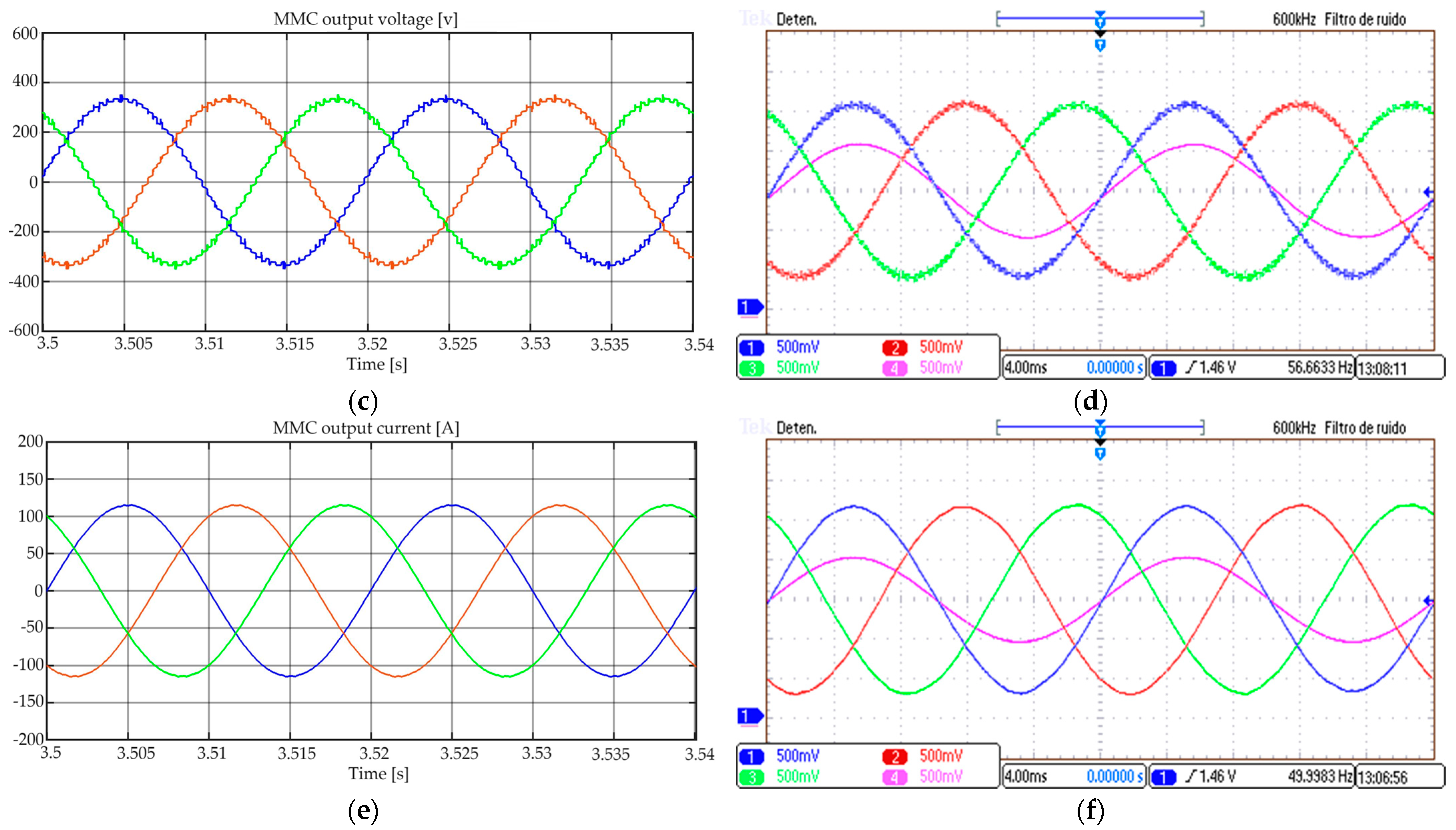
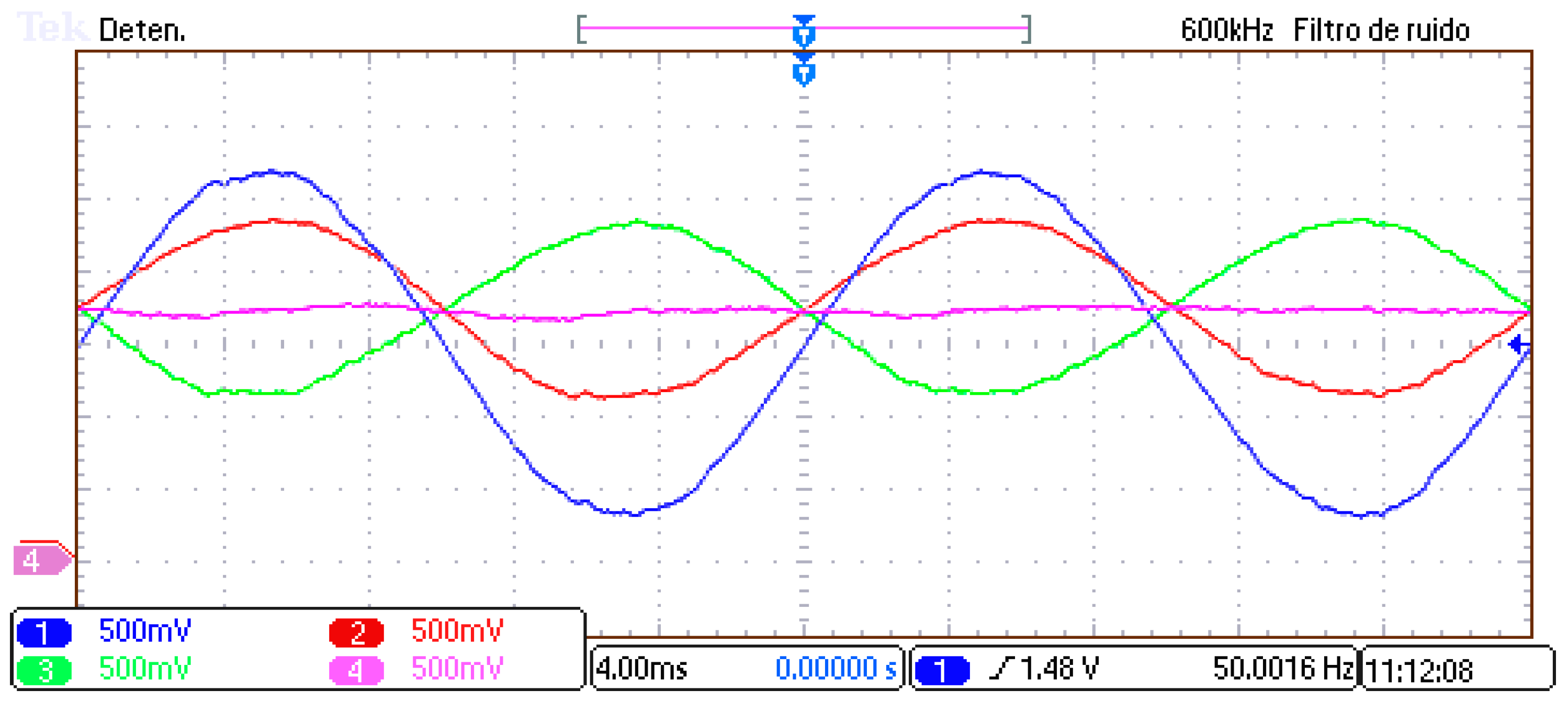
Figure 8 shows the results of the suggested NVC approach in both simulations and experiments. At the grid and the MMC, the proposed NVC output waveforms are mostly sinusoidal. The number of switchings at the peaks and valleys of the MMC output voltage increases a bit, which improves the quality of the current at the grid. 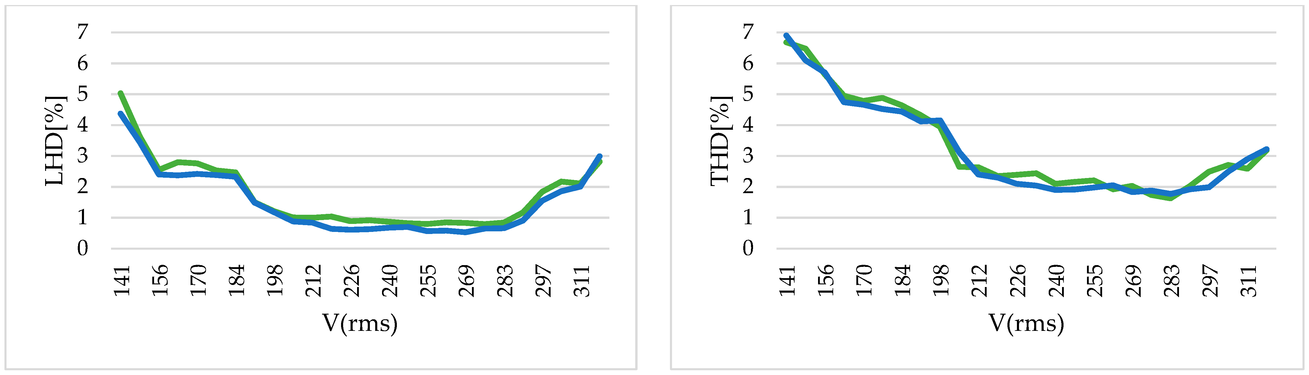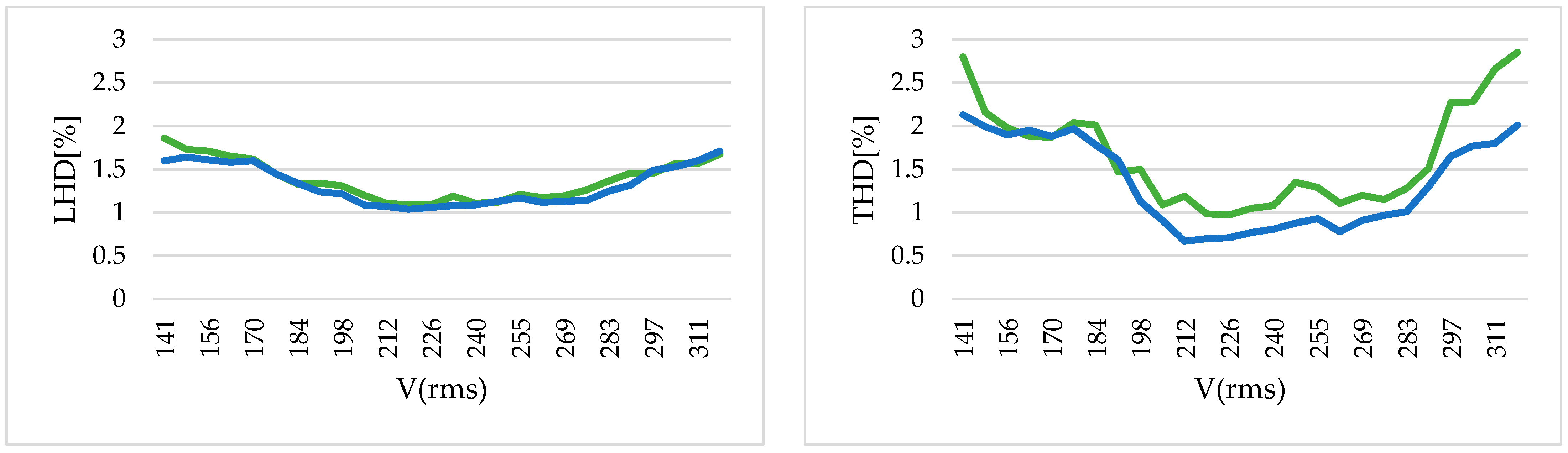The experimental waveforms of the proposed NVC method are shown in Figure 8b,d,f, and they are consistent with the behavior of the simulation using Matlab, shown in Figure 8a–c. This correspondence can also be confirmed by the values obtained by measuring the THD and the low-order harmonic distortion (LHD), up to the 20th harmonic, with fixed 100% irradiance and 25 °C in a steady state, as illustrated in Figure 9 and Figure 10; these measures were taken after a few seconds from the startup using a strong low-pass filter for the measured values. However, there were a few differences: in general, distortions of NVC in the Matlab simulations were smaller than in real time, most probably because many more errors were present in the experiments. Actually, and starting with the most relevant issue, the sampling period for the plant was 4 μs in the real-time model, mainly because of the computational load of the MMC, and first order integrators were used, but the Matlab model used four order integrators and a sampling period of 0.25 μs; the quantization and conversion errors were also present in the 12-bit analog signals transmitted during the experiments; the precision of the floating point of the real-time system was also smaller than the double precision used by Matlab, using only 35 bits for mantissas; finally, but also important for their effect on regulators, delays from the measures at the plant to the actions at the controller were present in the experiments, but they were ignored in the computer simulations.

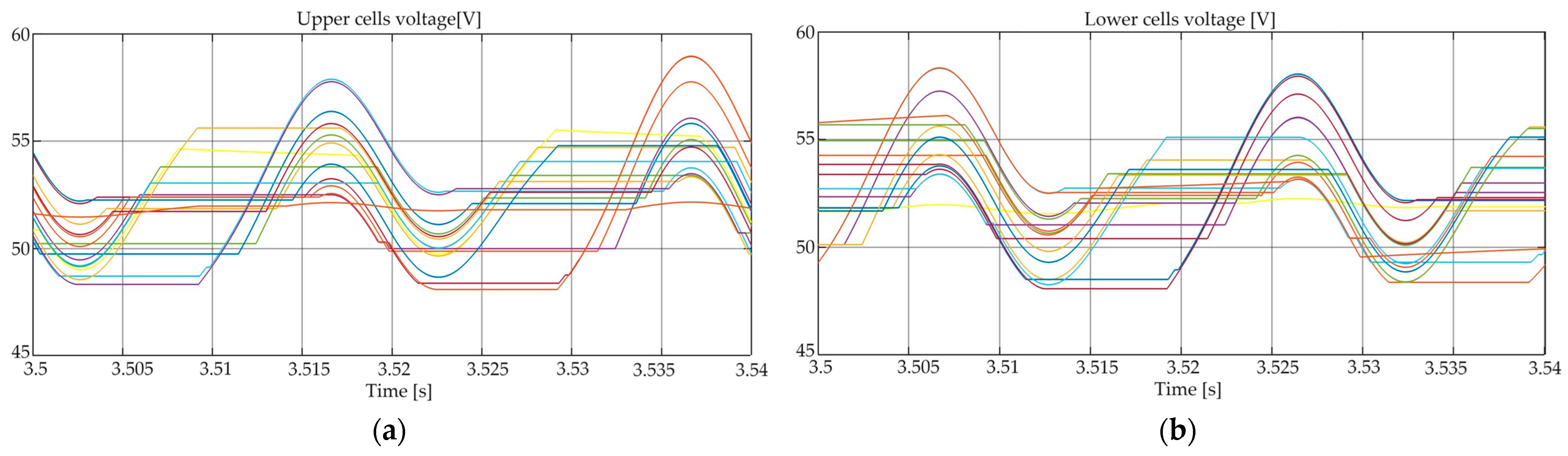
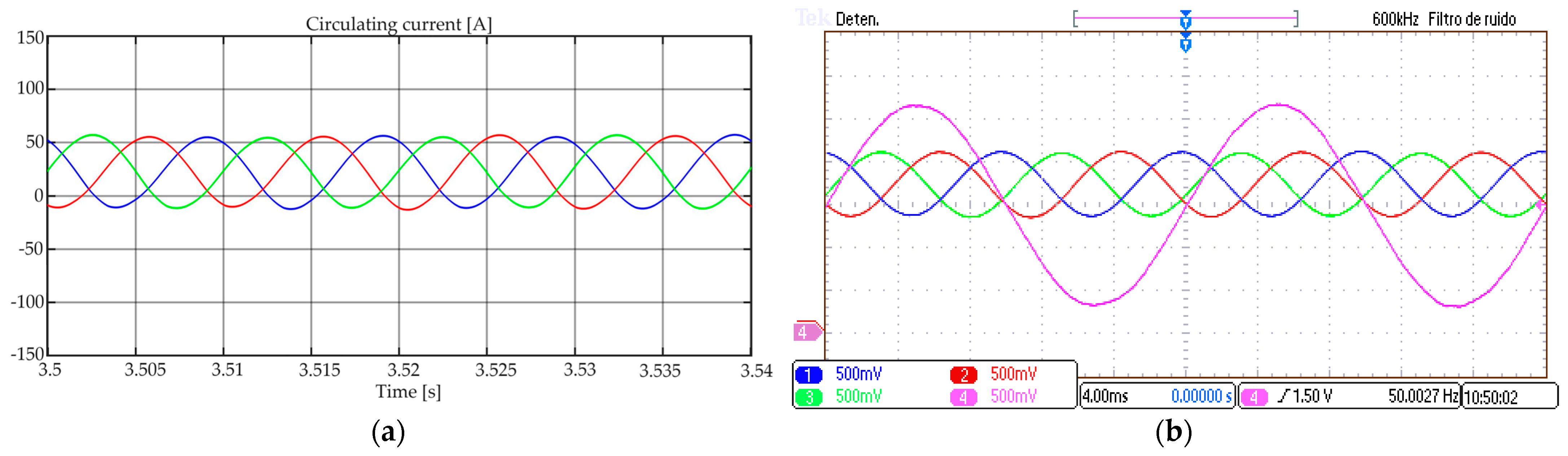
Figure 11 shows that the simulation of the proposed NVC approach generates SM capacitor voltages that are near the target value of 50 V, with a fluctuation of roughly 4 V on average; also, in the experimental setup, the SM capacitor voltages have a similar behavior. Additionally, the MMC circulating currents in the Matlab simulation and the experimental setup are shown in Figure 12. These currents have, as expected, a DC component of nearly 25 A, which corresponds to one-third of the total DC current, and a second-order harmonic component (100 Hz) with a negative sequence.

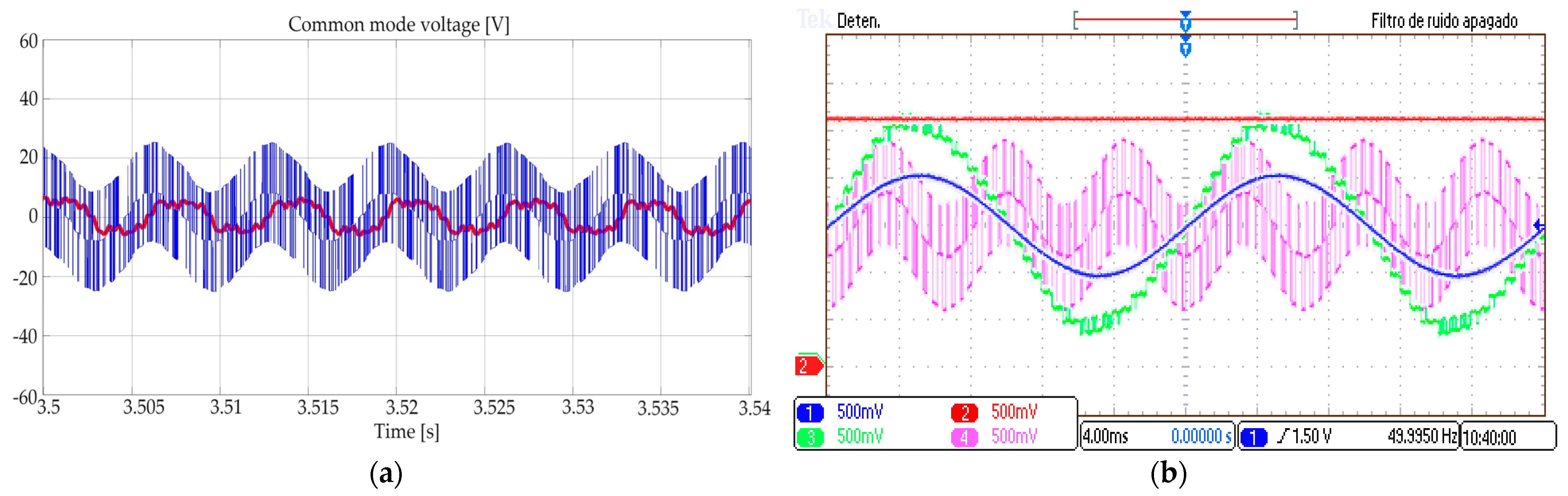
The voltage from the DC middle point to the AC neutral was kept low in both the simulation and experiments, as displayed in Figure 13. The proposed NVC technique tries to reduce the common-mode voltage, and it has been registered that this was about (+5, −5) V in the simulation and about (+10, −10) V in the experimental setup; most probably, the difference is due to the higher sampling period: 4 μs in the experimental setup and 0.25 μs in the simulation.

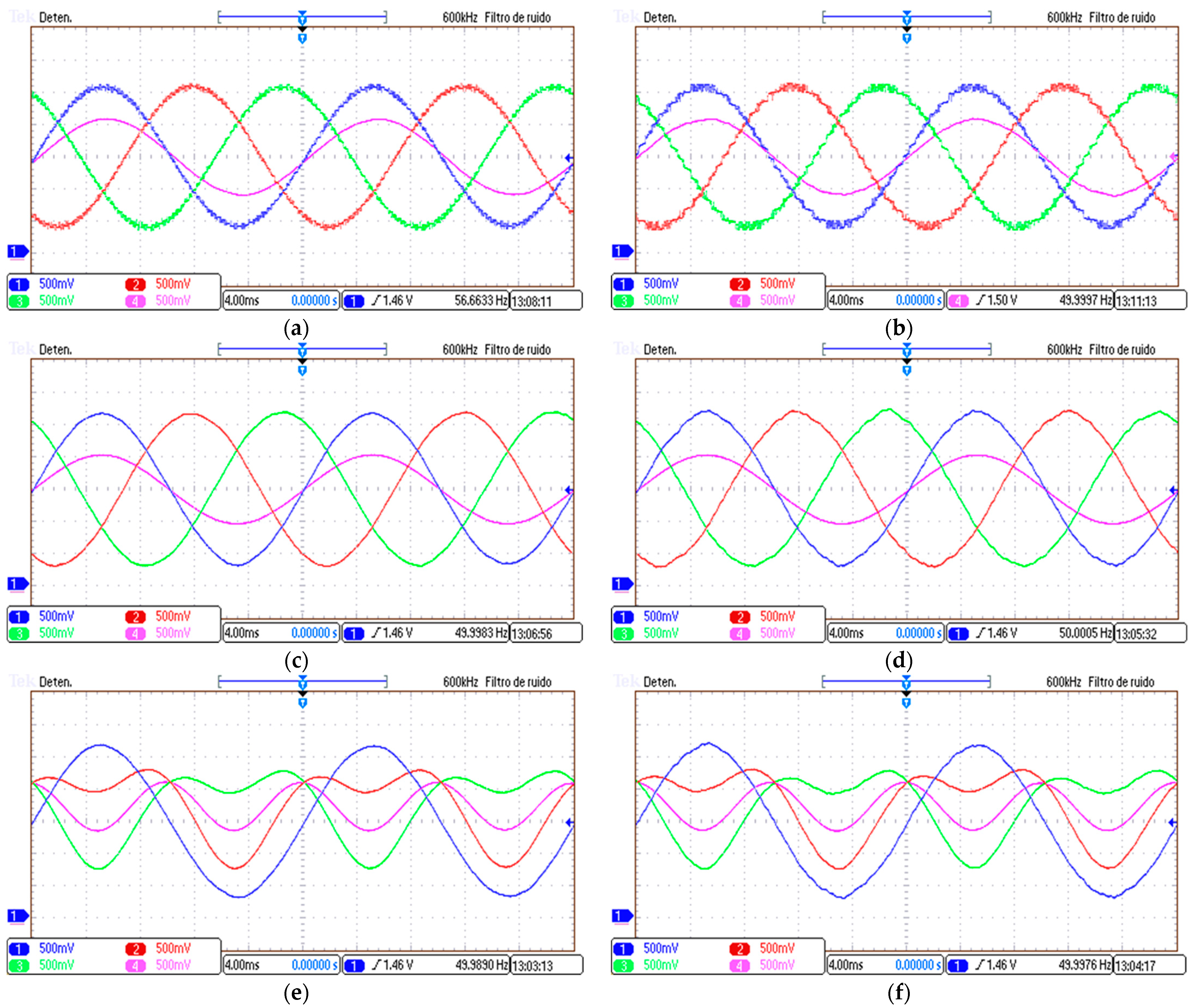
For comparison between the proposed NVC technique and the conventional NLC, the techniques were applied in the experimental setup under identical conditions. From the following figures, it is clear that the NLC produces more distortion than the NVC with respect to both the grid currents and the MMC voltages, particularly at the peaks and valleys. The experimental waveforms of the proposed NVC method and the NLC approach are shown in Figure 14a–f.

As can be seen, the proposed NVC output waveforms are primarily sinusoidal. Also, the output currents were almost pure sinusoidal signals in the NVC, but a quantization issue occurs at the peaks and valleys when using the NLC, which causes a clear distortion, as illustrated in Figure 14d,f; it is clear that, depending on the modulation index, the NLC is unable to choose a good timing for switchings at peaks and valleys. In contrast, these quantization issues in the NLC are not relevant in the NVC, as shown in Figure 14d,e. As a result, the NLC has a greater value for THD and LHD than the proposed NVC technique, as registered in Figure 15 and Figure 16. Overall, it can be said that the NVC has superior control over the output voltage of the MMC and also over the output current quality.

Meanwhile, the circulating currents of the MMC, when the appropriate controller was not applied, were dominated, as expected, by a DC component and a second-order harmonic component, with the same behavior for both the NVC and NLC methods, as shown in Figure 14e,f.

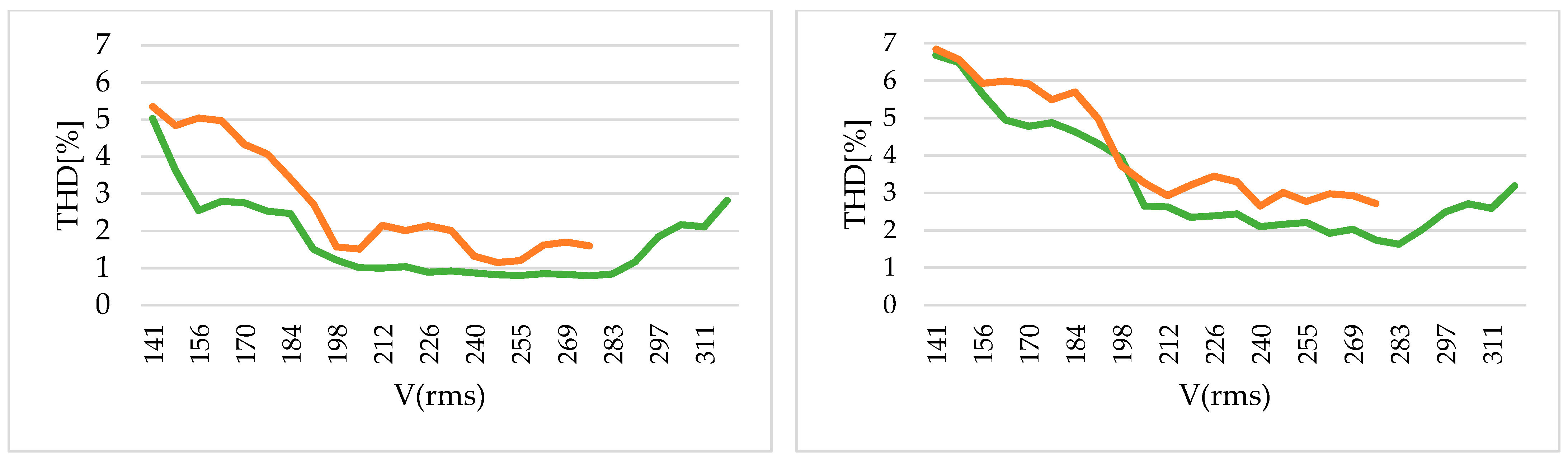
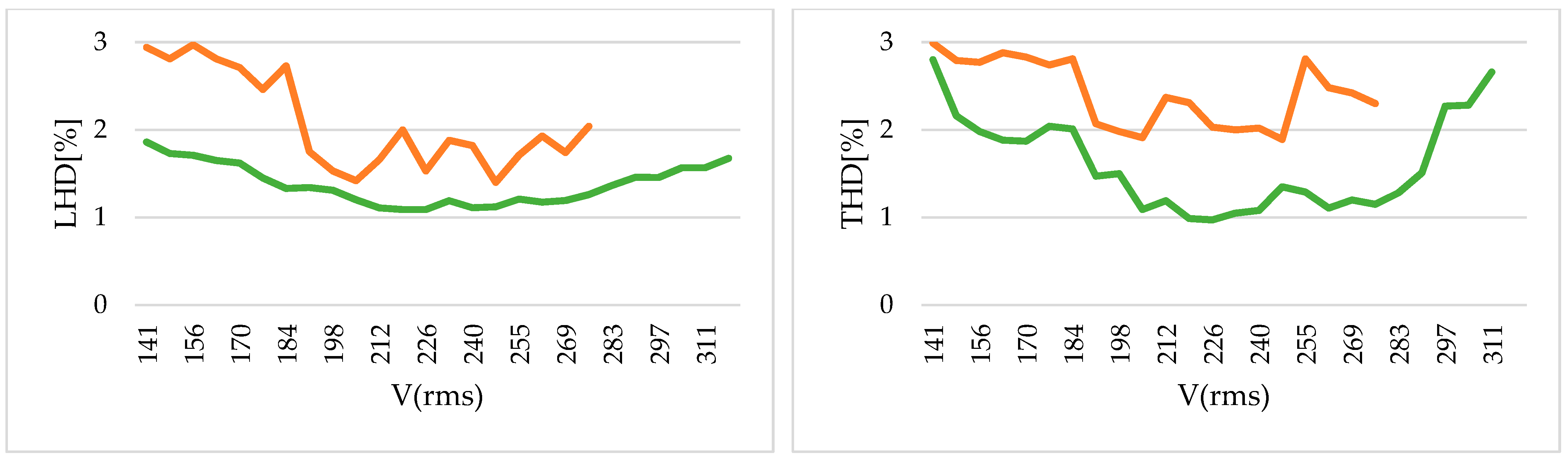
Figure 15 and Figure 16 demonstrate the clear advantage of NVC when it is compared to NLC: the low-order distortion produced by NVC is not only smaller, but also much more consistent and more insensitive to variations in the modulation index (M), while NLC exhibits a more uneven and irregular behavior for equivalent variations in the grid voltage. In addition, as is widely known, it is also evident that the NVC can work with M values of up to nearly 1.15. For instance, when M = 1.12, the distortion of the MMC and the grid is still acceptable when using NVC, but the maximum acceptable results for the NLC modulation are around M = 0.975. The reason for these different behaviors is well known: in the case of NVC, the variations in the common-mode voltage help to reach a higher modulation index [30,32]. In both cases, the DC middle point and the AC neutral point are not connected, but NVC uses line-to-line voltages while NLC uses phase-to-neutral voltages with no zero-sequence injection.

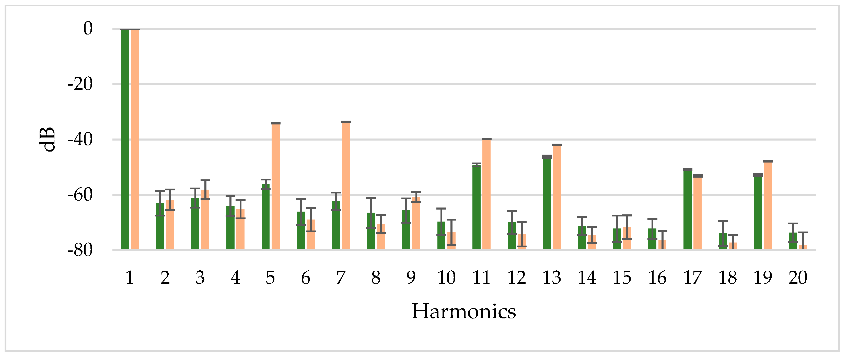
For greater detail, Figure 17 illustrates the behavior of low-order harmonics generated by the MMC at the output currents by the NLC modulation and the proposed NVC technique. Values given in Figure 17 are the average of 20 rounds of measures captured 10 s after the startup at the three phases. The most relevant harmonics are those that are multiple of six plus one and minus one (the 5th and 7th, the 11th and 13th, and the 17th and 19th); the others are mostly below −60 dB. Focusing on these harmonics, the behavior of NVC and NLC modulations is very consistent, as demonstrated by the low values of the standard deviations shown in Figure 17. Furthermore, compared to NLC, the proposed NVC technique achieved an average reduction of 11.2 dB for these harmonics, with a computed standard deviation of 0.76 dB. Most importantly, it has obtained a clear and consistent reduction of about 25 dB in the fifth and the seventh harmonics.

The ability to remove the circulating currents when using the proposed NVC technique is shown in Figure 18 and Figure 19, where the proportional controller described by (21) was applied during half a second. The 100 Hz component of the circulating current was reduced by about 85%, from roughly 27 A (rms) to about 4 A (rms), when using a value of K_pz near 1 V/A, and therefore the impact on the losses of the reduced circulating currents became mostly irrelevant. Figure 19 shows a detailed view of the resulting waveforms.

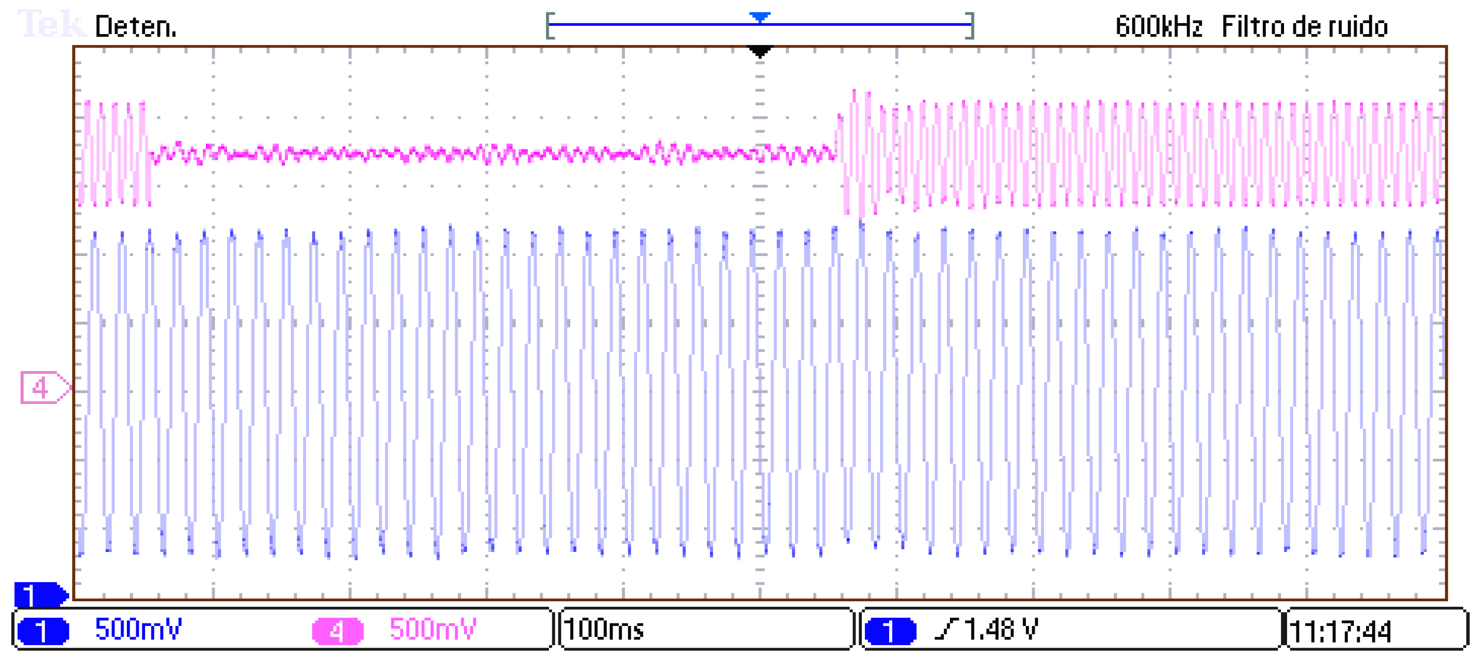
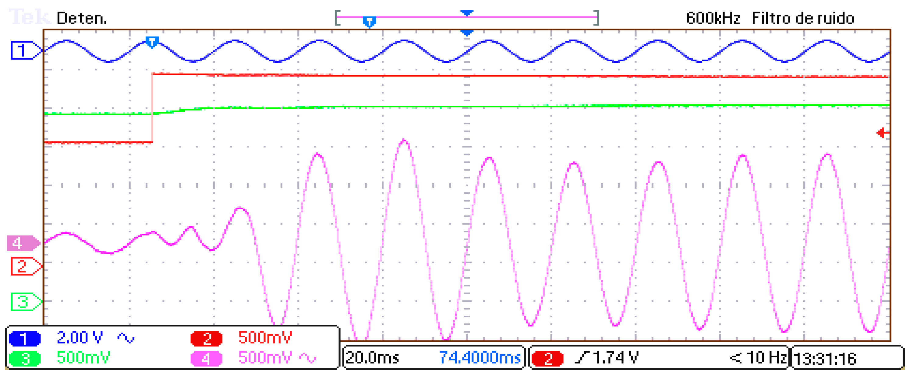
Finally, Figure 20 shows the fast response of the MMC when irradiance changes sharply from 10% to 100%. The quick response is the result of using an LUT for tracking the MMP in the PV panels, and it demonstrates the robustness of the proposed NVC approach for this application.

6. Conclusions

This paper has presented new and straightforward equations for the NVC technique applied in an MMC for a grid-connected PV system, which are applicable at any number of levels. Compared to the scalar NLC technique, which generates three independent states for the three phases, the line-to-line oriented NVC method offers a more coordinated behavior for three-wire converters, as can be seen in the reported reduction in distortion in the low-order harmonics in the output current, mainly in the fifth and the seventh harmonics, and it has been demonstrated that it is clearly more insensitive to changes in the modulation index. The method thoroughly described in this paper depends on the natural coordinates ab, bc and ca; the resulting equations are valid for all converter levels; and their use is very straightforward. As reported, the proposed method is independent of artificial coordinate transformations and lookup tables, which eases further developments. Additionally, converter redundancy states have been used to reduce the common-mode voltage, which may lead to improved utilization of the available DC voltage. The proposed method has provided high-quality voltage and current waveforms with low distortion in both THD and LHD. It delivers a very robust response to quick changes in irradiance, allowing very fast MPPT techniques. An experimental setup for a three-phase MMC connected to a grid with 16 SMs in each arm and a simulation model have been used to validate the new equations that have been proposed for this technique.