An Advanced Explainable Belief Rule-Based Framework to Predict the Energy Consumption of Buildings

Abstract

The prediction of building energy consumption is beneficial to utility companies, users, and facility managers to reduce energy waste. However, due to various drawbacks of prediction algorithms, such as, non-transparent output, ad hoc explanation by post hoc tools, low accuracy, and the inability to deal with data uncertainties, such prediction has limited applicability in this domain. As a result, domain knowledge-based explainability with high accuracy is critical for making energy predictions trustworthy. Motivated by this, we propose an advanced explainable Belief Rule-Based Expert System (eBRBES) with domain knowledge-based explanations for the accurate prediction of energy consumption. We optimize BRBES’s parameters and structure to improve prediction accuracy while dealing with data uncertainties using its inference engine. To predict energy consumption, we take into account floor area, daylight, indoor occupancy, and building heating method. We also describe how a counterfactual output on energy consumption could have been achieved. Furthermore, we propose a novel Belief Rule-Based adaptive Balance Determination (BRBaBD) algorithm for determining the optimal balance between explainability and accuracy. To validate the proposed eBRBES framework, a case study based on Skellefteå, Sweden, is used. BRBaBD results show that our proposed eBRBES framework outperforms state-of-the-art machine learning algorithms in terms of optimal balance between explainability and accuracy by 85.08%.

1. Introduction

The energy consumption of buildings plays a significant role in climate change [1]. The construction industry is responsible for around 40% of global energy consumption [2]. Moreover, rapid population growth has increased the energy demand for buildings [3]. Hence, buildings need to be energy efficient and one effective way to realize this goal is predictive analytics of buildings’ energy consumption [4]. Such predictive consumption is beneficial to utility companies, users, and facility managers to understand a building’s energy performance, and improve its energy efficiency [5]. An efficient use of energy increases monetary savings and improves energy security [6]. The energy prediction of buildings also supports policymakers to implement urban greening policy [7].

Predictions can be computed with both a data-driven approach and knowledge-driven approach [8]. A data-driven approach extracts actionable insight from data. Machine learning, a data-driven approach, builds a statistical model of training data [9]. However, it lacks feature vector to process natural raw data directly [10]. Deep learning based on neural network architecture applies a representation-learning method to extract hidden features from pre-processed raw data [11]. On the other hand, a knowledge-driven approach represents human knowledge in the form of rules [12]. It is constituted by an expert system, which has two components: a knowledge base and inference engine. Belief Rule-Based Expert System (BRBES), fuzzy logic, and MYCIN [13] are examples of knowledge-driven approaches. However, wrong or blank input data, caused by human error or ignorance, can make the predictive output inaccurate, leading to uncertainties [14]. A vagueness of human knowledge and imprecision or incompleteness due to the limit of human knowledge cause such uncertainties [15,16]. Therefore, these uncertainties have to be processed properly. The rule base of BRBES is based on a belief structure, which is known as belief rule base. This belief rule base can capture uncertainty and nonlinear causal relationships [17]. Moreover, BRBES updates belief degrees of the rule base if any or all of the input data become unavailable [18]. The BRBES infers useful conclusions from the rules using the Evidential Reasoning (ER) approach [19,20]. Thus, to deal with uncertainties, especially those caused by ignorance due to input data unavailability, the BRBES outperforms other knowledge-driven approaches [18].

Data-driven machine learning and deep learning models offer high predictive accuracy in exchange for complex mathematical functions [21]. The decision-making process of such models is opaque due to their complex structure. However, when the prediction of the buildings’ energy consumption impacts the policymakers’ decisions, they must know the prediction’s rationale [22]. Therefore, transparency in predicting energy consumption is crucial [23]. A transparent prediction model explains the reasons of its output, resulting in trust relationship between the model and the user. To build this trust, explainable artificial intelligence (XAI) is useful. XAI models are divided into two groups: (a) post hoc explainability and (b) transparent models [24]. The post hoc (after the event) technique is a proxy explanation, which does not consider knowledge or facts of the concerned application area. This explanation is dependent on training data. If the training dataset is biased or erroneous, the post hoc explanation will become misleading. On the other hand, predictive outputs of transparent models are explainable because they have a simple structure. However, the transparent models have low accuracy. Explanation based on knowledge or facts of the concerned application area, instead of training data, is more trustworthy to a human user. Building owners are also more likely to trust a predictive output, which is explained by knowledge or facts related to the energy consumption area. Hence, this study employs a BRBES, an inherently transparent rule-based model, to predict and explain the energy consumption of building based on relevant domain knowledge. Here, ‘domain’ means the application area, which is the ‘energy consumption of building’ in this study. ‘Knowledge’ is represented by rules in the rule base of BRBES. Thus, the rule base of the BRBES represents the knowledge of the energy consumption domain. Facts of this domain are captured with the rule base [17]. As a transparent model, the BRBES has higher explainability and lower accuracy compared with the opaque AI models, but to address this trade-off, we jointly optimize both the parameters and structure of the explainable BRBES using the Joint Optimization of Parameter and Structure (JOPS) [25] to improve accuracy. We propose an explanation interface after the predictive output of the optimized BRBES. We explain the prediction to the user in non-technical human language through this interface. An optimal balance between explainability and accuracy is critical for an XAI model to achieve accurate output and explain the rationale behind it. Therefore, we propose Belief Rule-Based adaptive Balance Determination (BRBaBD) to evaluate the balance of our proposed model between explainability and accuracy. Thus, our proposed advanced explainable BRBES (eBRBES) framework aims to develop a prediction model with optimal balance between explainability and accuracy. This eBRBES framework outperforms the post hoc explanation of black-box machine learning models by dealing with data uncertainties and producing human-understandable explanations based on domain knowledge. To realize our objective, we address the following research questions in this paper:

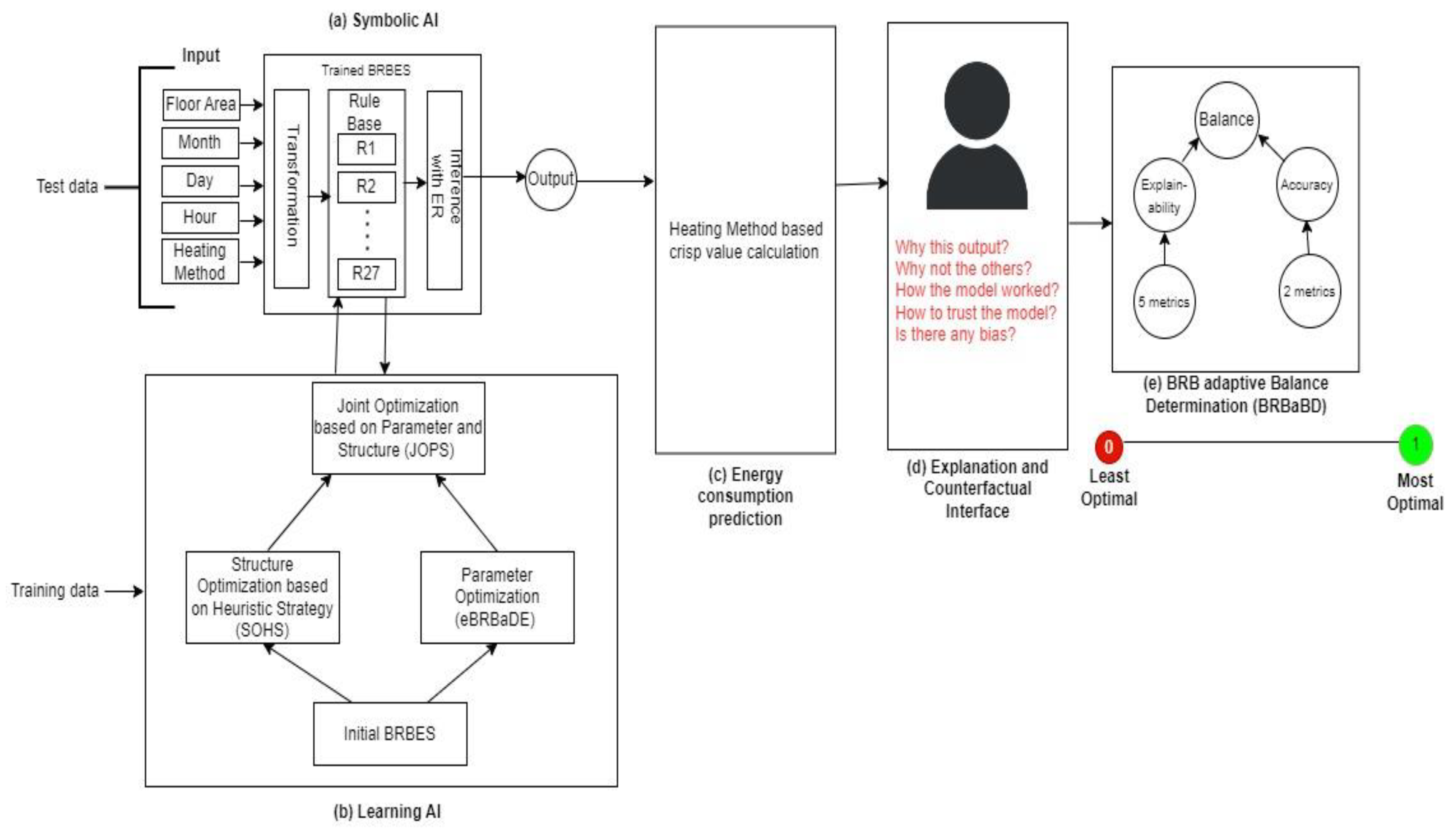
• What is the benefit of applying the BRBES? The key benefit is the domain knowledge-based transparent prediction, while handling data uncertainties.
• How to explain the output of the BRBES? We consider the most important rule of the rule base and building heating method to explain the output via explanation interface.
• How to improve the accuracy of the BRBES? We apply JOPS on the BRBES to improve its accuracy.
• How to address the explainability versus accuracy trade-off? We propose BRBaBD for this purpose.

Furthermore, we generate a counterfactual statement against the explanation to enable the user to understand why another output did not occur. Thus, we make our proposed model trustworthy to the building owner.

2. Related Work

Zhang et al. [26] proposed explanation modules for a Random Forest (RF)-based building energy model. They used a Partial Dependence Plot to explain the feature importance. They interpreted local space with decision tree surrogates, which do not consider domain knowledge. Moreover, RF is a data-driven approach, which does not address data uncertainties. Tsoka et al. [27] employed an Artificial Neural Network (ANN) to classify the Energy Performance Certificate of a building. They used XAI tools Local Interpretable Model-agnostic Explanations (LIMEs) and Shapley Additive Explanations (SHAP) to identify the most influential input features for the ANN. However, the ANN is a black-box model without any domain knowledge. LIMEs’ local explanation and SHAP’s feature importance are proxy. Moreover, an ANN does not address data uncertainties. Miller [28] investigated what types of behaviors are the most important in the context of the primary use-type of a building and its energy consumption level. A Highly Comparative Time-Series Analysis (HCTSA) toolkit was used to analyze the most important temporal features of energy meter data to classify building performance. HCTSA uses Support Vector Machine (SVM), with linear kernel, to classify temporal features extracted from the time-series data of the energy meter. However, SVM does not deal with data uncertainties. Moreover, HCTSA does not consider domain knowledge. Fan et al. [29] proposed a new LIME-based methodology to explain and evaluate five supervised building energy performance models. They also developed a novel evaluation metric, trust, to quantitatively evaluate each prediction based on evidence type. However, a LIME-based local explanation is ad hoc. Such explanation is based on the training dataset only, without any consideration of domain knowledge.

Zhang et al. [30] used Light Gradient Boosting Machine (LightGBM) integrated with SHAP to predict energy consumption of buildings. However, LightGBM is not inherently transparent. As a post hoc tool, SHAP gives a proxy explanation. Moreover, it does not consider domain knowledge and data uncertainties. Li et al. [31] proposed a Prediction–Explanation Network (PEN) to predict stock price movement with better explainability. They employed a shared representation learning module to identify the correlation between text and stock price with a vector of salience. However, this PEN framework is based on a recurrent neural network, which does not use domain knowledge. Data uncertainties are also not dealt with by this PEN framework. Yu et al. [32] showed how background knowledge, extracted with rule induction techniques, can be applied to give succinct formal explanations. However, this background knowledge is represented by traditional if–then rules and a boosted tree, which cannot deal with uncertainties. Müller et al. [33] proposed a combined approach of inductive logic programming and a Convolutional Neural Network (CNN) to detect defects as part of industrial quality control. However, a CNN does not deal with domain knowledge, and inductive logic programming does not address uncertainties. Hence, this method does not have full-fledged domain knowledge-based explainability. Chung et al. [34] employed a deep learning model to predict the energy demand of office buildings. They used the XAI technique SHAP to identify essential input parameters for this deep learning model. They demonstrated that these input parameters vary with localized climate. However, deep learning, being a data-driven approach, does not consider relevant energy domain knowledge and data uncertainties. SHAP’s feature importance is also a proxy explanation. Akhlaghi et al. [35] employed a Deep Neural Network (DNN) to predict the hourly performance of a Guideless Irregular Dew Point Cooler (GIDPC). They used SHAP to interpret the contribution of operating conditions on performance. They employed Evolutionary Optimization (EO) algorithms to maximize cooling efficiency and minimize construction cost. However, a DNN is a black-box model without domain knowledge. Cooler-related data uncertainties are also not addressed in this research.

Biessmann et al. [36] employed an Automated Machine Learning (AutoML) approach to predict the energy demand of large public buildings across various building categories. They provided building features and climate features (yearly aggregates) as input to this AutoML model. The building features are area, building category, energy efficiency measures, and consumption in past years. The climate features are temperature, sunshine hours, cloud cover, wind, and humidity. Their proposed approach showed higher prediction accuracy to model the energy demand pattern compared to the adapted and optimized Bundesinstitut für Bau-, Stadt- und Raumforschung (BBSR) approach. However, this AutoML approach does not provide any explanation in support of the predictive output. Dinmohammadi et al. [37] predicted heating energy consumption of residential buildings using advanced machine learning algorithms. They identified the most important features contributing to residential energy consumption by employing a Particle Swarm Optimization (PSO)-optimized Random Forest classification algorithm. They applied a Self-Organizing Map (SOM) approach to reduce feature dimensionality and then trained their proposed stacking method-based ensemble classification model with the dimensionality-reduced data to classify heating energy consumption. This stacking method included Extreme Gradient Boosting (XGBoost), Random Forest, and Light Gradient-Boosting Machine (LightGBM), which showed superior performance to other traditional methods. Dinmohammadi et al. [37] also proposed a causal inference graph, in addition to SHAP, to explain the factors influencing energy consumption. However, none of the three machine learning models of their stacking method incorporates domain knowledge. Hence, the feature importance, explained by the causal inference graph, is also ad hoc. Spinnato et al. [38] proposed LASTS (Local Agnostic Subsequence-based Time Series explainer) to disclose the logic of a black-box model, which classifies time series data. This XAI method explains the reasons of an opaque model’s decision through three different representations: saliency-based explanation, instance-based explanation, and rule-based explanation. Saliency-based and instance-based explanations are not based on domain knowledge. Moreover, rules of their rule-based explanation were inferred from a decision-tree surrogate. Hence, these rules cannot deal with data uncertainties. Guidotti et al. [39] employed stable and actionable Local Rule-based Explanation (LORE_sa) method to explain black-box models. They computed such explanations from a decision tree, which imitated the behavior of the model locally with respect to the instance to explain. They used a bagging-like approach to formulate this decision tree, which had both stability and fidelity. They merged the ensemble decision tree into a single one. A genetic algorithm was used to synthetically generate neighbor instances to learn the ensemble of decision trees. But, unlike a BRBES, a decision tree cannot address data uncertainties.

Table 1. Taxonomy of related works.

Article	Specification	Method	Limitation
[26]	Feature importance is used to explain the decision of a Random Forest (RF)-based building energy model.	Partial Dependence Plot	Domain knowledge is not reflected in explanation. RF does not handle data uncertainties.
[27]	Most influential input features are identified to explain energy performance certificate classification by an ANN.	LIME, SHAP	LIME and SHAP’s explanations are proxies. An ANN does not address data uncertainties.
[28]	Temporal features from energy meter data are identified to classify building performance with SVM.	Highly Comparative Time-Series Analysis (HCTSA) toolkit	SVM does not deal with data uncertainties. HCTSA does not consider domain knowledge.
[29]	The evaluation metric ‘trust’ is proposed to quantitatively evaluate building energy prediction.	LIME	LIME’s explanations are ad hoc, with no reflection of domain knowledge.
[30]	Energy is predicted by LightGBM, which is explained with feature importance.	SHAP	SHAP’s explanations are proxies, with no reflection of domain knowledge.
[31]	A Recurrent Neural Network (RNN) is employed to predict stock price movement.	Prediction–Explanation Network (PEN)	Domain knowledge and uncertainties are not dealt with by a RNN.
[32]	Background knowledge is employed to provide explanation.	Rule induction techniques	Background knowledge is represented by traditional if–then rules and a boosted tree, which cannot handle uncertainties.
[33]	Defect is detected to control industrial quality.	Combined approach of inductive logic programming and a Convolutional Neural Network (CNN)	A CNN has no domain knowledge. Inductive logic programming does not handle uncertainties.
[34]	Energy demand of an office building is predicted with deep learning.	SHAP	Deep learning has no domain knowledge. SHAP’s feature importance values are proxies.
[35]	Hourly performance of a Guideless Irregular Dew Point Cooler (GIDPC) is predicted with deep learning.	SHAP	Domain knowledge and data uncertainties are not handled by deep learning. SHAP’s explanation is ad hoc.
[36]	Energy demand of large public buildings is predicted against building features and climate features.	Automated Machine Learning (AutoML)	AutoML does not explain its predictive output.
[37]	Heating energy consumption of residential buildings is predicted using a stack of three machine learning algorithms.	Causal inference graph and SHAP	Explanation is ad hoc because none of their machine learning models contain domain knowledge.
[38]	Saliency-based, instance-based, and rule-based explanations are used to explain time series data.	Local Agnostic Subsequence-based Time Series explainer (LASTS)	Saliency-based and instance-based explanations do not contain domain knowledge. Rules of rule-based explanation are inferred from decision trees, which do not handle data uncertainties.
[39]	Explanations are computed from an ensemble of decision trees.	stable and actionable Local Rule-based Explanation (LOREsa)	Decision tree does not address data uncertainties.

illustrates the taxonomy of all of these energy consumption prediction methods, in light of their strengths and limitations. To address the shortcomings mentioned in this table, this research sheds light on an explainable BRBES to predict energy consumption with high accuracy, while handling data uncertainties.

3. Method

Figure 1 shows the system architecture of our proposed eBRBES framework to predict building energy consumption. In this framework, five input values are fed to BRBES: floor area (square meter), month (January to December), day (Monday to Sunday), hour (00:00 to 23:00), and heating method (district or electric). We now show how a BRBES represents domain knowledge to enable knowledge-based transparent prediction.

Domain Knowledge Representation: The realm of knowledge individuals have about a specific field of study is called domain knowledge [40]. It is a specialized instance of prior knowledge of an individual or domain expert [41]. The BRBES represents the knowledge of the energy consumption domain with rules of its rule base. Here, energy consumption is the specific field of study, and rule base is the knowledge about this field. A belief rule consists of two parts: an antecedent part and a consequent part. Rule base has three antecedent attributes: floor area, daylight, and indoor occupancy. We propose

Table 2. Daylight calculation.

Input		Output
Month	Hour	Daylight
January	9:00 to 14:00	1
	(14:01 to 16:00) OR (7:00 to 8:59)	0.50
	The rest of the hours	0
February	8:00 to 16:00	1
	(16:01 to 18:00) OR (6:00 to 7:59)	0.50
	The rest of the hours	0
March	6:00 to 17:00	1
	(17:01 to 19:00) OR (4:00 to 5:59)	0.50
	The rest of the hours	0
April	4:00 to 19:00	1
	(19:01 to 21:00) OR (2:00 to 3:59)	0.50
	The rest of the hours	0
May	2:00 to 21:00	1
	(21:01 to 23:00) OR (00:00 to 1:59)	0.50
	The rest of the hours	0
June	1:00 to 22:00	1
	The rest of the hours	0.50
July	2:00 to 22:00	1
	The rest of the hours	0.50
August	4:00 to 20:00	1
	(20:01 to 22:00) OR (2:00 to 3:59)	0.50
	The rest of the hours	0
September	5:00 to 18:00	1
	(18:01 to 20:00) OR (3:00 to 4:59)	0.50
	The rest of the hours	0
October	7:00 to 16:00	1
	(16:01 to 18:00) OR (5:00 to 6:59)	0.50
	The rest of the hours	0
November	8:00 to 14:00	1
	(14:01 to 16:00) OR (6:00 to 7:59)	0.50
	The rest of the hours	0
December	10:00 to 13:00	1
	(13:01 to 15:00) OR (8:00 to 9:59)	0.50
	The rest of the hours	0

to calculate daylight value (between 0 and 1) from month and hour based on sunrise and sunset time. We propose

Table 3. Indoor occupancy calculation.

Input			Output
Day Type	Month	Hour	Indoor Occupancy Value
Weekday	September to May	8:00 to 19:00	0.50
		19:01 to 22:00 (Friday)	0.50
		19:01 to 22:00 (Monday to Thursday)	0.80
		The rest of the hours	1
	June to August	8:00 to 19:00	0.30
		19:01 to 23:00 (Friday)	0.50
		19:01 to 23:00 (Monday to Thursday)	0.70
		The rest of the hours	0.80
Weekend	September to May	9:00 to 19:00	0.40
		19:01 to 22:00 (Sunday)	0.80
		19:01 to 22:00 (Saturday)	0.50
		The rest of the hours	0.80
	June to August	9:00 to 19:00	0.10
		19:01 to 23:00 (Sunday)	0.50
		19:01 to 23:00 (Saturday)	0.30
		The rest of the hours	0.50

to calculate indoor occupancy (between 0 and 1) based on weekday/weekend, month, and hour. Each antecedent attribute has three referential values: high (H), medium (M), and low (L). The consequent attribute ‘Energy Consumption’ also has the same three referential values. We demonstrate twenty-seven rules of our rule base in

Table 4. Rule base (domain knowledge) of the BRBES.

ID	Antecedent Attributes			Consequent Attribute			Activation Weight
	Floor Area	Daylight	Indoor Occupancy	Energy Consumption
				H	M	L
1	H	H	H	0.60	0.40	0	0
2	H	H	M	0.40	0.60	0	0
3	H	H	L	0	0.80	0.20	0
4	H	M	H	0.80	0.20	0	0
5	H	M	M	0.60	0.40	0	0
6	H	M	L	0.40	0.60	0	0
7	H	L	H	1	0	0	0.27
8	H	L	M	0.80	0.20	0	0.22
9	H	L	L	0.60	0.40	0	0
10	M	H	H	0.20	0.80	0	0
11	M	H	M	0	0.20	0.80	0
12	M	H	L	0	0.60	0.40	0
13	M	M	H	0.20	0.80	0	0
14	M	M	M	0	1	0	0
15	M	M	L	0	0.80	0.20	0
* 16	M	L	H	0.80	0.20	0	0.28
17	M	L	M	0.60	0.40	0	0.23
18	M	L	L	0.40	0.60	0	0
19	L	H	H	0	0.20	0.80	0
20	L	H	M	0	0.10	0.90	0
21	L	H	L	0	0	1	0
22	L	M	H	0	0.60	0.40	0
23	L	M	M	0	0.30	0.70	0
24	L	M	L	0	0.20	0.80	0
25	L	L	H	0	0.60	0.40	0
26	L	L	M	0	0.40	0.60	0
27	L	L	L	0	0.20	0.80	0

* Rule with the highest activation weight.

. The rules of this table represent the domain knowledge of this study. Numerical values in the consequent part of this rule base represent belief degrees of the concerned referential values. With these belief degrees, BRBES addresses uncertainties [17]. The ‘Activation weight’ column of this table has been explained later in this subsection.

Symbolic AI: In Figure 1a, the BRBES, a symbolic AI model, performs its reasoning over four steps: input transformation, a rule activation weight calculation, a belief degree update, and rule aggregation [17].

Input Transformation. In this stage, input data of all the three antecedent attributes of the rule base are distributed over their respective referential values. For floor area, we set the utility values for L, M, and H as 10, 85, and 200, respectively. For daylight, the utility values of L, M, and H are 0, 0.50, and 1, respectively. For occupancy, the utility values of L, M, and H are 0.10, 0.55, and 1, respectively. The input transformation procedure is shown in Equation (A1) of the Appendix A. As an example, we consider a Skellefteå apartment of 142 square meters running on an electric heating method. We predict the hourly energy consumption of this apartment for 8:00 pm Wednesday in February. We transform this input set into its referential values. For floor area, M = (200 − 142)/(200 − 85) = 0.51, H = (1 − 0.51) = 0.49, and L = 0. For daylight, L = 1, M = (1 − 1) = 0, and H = 0. For occupancy, M = (1 − 0.80)/(1 − 0.55) = 0.44, H = (1 − 0.44) = 0.56, and L = 0.

Rule Activation Weight Calculation. The next stage is to calculate the activation weight of each of the twenty-seven rules of the rule base. We take into account each rule’s matching degree, rule weight, total number of antecedent attributes, and the weight of each antecedent attribute to calculate the activation weight (0 to 1) of each rule with respect to the input values [18]. The mathematical equation to calculate activation weight of each rule is shown in Equation (A2) of Appendix A. We show the activation weights of all the rules of rule base in the last column of Table 4, where rule 16 has the highest activation weight.

Belief Degree Update. If input data to any of the antecedent attributes becomes unavailable because of uncertainty due to ignorance, the initial belief degrees of the consequent referential values are updated [17], which are shown in Equation (A3) of Appendix A. Thus, the BRBES addresses uncertainty due to ignorance.

Inference with ER. We then employ an analytical ER approach to aggregate all the rules of the BRBES [42,43]. We calculate the final aggregated belief degree of each of the three referential values of the consequent attribute with the analytical ER equation, as shown in Equation (A4) of Appendix A. The aggregated final belief degree for referential values H, M, and L of the consequent attribute are 0.86, 0.14, and 0, respectively.

Thus, the BRBES applies the ER approach on the rule base to predict the value of energy consumption. The following equation represents this symbolic AI component, α, of the eBRBES framework:

α = f (β, γ, δ, ε)

(1)

In Equation (1), f is a BRBES function, β is transformed input, γ is a set of activation weights of all rules, δ is a set of updated belief degrees of all rules, and ε is a set of final aggregated belief degrees of all the referential values of the consequent attribute. However, being a knowledge-driven approach, f has lower accuracy than machine learning and deep learning algorithms [44]. Here, the role of learning AI becomes evident to improve the accuracy of symbolic AI.

Learning AI. We show the learning of the AI component of the eBRBES framework in Figure 1b, where we optimize both the parameters and structure of BRBES for higher accuracy. In terms of learning parameters, we optimize the referential values’ utility values of the antecedent attributes, rule weight, antecedent attribute weight, and consequent attribute’s belief degrees with the enhanced Belief Rule-Based adaptive Differential Evolution (eBRBaDE) algorithm [45]. The eBRBaDE’s balanced approach between exploration and exploitation to set the proper values of control parameters (crossover and mutation factors) is attributed to its better performance than Differential Evolution (DE). We optimize the structure of the BRBES with Structure Optimization based on Heuristic Strategy (SOHS) algorithm [25]. SOHS selects the optimum number of referential values of the antecedent attributes. We, then, apply JOPS on the BRBES for joint optimization of its parameters and structure, with a view to address its trade-off between high explainability and low accuracy. We define this learning AI component as follows:

ζ = η (α, θ, κ)

(2)

In Equation (2), η is the JOPS function. Three parameters of this function are α, θ, and κ, which refer to the initial BRBES from Equation (1), eBRBaDE, and SOHS, respectively. Thus, we employ learning AI (ζ) on symbolic AI (α) to overcome the accuracy shortage of the BRBES. At this stage, both explainability (BRBES) and accuracy (JOPS) are integrated with our eBRBES framework. Next, we calculate the crisp value of energy consumption from a multi-value assessment of JOPS-optimized BRBES.

Energy Consumption Prediction. Figure 1c transforms the JOPS-optimized BRBES’s multi-value assessment into one single numerical crisp value, which represents energy consumption in kWh, calculated and shown in

Table 5. Energy consumption crisp value calculation.

Input		Output
Heating Method	Aggregated Values of ‘H’, ‘M’, and ‘L’ of ‘Energy Consumption’	Crisp Value of ‘Energy Consumption’
District	(H ≥ M) AND (H > L)	(2.40 × H) + (0.80 × M)
	(L > H) AND (L ≥ M)	(0.65 × (1 − L)) + (0.15 × M)
	(M > H) AND (M > L) AND (M == 1)	0.40 × M
	(M > H) AND (M > L) AND (H > L)	(0.40 × M) + (2.40 × H)/5
	(M > H) AND (M > L) AND (L > H)	(0.40 × M) − (0.20 × L)/5
Electric	(H ≥ M) AND (H > L)	(4 × H) + (1 × M)/2
	(L > H) AND (L ≥ M)	(2 × (1 − L)) + (2 × M)/3
	(M > H) AND (M > L) AND (M == 1)	3 × M
	(M > H) AND (M > L) AND (H > L)	(3 × M) + H
	(M > H) AND (M > L) AND (L > H)	(2 × M) − (1 × L)/5

. The apartment heating method is taken into account in this table to calculate the final crisp value. The electric heating method consumes more energy than its district counterpart [46]. According to Table 5, the final crisp value of energy consumption is 3.76 kWh, which is close to the actual value of 3.81 kWh. Equation (3) shows this crisp value calculation formula:

λ = μ (ν, ε)

(3)

where, μ is a crisp value function, as shown in Table 5. Two parameters of this function are ν, and ε, which are the heating method and the set of final aggregated belief degrees of all the referential values of consequent attribute ‘energy consumption’, respectively.

Interface. In the explanation and counterfactual interface of Figure 1d, we explain the rationale behind this predictive output. This explanation is based on the rule with the highest activation weight, which in our present example is rule 16 of Table 4. Our explanation pattern is as follows:

“Daylight is [e1] in a [e2] [e3], resulting in [e4] probability for people to stay indoor on a [e5] [e3]. Hence, due to [e6] floor area, [e1] daylight, [e4] indoor occupancy, and [e7] heating method, energy consumption level has been predicted to be mostly [e8].”

Here, e1 = the referential value of daylight in line with the highest activation weight; e2 = season of the year. June to August is the summer season, September to October is fall, November to March is winter, and April to May is spring; e3 = daytime. From 4:00 to 11:59 is morning, 12:00 is noon, 12:01 to 17:59 is afternoon, 18:00 to 20:00 is evening, and 20:01 to 3:59 is night; e4 = the referential value of indoor occupancy in line with the highest activation weight; e5 = day type. Monday to Thursday is termed as a “weekday”, Saturday is termed as “weekend”, and Friday and Sunday are termed as they are; e6 = the referential value of floor area in line with the highest activation weight; e7 = district or electric heating method; e8 = consequent attribute’s referential value having the highest aggregated final belief degree. In line with this pattern, the explanation of the predictive output of our example case is as follows:

“Daylight is low in a winter evening, resulting in high probability for people to stay indoor on a weekday evening. Hence, due to medium floor area, low daylight, high indoor occupancy, and electric heating method, the energy consumption level has been predicted to be mostly high.”

This explanation enables a user to understand the reason behind the output, how our model works, and whether any bias exists. In addition to explanation, we provide a counterfactual in this interface, as shown in

Table 6. Counterfactuals.

Input			Output
Aggregated Values of ‘H’, ‘M’, and ‘L’ of ‘Energy Consumption’	Season	Heating Method	Counterfactual Statement
H > M > L	Summer	Electric	However, energy consumption could have been lower if there were less people indoors. Moreover, the apartment could have consumed lesser energy if it used a district heating method.
		District	However, energy consumption could have been lower if there were less people indoors. Moreover, the apartment would consume more energy if it used an electric heating method.
	Any season other than summer	Electric	However, energy consumption could have been lower if it were summer, when people enjoy a lot of outdoor activities under daylight. Moreover, the apartment could have consumed lesser energy if it used a district heating method.
		District	However, energy consumption could have been lower if it were summer, when people enjoy a lot of outdoor activities under daylight. Moreover, the apartment would consume more energy if it used an electric heating method.
L > H > M	Winter	Electric	However, energy consumption could have been higher if there were more people indoors. Moreover, the apartment could have consumed less energy if it used a district heating method.
		District	However, energy consumption could have been higher if there were more people indoors. Moreover, the apartment would consume more energy if it used an electric heating method.
	Any season other than winter	Electric	However, energy consumption could have been higher if it were winter, when people mostly stay indoors due to cold weather and limited daylight. Moreover, the apartment could have consumed less energy if it used a district heating method.
		District	However, energy consumption could have been higher if it were winter, when people mostly stay indoors due to cold weather and limited daylight. Moreover, the apartment would consume more energy if it used an electric heating method.
M > H > L	Winter	Electric	However, energy consumption could have been lower if it were summer, when people enjoy a lot of outdoor activities under daylight. Moreover, the apartment could have consumed less energy if it used a district heating method.
		District	However, energy consumption could have been lower if it were summer, when people enjoy a lot of outdoor activities under daylight. Moreover, the apartment would consume more energy if it used an electric heating method.
	Any season other than winter	Electric	However, energy consumption could have been higher if it were winter, when people mostly stay indoors due to cold weather and limited daylight. Moreover, the apartment could have consumed less energy if it used a district heating method.
		District	However, energy consumption could have been higher if it were winter, when people mostly stay indoors due to cold weather and limited daylight. Moreover, the apartment would consume more energy if it used an electric heating method.

, to communicate to the user how an alternative outcome could have been achieved. A counterfactual of our example explanation is as follows:

“However, energy consumption could have been lower if it were summer, when people enjoy a lot of outdoor activities under daylight. Moreover, the apartment could have consumed lesser energy if it used district heating method.”

Thus, an explanation and a counterfactual combinedly create a trust relationship between our proposed model and the user, as shown in Equation (4):

τ = ρ + σ

(4)

where ρ is the explanation text and σ is the counterfactual text. These two texts collectively constitute the interface τ.

Balance Determination. In Figure 1e, we propose Belief Rule-Based (BRB) adaptive Balance Determination (BRBaBD) to evaluate how much balanced our proposed eBRBES framework is between explainability and accuracy. BRBaBD is a multi-level BRBES, where the final consequent attribute is balance. Its two antecedent attributes are explainability level and accuracy level. The value of this balance is from 0 to 1, where 0 is the least optimal point and 1 is the most optimal point between explainability and accuracy. Each of these two antecedent attributes is a consequent attribute of two separate BRBESs. For explainability level (crisp value between 0 and 1), antecedent attributes have five explainability evaluation metrics: feature coverage, relevance [47], test–retest reliability [48], coherence [49], and difference between explanation logic and model logic [50]. For accuracy level (crisp value between 0 and 1), antecedent attributes have two accuracy metrics: Mean Absolute Error (MAE), and the coefficient of determination (R²). BRBaBD is mathematically represented in Equation (5):

υ = f (f (p₁, p₂,… p_n), f (a₁, a₂,…, a_n))

(5)

where f is a BRBES function, (p₁, p₂,… p_n) are explainability metrics, and (a₁, a₂,…, a_n) are accuracy metrics. Thus, with BRBaBD, we assess the level of explainability and accuracy of our proposed eBRBES framework with relevant evaluation metrics to identify the model’s position between explainability and accuracy. Overall, Equation (6) shows our proposed eBRBES framework:

Ω (x) = ζ (x) + λ (x) + τ + υ (τ, ζ)

(6)

where, x is the set of input features, ζ is learned AI, λ is the crisp value, τ is the interface, and υ is the BRBaBD function.

4. Results

4.1. Experimental Setup

We use C++ (version 20) and python (version 3.10) to implement our proposed eBRBES framework. We implement JOPS in the first cpp file, from which we take the optimal values of the parameters and structure. We feed these optimal values into a second cpp file containing the BRBES. The heating method-based crisp value calculation as well as explanation and counterfactual text are also performed in the same cpp file.

Coherence, difference between explanation and model logic, MAE, R², and counterfactual evaluation metrics (pragmatism and connectedness) are calculated in this file. We write a python script to apply python library ‘shap’ on our optimized BRBES. The SHAP value (feature importance) of each of the three antecedent attributes of our rule base (Table 4) is calculated in this python script to quantify three evaluation metrics: feature coverage, relevance, and test–retest reliability. We calculate feature coverage by taking the average percentage of the non-zero SHAP values. We quantify relevance by calculating the average absolute SHAP value of each feature. We quantify test–retest reliability by calculating the Intraclass Correlation Coefficient (ICC) between the SHAP values generated by different runs of the model. Then, the mean value of ICCs across different runs are calculated to determine the test–retest reliability of SHAP values. Next, we write a third cpp file to implement BRBaBD, feed all the seven metrics’ values into it, and calculate the balance between explainability and accuracy.

4.2. Dataset

We collect the hourly energy consumption dataset of 62 residential apartments of Skellefteå from Skellefteå Kraft [51], with an average floor area of 58 square meters. The height of each of these apartments are 2.40 m. This anonymous dataset contains energy data measured in kWh from 1 January to 31 December 2022.

4.3. Results

We compare our proposed eBRBES framework with four state-of-the-art models: a Support Vector Regressor (SVR), a Linear Regressor (LR), a Multilayer Perceptron (MLP) regressor, and a Deep Neural Network (DNN). To train and test these four models, we divide the hourly energy consumption dataset of 62 apartments into two parts: 50 training apartments and 12 testing apartments. Input features (independent variables) of this dataset are ‘floor area’, ‘daylight’, and ‘indoor occupancy’. The output (dependent variable) of this dataset is ‘consumed energy’ (kWh). The training dataset contains (24 × 365 × 50) = 438,000 rows, where 24, 365, and 50 are the number of hours per day, the number of days per year, and the number of apartments, respectively. Similarly, the 12-apartment testing dataset contains (24 × 365 × 12) = 105,120 rows. We apply 5-fold cross validation over the whole 62-apartment dataset. We reduce selection bias and prediction variance by applying this cross validation. Both MLP and DNN use the backpropagation learning algorithm for only one learning parameter: weight.

Table 7. Parameter configuration of four models.

Model	Parameter	Value
Support Vector Regressor (SVR)	kernel	Radial Basis Function (RBF)
	regularization parameter (c)	100
	kernel coefficient (gamma)	0.10
	epsilon	0.20
Linear Regressor (LR)	y intercept (b0)	determined by method of least squares
	slope (b1)
Multilayer Perceptron (MLP) regressor	number of hidden layers	2
	neurons per hidden layer	6
	activation function	Rectified Linear Unit (ReLU)
	optimization function	Stochastic Gradient Descent (SGD)
	dropout	0.40
	loss	Mean Squared Error (MSE)
	number of epochs	50
	batch size	1460
	iterations per epoch	(438,000/1460) = 300
Network (DNN)	number of hidden layers	8
	neurons per hidden layer	24
	activation function	ReLU
	optimization function	SGD
	dropout	0.50
	loss	MSE
	number of epochs	100
	batch size	1460
	iterations per epoch	(438,000/1460) = 300

demonstrates the parameter configuration of all the four state-of-the-art models. We show the comparative values of accuracy, explainability, and counterfactual metrics of a non-optimized and JOPS-optimized BRBES with these four models in

Table 8. Comparative values of accuracy, explainability, and counterfactual metrics.

Model	Accuracy Metrics		Explainability Metrics					Counterfactual Metrics
	MAE	R2	Feature Coverage	Relevance	Test–Retest Reliability	Coherence	Difference	Pragmatism	Connectedness
BRBES (Non-optimized)	0.24	0.58	1	12.01, 3.79, 5.87	146.68	87.04%	0%	87.50%	100%
BRBES (JOPS-optimized)	0.04	0.91	1	18.56, 5.15, 8.04	202.73	98.67%	0%	87.50%	100%
Support Vector Regressor (SVR)	0.11	0.71	1	16.23, 4.54, 7.03	4.63	Not applicable
Linear Regressor (LR)	0.19	0.63	1	15.14, 3.98, 6.03	3.93
Multilayer Perceptron (MLP) regressor	0.08	0.80	1	16.17, 4.51, 6.95	11.76
Deep Neural Network (DNN)	0.18	0.65	1	15.84, 4.08, 6.11	3.07

. According to this table, a JOPS-optimized BRBES has higher accuracy, explainability, and counterfactuality than state-of-the-art models. The number of learning parameters of the BRBES, optimized by JOPS, is higher than SVR, LR, MLP, and DNN [52]. Hence, a JOPS-optimized BRBES offers higher accuracy than these four models. For all models, feature coverage is 100% against each of the three antecedent attributes of the rule base. In the ‘Relevance’ column of Table 8, we show the relevance (average value of SHAP) of three antecedent attributes, ‘floor area’, ‘daylight’, and ‘indoor occupancy’, respectively, for each model. For all models, ‘floor area’ turns out to be the most relevant attribute to determine the energy consumption level, followed by ‘indoor occupancy’, and ‘daylight’. A JOPS-optimized BRBES has a higher relevance for each antecedent attribute than all other models. Moreover, a high test–retest reliability, a 98.67% coherence of our framework’s explanation with background knowledge, and 0 (zero) difference between explanation and model logic are attributed to the proper formulation of the rule base of the BRBES. Due to lack of explanation interface, these two metrics are not applicable for the four models. We evaluate our framework’s counterfactual with two metrics: pragmatism [49] and connectedness. The first part of our counterfactual is fully pragmatic as summer and winter arrive with the course of time.

The second part is partially pragmatic due to the high conversion cost to shift from electric to district heating. Connectedness is 100% as the counterfactual is fully consistent with the rule base (ground-truth) of the BRBES. These two counterfactual metrics, as shown in the last two columns of Table 8, are not relevant for four models as they do not produce any counterfactual. We show the comparative values of explainability and accuracy (as predicted by the first layer of BRBaBD) of the JOPS-optimized BRBES and four models in Figure 2. The balance between explainability and accuracy of the JOPS-optimized BRBES and four models are demonstrated in Figure 3. The JOPS-optimized BRBES has higher balance than the four models. Thus, our proposed eBRBES framework outperforms state-of-the-art models in terms of both explainability and accuracy.

5. Discussion

From the results demonstrated in Section 4.3, it is clearly evident that our proposed eBRBES framework has both higher explainability and higher accuracy compared to state-of-the-art machine learning and deep learning models. The symbolic AI part of our proposed framework enables the explainability of our model, followed by an interface to communicate the explanation and counterfactual to the end user in human language. An explanation of black-box machine learning models, produced by post hoc tools, is not in human language. Post hoc tools also do not produce any counterfactual. On the other hand, learning AI contributes to the improved accuracy of our framework. Moreover, our proposed BRBaBD algorithm demonstrates how balanced a model is between explainability and accuracy. Experimental results of BRBaBD show that our proposed eBRBES framework has a higher optimal balance between explainability and accuracy than other machine learning techniques. Thus, our proposed eBRBES framework, being an integration of symbolic AI and learning AI, is an explainable and accurate AI. The number of antecedent attributes and the size of the rule base in symbolic AI are chosen heuristically, which may not be the best choice globally [53]. The same accuracy could be obtained even with a lower number of antecedent attributes or rules. In the future, we plan to reduce the size of the rule base, by incorporating a disjunctive assumption, to make our model more explainable and computationally cost-effective, without sacrificing accuracy.

6. Conclusions

In this paper, we presented an advanced explainable Belief Rule-Based Expert System (eBRBES) framework to predict and explain building energy consumption with domain knowledge, while handling data uncertainties. We investigated various drawbacks of the existing energy consumption prediction models of buildings and addressed these drawbacks with our proposed framework. Symbolic AI, constituted by the BRBES, made our model explainable. In learning AI, we jointly optimized both the parameters and structure of this BRBES to make it more accurate. We considered rules with the highest activation weight and heating method to generate explanation. We also produced a counterfactual to enable the user to understand how a different outcome could have been achieved. We proposed Belief Rule-Based adaptive Balance Determination (BRBaBD) to evaluate the balance of our proposed approach between explainability and accuracy. Evaluation metrics’ results, validated on the Skellefteå dataset, confirmed that our proposed eBRBES framework outperformed state-of-the-art models in terms of both explainability and accuracy. Such an explainable and accurate AI model can create a trust relationship between building owners and AI. This trust will motivate the managers to reduce energy wastage of their buildings by taking informed decisions based on the predictive output of the AI model. Building owners will also be able to plan their energy saving strategy by gaining insight into the prediction pattern, resulting in a sustainable energy transition for buildings. Our eBRBES framework has the flexibility to be applied to various other application areas to infer a predictive output with due explanation and accuracy. Such areas include air pollution prediction, disease prediction, predictive maintenance, data center energy consumption prediction, and so on. In short, this study demonstrated the combined power of explainability and accuracy to achieve predictive output.

Our future research direction includes dealing with unlabeled data, incorporating self-supervised, semi-supervised, unsupervised, and life-long learning, as well as a human feedback loop, etc. We also intend to predict the long-term energy consumption trend of a certain building in the future.

References

1. Nichols, B.G.; Kockelman, K.M. Life-cycle energy implications of different residential settings: Recognizing buildings, travel, and public infrastructure. Energy Policy 2014, 68, 232–242. [Google Scholar] [CrossRef]
2. Geng, Y.; Ji, W.; Wang, Z.; Lin, B.; Zhu, Y. A review of operating performance in green buildings: Energy use, indoor environmental quality and occupant satisfaction. Energy Build. 2019, 183, 500–514. [Google Scholar] [CrossRef]
3. Aversa, P.; Donatelli, A.; Piccoli, G.; Luprano, V.A.M. Improved Thermal Transmittance Measurement with HFM Technique on Building Envelopes in the Mediterranean Area. Sel. Sci. Pap. J. Civ. Eng. 2016, 11, 39–52. [Google Scholar] [CrossRef]
4. Cao, X.; Dai, X.; Liu, J. Building energy-consumption status worldwide and the state-of-the-art technologies for zero-energy buildings during the past decade. Energy Build. 2016, 128, 198–213. [Google Scholar] [CrossRef]
5. Pham, A.-D.; Ngo, N.-T.; Truong, T.T.H.; Huynh, N.-T.; Truong, N.-S. Predicting energy consumption in multiple buildings using machine learning for improving energy efficiency and sustainability. J. Clean. Prod. 2020, 260, 121082. [Google Scholar] [CrossRef]
6. McNeil, M.A.; Karali, N.; Letschert, V. Forecasting Indonesia’s electricity load through 2030 and peak demand reductions from appliance and lighting efficiency. Energy Sustain. Dev. 2019, 49, 65–77. [Google Scholar] [CrossRef]
7. Qiao, R.; Liu, T. Impact of building greening on building energy consumption: A quantitative computational approach. J. Clean. Prod. 2020, 246, 119020. [Google Scholar] [CrossRef]
8. Chen, L.; Nugent, C.D.; Wang, H. A Knowledge-Driven Approach to Activity Recognition in Smart Homes. IEEE Trans. Knowl. Data Eng. 2011, 24, 961–974. [Google Scholar] [CrossRef]
9. Bhavsar, H.; Ganatra, A. A comparative study of training algorithms for supervised machine learning. Int. J. Soft Comput. Eng. 2012, 2, 74–81. [Google Scholar]
10. Torrisi, M.; Pollastri, G.; Le, Q. Deep learning methods in protein structure prediction. Comput. Struct. Biotechnol. J. 2020, 18, 1301–1310. [Google Scholar] [CrossRef]
11. Cireşan, D.C.; Meier, U.; Gambardella, L.M.; Schmidhuber, J. Deep, Big, Simple Neural Nets for Handwritten Digit Recognition. Neural Comput. 2010, 22, 3207–3220. [Google Scholar] [CrossRef] [PubMed]
12. Sun, R. Robust reasoning: Integrating rule-based and similarity-based reasoning. Artif. Intell. 1995, 75, 241–295. [Google Scholar] [CrossRef]
13. Buchanan, B.G.; Shortliffe, E.H. Rule Based Expert Systems: The Mycin Experiments of the Stanford Heuristic Programming Project (The Addison-Wesley Series in Artificial Intelligence); Addison-Wesley Longman Publishing Co., Inc.: Boston, MA, USA, 1984. [Google Scholar]
14. Islam, R.U.; Hossain, M.S.; Andersson, K. A novel anomaly detection algorithm for sensor data under uncertainty. Soft Comput. 2018, 22, 1623–1639. [Google Scholar] [CrossRef]
15. Pearl, J. Probabilistic Reasoning in Intelligent Systems: Networks of Plausible Inference; Morgan Kaufmann Publishers Inc.: San Francisco, CA, USA, 1988. [Google Scholar]
16. Zadeh, L.A. Fuzzy logic. Computer 1988, 21, 83–93. [Google Scholar] [CrossRef]
17. Yang, J.-B.; Liu, J.; Wang, J.; Sii, H.-S.; Wang, H.-W. Belief rule-base inference methodology using the evidential reasoning Approach-RIMER. IEEE Trans. Syst. Man Cybern. Part A Syst. Humans 2006, 36, 266–285. [Google Scholar] [CrossRef]
18. Hossain, M.S.; Rahaman, S.; Mustafa, R.; Andersson, K. A belief rule-based expert system to assess suspicion of acute coronary syndrome (ACS) under uncertainty. Soft Comput. 2018, 22, 7571–7586. [Google Scholar] [CrossRef]
19. Yang, J.-B.; Singh, M. An evidential reasoning approach for multiple-attribute decision making with uncertainty. IEEE Trans. Syst. Man Cybern. 1994, 24, 1–18. [Google Scholar] [CrossRef]
20. Kabir, S.; Islam, R.U.; Hossain, M.S.; Andersson, K. An Integrated Approach of Belief Rule Base and Deep Learning to Predict Air Pollution. Sensors 2020, 20, 1956. [Google Scholar] [CrossRef]
21. West, D.M. The Future of Work: Robots, AI, and Automation; Brookings Institution Press: Washington, DC, USA, 2018. [Google Scholar]
22. Zhu, J.; Liapis, A.; Risi, S.; Bidarra, R.; Youngblood, G.M. Explainable AI for designers: A human-centered perspective on mixed-initiative co-creation. In Proceedings of the 2018 IEEE Conference on Computational Intelligence and Games (CIG), Maastricht, The Netherlands, 14–17 August 2018; pp. 1–8. [Google Scholar]
23. Adadi, A.; Berrada, M. Peeking Inside the Black-Box: A Survey on Explainable Artificial Intelligence (XAI). IEEE Access 2018, 6, 52138–52160. [Google Scholar] [CrossRef]
24. Arrieta, A.B.; Díaz-Rodríguez, N.; Del Ser, J.; Bennetot, A.; Tabik, S.; Barbado, A.; Garcia, S.; Gil-Lopez, S.; Molina, D.; Benjamins, R.; et al. Explainable Artificial Intelligence (XAI): Concepts, taxonomies, opportunities and challenges toward responsible AI. Inf. Fusion 2020, 58, 82–115. [Google Scholar] [CrossRef]
25. Yang, L.-H.; Wang, Y.-M.; Liu, J.; Martínez, L. A joint optimization method on parameter and structure for belief-rule-based systems. Knowl. -Based Syst. 2018, 142, 220–240. [Google Scholar] [CrossRef]
26. Zhang, W.; Liu, F.; Wen, Y.; Nee, B. Toward explainable and interpretable building energy modelling: An explainable artificial intelligence approach. In Proceedings of the 8th ACM International Conference on Systems for Energy-Efficient Buildings, Cities, and Transportation, Coimbra, Portugal, 17–18 November 2021; pp. 255–258. [Google Scholar] [CrossRef]
27. Tsoka, T.; Ye, X.; Chen, Y.; Gong, D.; Xia, X. Explainable artificial intelligence for building energy performance certificate labelling classification. J. Clean. Prod. 2022, 355, 131626. [Google Scholar] [CrossRef]
28. Miller, C. What’s in the box? Towards explainable machine learning applied to non-residential building smart meter classification. Energy Build. 2019, 199, 523–536. [Google Scholar] [CrossRef]
29. Fan, C.; Xiao, F.; Yan, C.; Liu, C.; Li, Z.; Wang, J. A novel methodology to explain and evaluate data-driven building energy performance models based on interpretable machine learning. Appl. Energy 2019, 235, 1551–1560. [Google Scholar] [CrossRef]
30. Zhang, Y.; Teoh, B.K.; Wu, M.; Chen, J.; Zhang, L. Data-driven estimation of building energy consumption and GHG emissions using explainable artificial intelligence. Energy 2023, 262, 125468. [Google Scholar] [CrossRef]
31. Li, S.; Liao, W.; Chen, Y.; Yan, R. PEN: Prediction-Explanation Network to Forecast Stock Price Movement with Better Explainability. Proc. AAAI Conf. Artif. Intell. 2023, 37, 5187–5194. [Google Scholar] [CrossRef]
32. Yu, J.; Ignatiev, A.; Stuckey, P.J.; Narodytska, N.; Marques-Silva, J. Eliminating the Impossible, Whatever Remains Must Be True: On Extracting and Applying Background Knowledge in the Context of Formal Explanations. Proc. AAAI Conf. Artif. Intell. 2023, 37, 4123–4131. [Google Scholar] [CrossRef]
33. Müller, D.; März, M.; Scheele, S.; Schmid, U. An Interactive Explanatory AI System for Industrial Quality Control. Proc. AAAI Conf. Artif. Intell. 2022, 36, 12580–12586. [Google Scholar] [CrossRef]
34. Chung, W.J.; Liu, C. Analysis of input parameters for deep learning-based load prediction for office buildings in different climate zones using eXplainable Artificial Intelligence. Energy Build. 2022, 276, 112521. [Google Scholar] [CrossRef]
35. Akhlaghi, Y.G.; Aslansefat, K.; Zhao, X.; Sadati, S.; Badiei, A.; Xiao, X.; Shittu, S.; Fan, Y.; Ma, X. Hourly performance forecast of a dew point cooler using explainable Artificial Intelligence and evolutionary optimisations by 2050. Appl. Energy 2020, 281, 116062. [Google Scholar] [CrossRef]
36. Biessmann, F.; Kamble, B.; Streblow, R. An Automated Machine Learning Approach towards Energy Saving Estimates in Public Buildings. Energies 2023, 16, 6799. [Google Scholar] [CrossRef]
37. Dinmohammadi, F.; Han, Y.; Shafiee, M. Predicting Energy Consumption in Residential Buildings Using Advanced Machine Learning Algorithms. Energies 2023, 16, 3748. [Google Scholar] [CrossRef]
38. Spinnato, F.; Guidotti, R.; Monreale, A.; Nanni, M.; Pedreschi, D.; Giannotti, F. Understanding Any Time Series Classifier with a Subsequence-based Explainer. ACM Trans. Knowl. Discov. Data 2023, 18, 1–34. [Google Scholar] [CrossRef]
39. Guidotti, R.; Monreale, A.; Ruggieri, S.; Naretto, F.; Turini, F.; Pedreschi, D.; Giannotti, F. Stable and actionable explanations of black-box models through factual and counterfactual rules. Data Min. Knowl. Discov. 2022, 1–38. [Google Scholar] [CrossRef]
40. Alexander, P.A.; Judy, J.E. The interaction of domain-specific and strategic knowledge in academic performance. Rev. Educ. Res. 1988, 58, 375–404. [Google Scholar] [CrossRef]
41. Alexander, P.A. Domain Knowledge: Evolving Themes and Emerging Concerns. Educ. Psychol. 1992, 27, 33–51. [Google Scholar] [CrossRef]
42. Wang, Y.-M.; Yang, J.-B.; Xu, D.-L. Environmental impact assessment using the evidential reasoning approach. Eur. J. Oper. Res. 2006, 174, 1885–1913. [Google Scholar] [CrossRef]
43. Kabir, S.; Islam, R.U.; Hossain, M.S.; Andersson, K. An integrated approach of Belief Rule Base and Convolutional Neural Network to monitor air quality in Shanghai. Expert Syst. Appl. 2022, 206, 117905. [Google Scholar] [CrossRef]
44. Dosilovic, F.K.; Brcic, M.; Hlupic, N. Explainable artificial intelligence: A survey. In Proceedings of the IEEE 2018 41st International Convention on Information and Communication Technology, Electronics and Microelectronics (MIPRO), Opatija, Croatia, 21–25 May 2018; pp. 0210–0215. [Google Scholar] [CrossRef]
45. Islam, R.U.; Hossain, M.S.; Andersson, K. A learning mechanism for brbes using enhanced belief rule-based adaptive dif-ferential evolution. In Proceedings of the 2020 4th IEEE International Conference on Imaging, Vision & Pattern Recognition (icIVPR), Kitakyushu, Japan, 26–29 August 2020; pp. 1–10. [Google Scholar]
46. Brange, L.; Englund, J.; Lauenburg, P. Prosumers in district heating networks—A Swedish case study. Appl. Energy 2016, 164, 492–500. [Google Scholar] [CrossRef]
47. Lundberg, S.M.; Lee, S.I. A unified approach to interpreting model predictions. In Proceedings of the 31st Conference on Neural Information Processing Systems (NIPS 2017), Long Beach, CA, USA, 4–9 December 2017. [Google Scholar]
48. Adebayo, J.; Gilmer, J.; Muelly, M.; Goodfellow, I.; Hardt, M.; Kim, B. Sanity checks for saliency maps. In Proceedings of the 32nd Conference on Neural Information Processing Systems (NeurIPS 2018), Montréal, QC, Canada, 2–8 December 2018. [Google Scholar]
49. Nauta, M.; Trienes, J.; Pathak, S.; Nguyen, E.; Peters, M.; Schmitt, Y.; Schlötterer, J.; van Keulen, M.; Seifert, C. From Anecdotal Evidence to Quantitative Evaluation Methods: A Systematic Review on Evaluating Explainable AI. ACM Comput. Surv. 2022, 55, 1–42. [Google Scholar] [CrossRef]
50. Rosenfeld, A. Better metrics for evaluating explainable artificial intelligence. In Proceedings of the 20th International Confer-ence on Autonomous Agents and Multiagent Systems, Virtual, UK, 3–7 May 2021; pp. 45–50. [Google Scholar]
51. Skellefteå Kraft, Sweden. Energy Consumption Dataset. 2023. Available online: https://www.skekraft.se/privat/fjarrvarme/ (accessed on 6 February 2024).
52. Hossain, M.S.; Rahaman, S.; Kor, A.-L.; Andersson, K.; Pattinson, C. A Belief Rule Based Expert System for Datacenter PUE Prediction under Uncertainty. IEEE Trans. Sustain. Comput. 2017, 2, 140–153. [Google Scholar] [CrossRef]
53. Rudin, C. Stop explaining black box machine learning models for high stakes decisions and use interpretable models instead. Nat. Mach. Intell. 2019, 1, 206–215. [Google Scholar] [CrossRef] [PubMed]
Figure 1. System architecture of the eBRBES framework.
Energies 17 01797 g001
Figure 2. Comparison between explainability and accuracy.
Energies 17 01797 g002
Figure 3. Balance between explainability and accuracy.
Energies 17 01797 g003