Abstract
In this study, we present a complete analysis of the thermal behavior of an oil-filled distribution transformer using two different approaches: numerically, by applying computational fluid dynamics (CFD) simulations; and analytically, by using thermal–hydraulic modelling (THM). The THM method becomes challenging when the corrugated transformer tank wall structures are complex, and therefore CFD simulations are required to provide in-depth details of the winding oil thermal–hydraulic behavior and to generate parameters for improving the THM calculation. The numerical and analytical thermal performance results were then compared with heat-run measurements of a case study transformer and the accuracy of both approaches on different thermal performance parameters was validated. This study has certain reference value for improving the thermal performance and operation efficiency of distribution transformers, and eventually aims to provide engineers with an effective tool to design the most efficient and reliable distribution transformers with corrugated tank walls for various applications.
1. Introduction
Transformers are inevitable components in power grid systems, used to transfer electrical energy from one circuit to another through electromagnetic induction. However, as transformers operate, they generate heat due to resistive losses, hysteresis losses and induced eddy current losses. If this generated heat is not dissipated efficiently, it can cause the transformer to overheat and eventually fail. Therefore, the proper cooling of transformers is crucial to achieve their reliable operation and lifetime expectancy. To address this issue, multiple designs and modes for transformer cooling have been developed [1].
Computational fluid dynamics (CFD), which are mainly based on solving the Navier–Stokes equations in conjugation with heat transfer equations, offer a deep understanding of the complex thermal–hydraulic mechanism of the transformer’s thermal behavior. CFD tools are utilized to obtain the oil flow and temperature distribution throughout a complete winding arrangement. The majority of previous CFD studies on transformer windings have focused on only part of the disc winding, single or multi passes. A CFD study was carried out on the importance of the buoyancy effect and the approximation of the winding discs, as homogenous copper blocks are required for calculation accuracy [2]. The study presented detailed CFD calculations on a single pass of the zigzag disc winding of a natural-oil cooled power transformer, whereas [3] performed CFD calibration for the network modeling of transformer-cooling oil flows. Detailed CFD simulations of a domain consisting of multi-passes were conducted [4]. The study showed the formation of hot streaks in the fluid and recognized their impact on the effect of the downstream temperature distribution. A study of a complete transformer including the core and cooling fins, and the horizontal duct flow around the windings, was modelled globally using a porosity model. The study additionally involved the influence of different turbulence models [5]. More CFD studies can be found in [6,7,8,9].
Compared to the thermal hydraulic network models (THNMs), the available CFD commercial software is more expensive and has a longer computational time. Thus, CFDs are not practical for daily design and are only limited to special required calculations, detailed investigations, validations and parametric studies. As a result, THNMs are becoming vastly indispensable tools in the development of thermal calculations of transformers [10,11,12,13,14,15].
However, simplified models and correlations describing both heat transfer and fluid flow are used in thermo-hydraulic models (THMs), making them more efficient but less accurate in calculating the thermal behavior of transformers than CFD. The available CFD commercial software is generally expensive and needs more time for preparing the model, calculation and pre-processing compared to THMs. A THM which uses parameters generated from CFD or empirically is a solution that has the advantages of all approaches and is recommended as an optimal tool for calculating the thermal performance [16]. However, due to the complex and irregular geometry of the corrugated walls, the accurate prediction of its cooling performance using analytical methods can be challenging. On the other hand, CFD calculations for special designs with complicated geometry for oil paths such as distribution transformers with corrugated tank walls are still a valuable tool [17].
A technique that has been developed in practice to improve cooling efficiency involves the use of corrugated tank surfaces, which consist of expanded wall surfaces formed into fin shapes to increase the surface area for heat transfer. Investigations into improvements of the corrugated wall design were proposed in [18]. In general, there is limited research on the thermal performance of distribution transformers compared to power transformers.
The current study presents a comprehensive analysis of the thermal behavior of an oil-filled distribution transformer using CFD and THM calculations. The results of CFD and THM were compared with the heat-run measurement and the accuracy of the models was validated. Each approach (CFD and THM) has its advantages and disadvantages; the current proposed approach aims mainly to incorporate both models to obtain the maximum advantages of both. This study is expected to be a valuable reference for improving the thermal performance and operation efficiency of distribution transformers and eventually aims to provide engineers with an effective tool to design the most efficient and reliable corrugated tank wall distribution transformers.
2. Transformer Design
The distribution transformer studied, shown in Figure 1, is a three-phase 7.5 MVA/33/0.66 kV 50 Hz, connection group Dyn11yn11, and was designed with double axially stacked winding (both LV and HV); LV and HV windings were both split into lower and upper axial sections, between which there was an axial magnetic gap filled with insulation. The LV winding was of the foil-layer type and the HV winding was the rectangular-wire-layer type, both made from aluminum. The cooling ducts were arranged only in the axial direction, with four cooling ducts in the LV winding and three cooling ducts in the HV winding. The tank, which was made with a low-carbonic steel structure, was designed with corrugated walls of 198 cooling fins in total. The fins’ geometry details are illustrated in Figure 2.
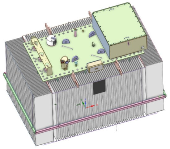
Figure 1.
The three-phase distribution transformer with corrugated tank walls.
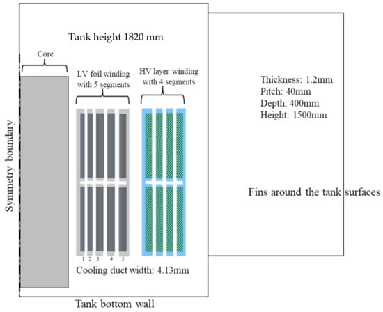
Figure 2.
Layout of winding in the tank cross-section.
3. Computational Fluid Dynamics
The computational fluid dynamics CFD was based on the commercial software package ANSYS-Fluent 2023 R2 [19], in which both heat transfer and fluid flow principles were transformed into a set of governing equations and solved with the methods of discretization and numerical iterations.
3.1. Geometry
The transformer geometry must be simplified for the CFD simulation. This was achieved by removing many components that can prolong the computational time without too much compensation of the accuracy. This simplification includes leads, cleats, structural components, axial and radial key spacers and sticks.
Furthermore, due to the significant differences in the thickness and length of fins, a large number of fine grids are required to calculate the flow over the walls and its heat transfer. Therefore, using an entire three-dimensional transformer model for CFD analysis would be computationally heavy and unrealistic. It is necessary to simplify appropriately so that conventional workstations can complete simulation calculations. The CFD simulation of the distribution transformer shown in Figure 1 was performed on a simplified model of a section containing 1/32 of one phase (which represents 1/96 of the total winding), and hence the same ratio of 1/96 losses was considered to represent the heat source. The tank, which has 198 fins in total, was modelled by taking 2 fins in the model. This number of fins represents 1/99 of the tank cooling capacity ratio that is equivalent to the loss ratio, as shown in Figure 3. The computation time required for one single case in the simplified 3D model could reach 14 h on an Intel Xeon Sliver 4110, 2.1 GHz, duo-processor-node with the total number of 36 physical cores running with Microsoft Windows.
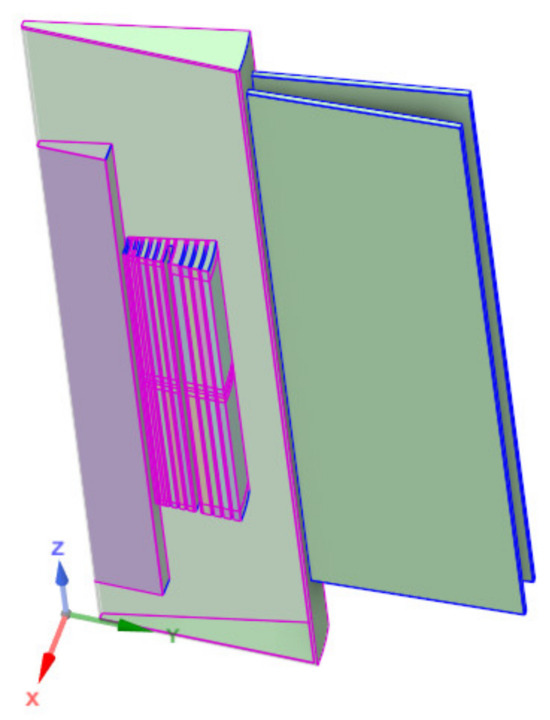
Figure 3.
Simplified axisymmetric 3D model of the transformer.
In this study, the windings were divided into several segments using cooling ducts as separators. These segments consist of conductors and insulating materials arranged systematically, enabling the use of equivalent thermal conductivity coefficients in all directions. The values of these equivalent coefficients can be obtained through formulas or finite-element calculations, allowing for reasonable reduction in the complexity of modelling winding details while still maintaining accuracy.
For foil windings, where conductors and insulating materials are arranged in an interleaved manner, the equivalent thermal conductivity coefficients in all three directions can be determined using the following formulas.
For the radial direction, it can be treated as a series connection. The thermal resistance R = R1 + R2, from which the equivalent thermal conductivity will be
For axial and circumferential directions, it can be treated as a parallel connection. The thermal resistance 1/R = 1/R1 + 1/R2, from which the equivalent thermal conductivity will be
where are the thickness of metal and insulation layer, respectively, and are the thermal conductivity of metal and insulation layer, respectively. is the equivalent thermal conductivity along the corresponding direction.
Due to the complexity of the supporting and insulating structures in the oil tank, the model cannot fully cover all details. Instead, the focus is mainly on the obstruction in the cooling duct, as it has the most significant impact on temperatures. The surfaces for cooling are partly blocked due to cooling duct collapsing and braces, which was considered by adding insulation sticks in the cooling ducts based on their actual volume proportion.
It is essential to ensure that the spacing, thickness and height of the heat-dissipating fins relative to the windings remain consistent with the actual model during the simplification process.
To better simulate the heat dissipation of fins, the model also includes an air domain based on the spatial size of the laboratory, which causes the region being solved to include fluids, solids and gases.
3.2. Meshing Setup
In fluid simulation, an appropriate mesh is crucial for obtaining accurate results. Particularly, inside the oil channels, a sufficiently refined mesh is required to capture boundary layer effects. The increase in the number of grids will significantly affect the speed of simulation calculations, while a small number of grids can lead to convergence problems and even result in distorted results. In this case, the size of the boundary layer mesh affects the definition of the global minimum size. Narrow oil channels have fluid solid interfaces on both sides, requiring the generation of boundary layers. Before generating the grid, we estimate that the Y-Plus value is less than 1, then the height of the grid nodes in the first layer should be less than 0.15 mm. In the oil passage with a width of 4.13 mm, 20 layers of prism are arranged, and it is obvious that the height of the first layer of grid is less than 0.1 mm.
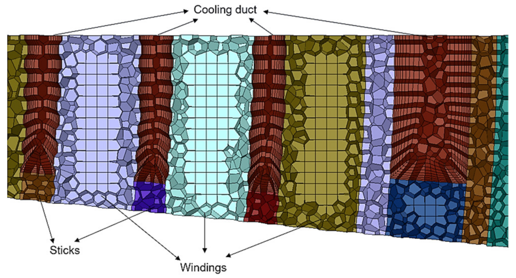
Ansys Fluent Meshing is used to generate the high-quality mosaic mesh with hexahedral dominant mesh topology, and prism layers are applied on all fluid–solid interfaces. The total number of volume mesh cells is around 24 million. The details of the cell mesh can be found in Figure 4.

Figure 4.
Mesh details.
3.3. Boundary Conditions
The boundary conditions were set as shown in Figure 5. The heat generation depends on the transformer losses, which are obtained through electromagnetic simulation software. These losses were assumed to be evenly distributed among all the winding sections and were further compounded by the effects of no-load loss and stray loss on the oil to fully consider the impact of total losses.
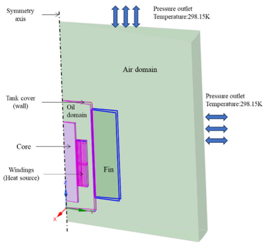
Figure 5.
Boundary conditions for CFD simulation.
The resistance of the winding is related to the temperature, which is defined in IEC 60076-1 Annex E [20]. When the current value remains constant, the loss value is proportional to the resistance. Therefore, in thermal simulation, it is reasonable to use a user-defined function to create the relation between loss and temperature, then the final convergence will be reached after number of iterations.
Following is an example to define the energy source for the HV section, the following code should be included in the udf file:
| #define p_hv_dc 93512.55 #define p_hv_eddy 839.73 #define type_con_hv 225 #define type_con_lv 225 DEFINE_SOURCE(energy_source_hv,c,t,dS,eqn) { real T,source; T = C_T(c,t); source = p_hv_dc*(type_con_hv+(T- 273.15))/(type_con_hv+refT)+p_hv_eddy*(type_con_hv+refT)/(type_con_hv+(T-273.15)); return source; } |
For the pressure outlet boundary for the air domain, the backflow temperature was set to room temperature: 298.15 K. We activated the DO model for radiation to consider the heat radiation to dissipate from the fins to the ambient air.
3.4. Solver
The simulation is conducted in a steady-state regime, focusing on the flow and temperature fields. The heat source is from the windings, with heat transferred through the oil to the oil tank walls. Heat is dissipated to the external air through convective heat transfer. Inside the oil tank, buoyancy-driven natural convection occurs due to temperature differences, causing the oil to flow from the bottom through the oil channels to the top, where its temperature gradually increases. It then flows back to the bottom through the fins’ side, and its temperature gradually decreases. The turbulence model chosen is the widely used shear stress transport SST k-ω turbulence model, which combines the best of k-ω which is suitable for the inner flow in the cooling ducts and the boundary layer of the inner and outer flows attached to the walls. It is suitable for low Re turbulence flow which is the case inside a natural cooled transformer. The SST can switch to a k-ε behavior in the free-stream regions where the adverse pressure gradients and separating flow may occur (exit from the top of transformer’s winding) and thereby avoids the common k-ω problem which is too sensitive to the inlet free-stream turbulence properties. In addition, the radiation model selected is the DO model. During the calculation process, in addition to the residual curve monitored by the software by default, key variables such as the average temperature of the winding and the oil are also continuously monitored. When all values of the residual curve are below 1 × 10⁻⁶ and the curve of the key variable remains stable, it is considered that the calculation has converged.
The properties of oil have significant influence on the thermal performance [21]. The transformer in this study uses mineral oil, and material properties are set based on the supplier’s provided data. Specific heat and thermal conductivity show negligible variation with temperature and can be treated as constants within the temperature range inside the tank. However, viscosity varies significantly with temperature, so a fitted formula is used as input. The density model adopts the Boussinesq approximation, which considers the fluid density temperature dependency through thermal expansion. The main properties of the mineral oil are provided in Table 1.

Table 1.
Mineral oil properties used in the CFD simulations.
The CFD solution was performed with refining the mesh while monitoring the convergence of a reference value, which is in this study the hot spot temperature of the top part of the LV winding. The CFD simulations provided a detailed and comprehensive analysis by revealing the temperature distribution of the oil and coil inside the transformer, as illustrated in Figure 6.
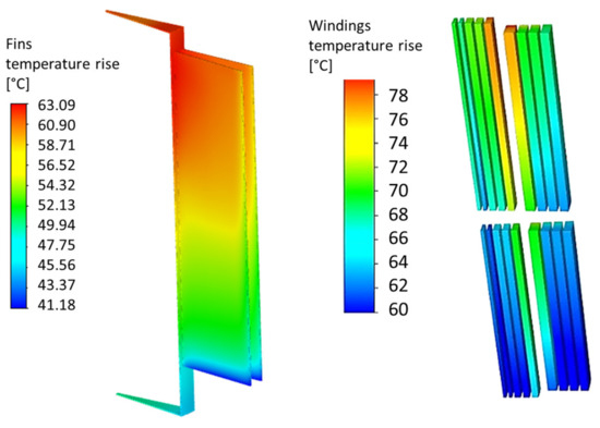
Figure 6.
Temperature distributions of the corrugated wall fins and winding.
4. Thermal–Hydraulic Model
The THM applies the heat and mass conservation principles together with the fluid pressure balance in closed flow loops. Each loop represents a winding (or a single layer of a winding) and the tank wall fins. The heat gained from the winding to the coolant oil is governed by the convection heat transfer coefficient and the heat dissipation is balanced with the total of the ohmic and eddy current losses [22,23]:
where
- —oil mass flow rate through winding [kg/s];
- —specific heat capacity of winding [J/ (kg K)];
- —top oil temperature rise in winding j[K];
- —bottom oil temperature rise [K].
The heat transferred into the oil will be dissipated through the tank wall fins into the ambient air which can then be calculated by integrating the differential energy equilibrium equation of oil filled in the fins [14,22]:
where
- —mean heat transfer coefficient of air [W/m2K];
- —fins surface area [m2];
- —mean oil temperature rise [K];
- —oil mass flow rate through fins [kg/s];
- —specific heat capacity of the oil in fins [J/(kg K)].
For the steady-state condition and applying the energy balance of the heat that enters the fins which shall be dissipated by the fins to the ambient [23,24], we obtain the following:
The THM solves the thermal hydraulic network in an iterative way. The stopping criteria are required to converge the calculation and reach the steady-state condition. These stopping criteria are the pressure equilibrium across all windings in analogy to the electrical parallel resistance and the assumption of the same oil speed across all fins. All these assumptions were validated using CFD simulations and then implemented in the THM to simplify the calculation.
To facilitate the modelling and swift the calculation time, the following assumptions were applied in the model:
- -
- Linear pressure and temperature distributions along the fins;
- -
- Equal flow rates through all fins. This is achieved by taking a loop over all fins and equally dividing the flow for each fin.
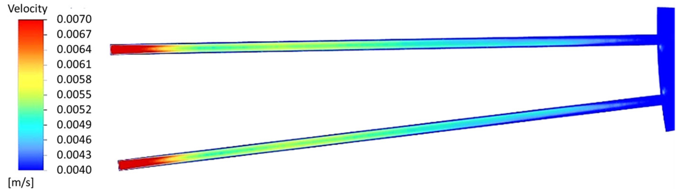
These assumptions were verified by performing CFD simulations. The CFD result shows that the linear pressure and temperature distributions along the fins are valid and hence can be used in the model. The validity of the assumption of equal temperature and flow rate across all fins was proven with the CFD by considering a middle height horizontal cross-section of the fins, as seen in Figure 7.

Figure 7.
Oil velocity distribution inside fins’ cross-section.
The heat from the winding to the oil is dissipated to the ambient air through two paths: tank walls (mainly through the cover) and tank wall fins. The tank cover area dissipated heat to the ambient at the reference top oil temperature rise TOT.
The oil circulation is driven by the thermal buoyancy force through the loops (windings and fins), and it is calculated by closed-loop integration of the density variation along the hydraulic height difference of the fins to the winding centers.
where
- —height difference between the vertical center of the fins and winding [m];
The pressure gain () can be simplified for the oil flow loops through each winding and fins to
where
- —oil volume expansion coefficient [1/K].
The pressure drop is evaluated by considering the major and minor pressure drops along the oil flow through all windings and fins.
where
- —length of oil paths [m];
- —hydraulic diameter [m];
- );
- —frictional factor (laminar flow in ducts);
- —oil density [kg/m3];
- —oil velocity [m/s].
The Reynolds number is needed for calculating pressure drops, as
where
- —dynamic viscosity of oil [kg/(m s)].
The minor losses along the oil flow through the winding and fin bends, branches and any other direction-changing parts are calculated as
where
- —loss coefficient specifically for each type of flow direction changing.
We sum the pressure drops obtained as
Then, the pressure gain should be equal or greater than the pressure-drop:
In analogy to electrical circuit, the stopping criteria are valid for the application of Kirchhoff’s law for each winding as a resistor branch connected to the fins as the main sink branch.
In addition, the assumption of equal pressure drop across the windings must be fulfilled for the convergence of the model with analogy to the equal voltage drop of parallel branches of an electrical circuit.
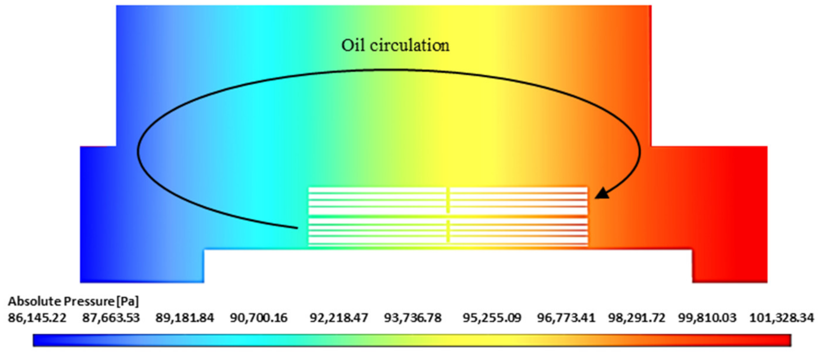
The assumption of equal pressure drops across parallel windings (LV and HV) is verified with CFD simulation. Figure 8 shows the calculated pressure drop along the two main windings that are thermally and hydraulically coupled to the corrugated wall fins. Results show that the pressure difference along both the LV and HV windings is the same.
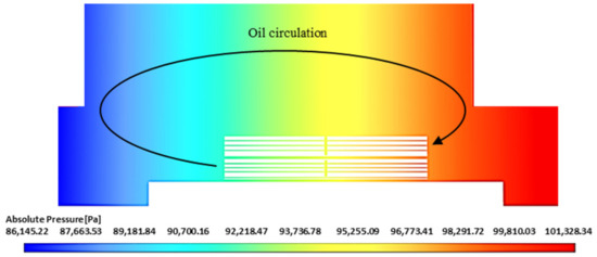
Figure 8.
Pressure drop along the windings and tank oil including one fin (right side is the bottom of the transformer).
Different insulating liquids were considered in the model by changing the liquid properties (density, viscosity, specific heat), and all properties were considered to be variable with temperature. However, in the current study, the measurement validation was only applied on a mineral oil filled distribution transformer.
Until this calculation stage, the model is balanced, and the iteration must converge to a solution of temperatures and mass flow rates without considering the cooling capacity of the corrugated tank wall to dissipate the generated heat inside the transformer to the ambient. For that, the energy generated must be balanced with the energy dissipated by the corrugated wall. This energy balance requires an external iteration loop for the average oil temperature until reaching the balance state between the energy which enters the radiator after subtracting the energy dissipated through the tank cover.
The axially stacked winding was handled by distributing the losses across the axial winding’s blocks to calculate the actual mass flow rate, while considering the whole cooling duct across the active and passive windings to calculate the actual pressure drop. The no-load and load loss components and the other stray losses outside winding were added to the main windings losses to reflect the heat-run test.
Solving the set of equations for each winding (or radial section),
The thermal model shall solve the set of linear equations by iteration for temperatures and their corresponding flow rates per winding and set of wall fins (radiator) until fulfilling the stopping criteria. Figure 9 demonstrates the thermal–hydraulic network procedures.
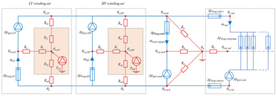
Figure 9.
Thermal–hydraulic network of main windings, tank and radiator.
5. Heat-Run Test
The thermal analysis was applied on an actual manufactured transformer that underwent heat-run in the routine factory acceptance test (FAT). Temperature rise measurement for the unit was carried out in accordance with the IEC standards. The transformer was equipped with several temperature sensors to monitor the temperature of the oil, whereas the temperature rises in the low-voltage and high-voltage windings were calculated through the cooling down resistance method.
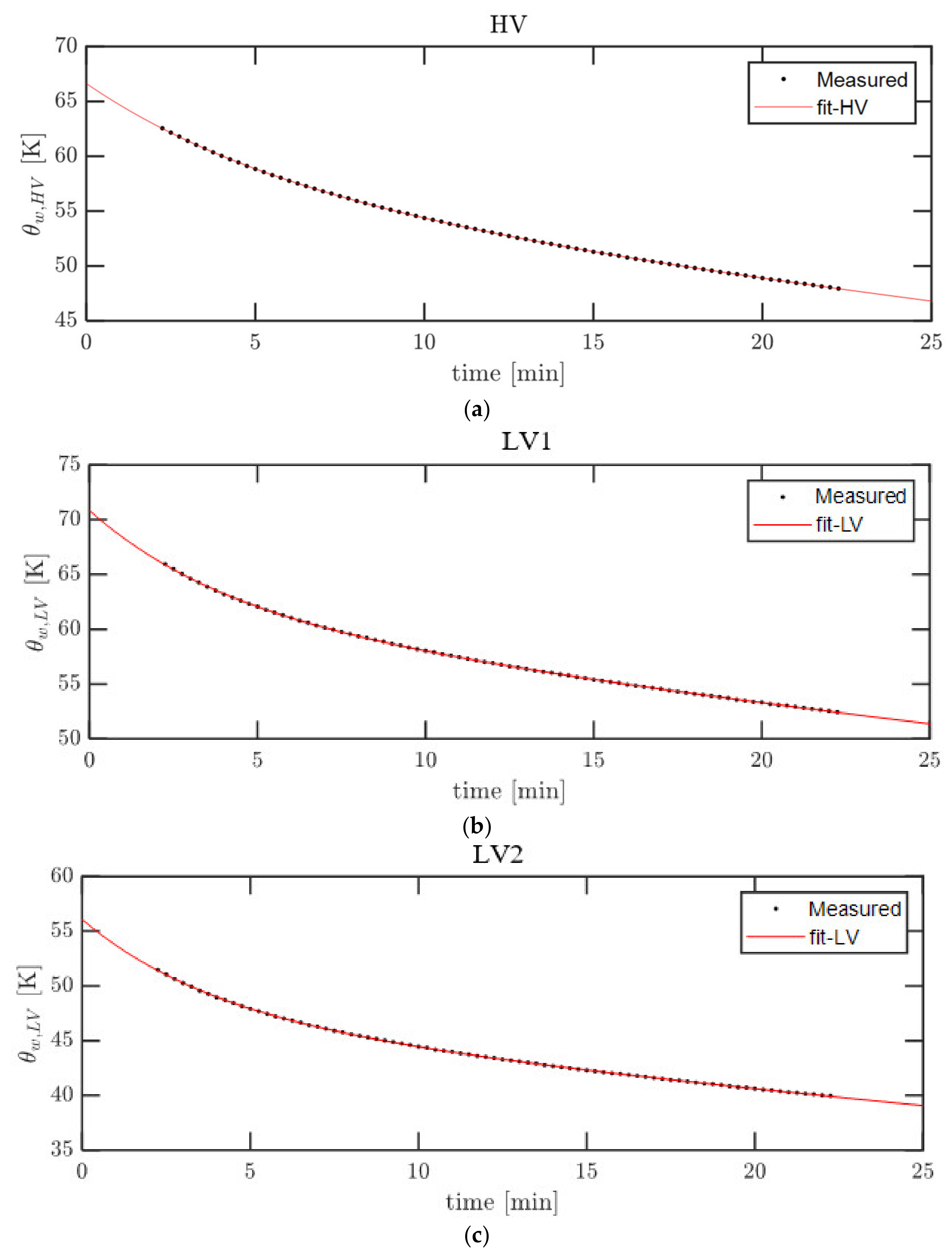
The heat-run was performed according to IEC 60776-2 [25]. Firstly, the top oil of the unit was measured with the injection of total loss current until reaching stability. This step can be terminated when the top oil temperature changing rate falls below 1 K per hour and remains there for a period of three consecutive hours. Then, the test should be continued without a break with the current reduced to the rated current until reaching a reduced and stabilized top oil temperature. The winding average temperatures are then derived from the measured electric resistance variation. The temperature rises in the upper part of the LV (LV1) and the lower part (LV2) were calculated separately, while the temperature rise in the HV represents the average value of the whole HV winding. The temperature rises in the windings are calculated using exponential function fitting for the cooling curves, see Figure 10.
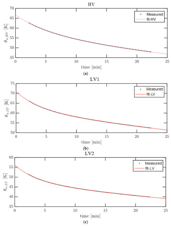
Figure 10.
Cooling curves analysis to calculate the average winding temperature rise in (a) HV winding, (b) LV1 winding and (c) LV2 winding.
The results of the heat-run test were compared with both the CFD and THM calculation approaches as presented in Table 2. In general, the results are well matched between tests for CFD and THM. But for the test value of LV2-AVG (the bottom section of the LV), the CFD and THM show an 8–11 K higher temperature rise than the measured value, which requires further diagnostic attention.
Table 2.
Test and calculation results.
6. Conclusions
The current study presents a comprehensive analysis of the cooling efficiency of an oil-filled distribution transformer using developed approaches of CFD and THM calculations. The results of both calculation methods were compared with the heat-run test on a case study of an oil-filled distribution transformer. A satisfactory matching of the key thermal performance parameters was found which proves the reliability of both approaches in calculation of the thermal performance. Nevertheless, the THM proves to have both accuracy and swift calculation compared to CFD that makes it more recommended for daily designs.
On the other hand, the CFD is still a very useful tool for calculation of the thermal performance for validation studies, deep insight into the thermal behavior and to calculate special designs with complicated geometry. However, the THM inhibits physical assumptions that need to be validated with CFD. Furthermore, the THM requires the implementation of parameters and corrections factors to be generated with CFD to facilitate the calculation.
This study is expected to be a valuable reference for improving the thermal performance and operation efficiency of distribution transformers and, eventually, aims to provide engineers with an effective tool to design the most efficient and reliable corrugated tank wall distribution transformers.
Author Contributions
Conceptualization, C.W. and Q.S.; methodology, C.W. and A.A.-A.; software, C.W. and A.A.-A.; validation, C.W. and A.A.-A.; formal analysis, C.W. and A.A.-A.; investigation, C.W., Q.S. and A.A.-A.; resources, W.W.; writing—original draft preparation, C.W. and A.A.-A.; writing—review and editing, W.W. and A.A.-A.; visualization, A.A.-A.; supervision, Q.S. and A.A.-A.; project administration, Q.S. and A.A.-A. All authors have read and agreed to the published version of the manuscript.
Funding
This research received no external funding.
Data Availability Statement
The original contributions presented in the study are included in the article, further inquiries can be directed to the corresponding author.
Conflicts of Interest
Authors Chunping Wang, Qingjun Sun, Ali Al-Abadi and Wei Wu were employed by the company Hitachi Energy.
References
- Radakovic, Z.; Sorgic, M.; Van der Veken, W.; Claessens, G. Ratings of oil power transformer in different cooling modes. IEEE Trans. Power Deliv. 2012, 27, 618–625. [Google Scholar] [CrossRef]
- Torriano, F.; Chaaban, M.; Picher, P. Numerical study of parameters affecting the temperature distribution in a disc-type transformer winding. Appl. Therm. Eng. 2010, 30, 2034–2044. [Google Scholar] [CrossRef]
- Wu, W.; Wang, Z.; Revell, A.; Iacovides, H.; Jarman, P. Computational fluid dynamics calibration for network modeling of transformer cooling oil flows-part I heat transfer in oil ducts. IET Electr. Power Appl. 2011, 6, 19–27. [Google Scholar] [CrossRef]
- Gastelurrutia, J.; Ramos, J.C.; Larraona, G.S.; Rivas, A.; Izagirre, J.; Del Río, L. Numerical modelling of natural convection of oil inside distribution transformers. Appl. Therm. Eng. 2011, 31, 493–505. [Google Scholar] [CrossRef]
- Archambeau, F.; Mechitoua, N.; Sakiz, M. A finite volume method for the computation of turbulent incompressible flows-industrial applications. Int. J. Finite Vol. 2004, 1, 1–62. [Google Scholar]
- EKranenborg, E.J.; Olsson, C.O.; Samuelsson, B.R.; Lundin, L.Å.; Missing, R.M. Numerical study on mixed convection and thermal streaking in power transformer windings. In Proceedings of the 5th European Thermal-Science Conference, Eindhoven, The Netherlands, 18–22 May 2008. [Google Scholar]
- Taghikhani, M.; Gholami, A. Prediction of hottest spot temperature in power transformer windings with non-directed and directed oil-forced cooling. Electr. Power Energy Syst. 2009, 31, 356–364. [Google Scholar] [CrossRef]
- Skillen, A.; Revell, A.; Iacovides, H.; Wu, W. Numerical prediction of local hot-spot phenomena in transformer windings. Appl. Therm. Eng. 2012, 36, 96–105. [Google Scholar] [CrossRef]
- Weinläder, A.; Wu, W.; Tenbohlen, S.; Wang, Z. Prediction of the oil flow distribution in oil-immersed transformer windings by network modelling and CFD. IET Electr. Power Appl. 2011; provisionally accepted. [Google Scholar]
- Oliver, A.J. Estimation of transformer winding temperatures and coolant flows using a general network method. Proc. Inst. Elect. Eng. Pt. C 1980, 127, 395–405. [Google Scholar] [CrossRef]
- Yamaguchi, M.; Kumasaka, T.; Inui, Y.; Ono, S. The flow rate in a self-cooled transformer. IEEE Trans. Power App. Syst. 1981; PAS-100, 956–963. [Google Scholar]
- Declercq, J.; Van Der Veken, W. Accurate hot spot modeling in a power transformer leading to improved design and performance. In Proceedings of the IEEE Transmission and Distribution Conference, New Orleans, LA, USA, 11–16 April 1999. [Google Scholar]
- Campelo, H.; Lopez-Fernandez, X.M.; Picher, P.; Torriano, F. Advanced Thermal Modelling Techniques in Power Transformers. Review and Case Studies. In In Proceedings of the Advanced Research Workshop on Transformers, Baiona, Spain, 28–30 October 2013. [Google Scholar] [CrossRef]
- Radakovic, Z.R.; Sorgic, M.S. Basics of Detailed Thermal-Hydraulic Model for Thermal Design of Oil Power Transformers. IEEE Trans. Power Deliv. 2010, 25, 790–802. [Google Scholar] [CrossRef]
- Zhang, J.; Li, X. Oil cooling for disk-type transformer windings-Part I: Theory and model development. IEEE Trans. Power Del. 2006, 21, 1318–1325. [Google Scholar] [CrossRef]
- Gamil, A.; Al-Abadi, A.; Schatzl, F.; Schlücker, E. Theoretical and Empirical-Based Thermal Modelling of Power Transformers. In Proceedings of the IEEE International Conference on High Voltage Engineering and Application (ICHVE), Athens, Greece, 10–13 September 2018; pp. 1–4. [Google Scholar]
- Amoiralis, E.I.; Tsili, M.A.; Kladas, A.G.; Souflaris, A.T. Distribution transformer cooling system improvement by innovative tank panel geometries. IEEE Trans. Dielectr. Electr. Insul. 2012, 19, 1021–1028. [Google Scholar] [CrossRef]
- Campos, A.R.T.; Mariscal, I.C.; Hernandez, S.G. Simulation of a distribution transformer. WSEAS Trans. Fluid Mech. 2012, 7, 106–115. [Google Scholar]
- ANSYS. Fluent User’s Manual, Fluent 22.2; ANSYS, Inc.: Canonsburg PA, USA, 2022. [Google Scholar]
- IEC 60076-1:2011; Power Transformers—Part 1: General. IEC: Geneva, Switzerland, 2011.
- Santisteban, A.; Piquero, A.; Ortiz, F.; Delgado, F.; Ortiz, A. Thermal Modelling of a Power Transformer Disc Type Winding Immersed in Mineral and Ester-Based Oils Using Network Models and CFD. IEEE Access 2019, 7, 174651–174661. [Google Scholar] [CrossRef]
- Gamil, A.; Al-Abadi, A.; Schiessl, M.; Schatzl, F.; Schlucker, E. Improvements on Thermal Performance of Power Transformers: Modelling and Testing. In Proceedings of the 6th International Advanced Research Workshop on Transformers (ARWtr), Cordoba, Spain, 7–9 October 2019; pp. 13–18. [Google Scholar] [CrossRef]
- Al-Abadi, A.; Wu, W.; Yadava, J. Thermal Performance Analysis of Liquid-Filled Large Distribution Transformers by Enhancing Thermal Hydraulic Modelling with CFD. In Proceedings of the Cigre SC A2 & 6th International Colloquium. Transformer Research and Asset Management, Split, Croatia, 29 November–2 December 2023. [Google Scholar]
- Wang, C.; Sun, Q.; Al-Abadi, A.; Wu, W. Computational Fluid Dynamics and Thermal Hydraulic Modelling Approaches for Calculation of Thermal Performance of Oil-Filled Distribution Transformers with Corrugated Walls. In Proceedings of the Cigre SC A2 & 6th International Colloquium. Transformer Research and Asset Management, Split, Croatia, 29 November–2 December 2023. [Google Scholar]
- IEC 60076-2:2011; Power Transformers—Part 2: Temperature rise for Liquid-Immersed Transformers. IEC: Geneva, Switzerland, 2011.


Disclaimer/Publisher’s Note: The statements, opinions and data contained in all publications are solely those of the individual author(s) and contributor(s) and not of MDPI and/or the editor(s). MDPI and/or the editor(s) disclaim responsibility for any injury to people or property resulting from any ideas, methods, instructions or products referred to in the content. |
© 2024 by the authors. Licensee MDPI, Basel, Switzerland. This article is an open access article distributed under the terms and conditions of the Creative Commons Attribution (CC BY) license (https://creativecommons.org/licenses/by/4.0/).