Abstract
In response to increasingly stringent global environmental policies, this study addresses the pressing need for accurate prediction models of CO2 emissions from vehicles powered by alternative fuels, such as compressed natural gas (CNG). Through experimentation and modelling, one of the pioneering CO2 emission models specifically designed for CNG-powered vehicles is presented. Using data from chassis dynamometer tests and road assessments conducted with a portable emission measurement system (PEMS), the study employs the XGBoost technique within the Optuna Python programming language framework. The validation of the models produced impressive results, with R2 values of 0.9 and 0.7 and RMSE values of 0.49 and 0.71 for chassis dynamometer and road test data, respectively. The robustness and precision of these models offer invaluable information to transportation decision-makers engaged in environmental analyses and policymaking for urban areas, facilitating informed strategies to mitigate vehicular emissions and foster sustainable transportation practices.
Keywords:
vehicles; CNG; CO2; emission; PEMS; chassis dynamometer; pollution; artificial intelligence 1. Introduction
Global policy aims to minimise the increasing greenhouse effect. The average temperature on Earth in the past year, 2023, was the highest recorded [1,2]. A case in point is the European Union’s policy striving to reduce CO2 emissions by 90% by 2040 compared to 1990, with 2050 set as the beginning of complete climate neutrality [3,4]. Such circumstances require the search for solutions across various levels and industries. The CO2 emissions from transportation are particularly noteworthy, accounting for approximately 25% of the total global anthropogenic emissions of this component [5,6]. Road transport is responsible for more than 70% of total CO2 emissions from the transportation sector [7,8]. Consequently, newer vehicle designs are gradually introduced to reduce CO2 emissions, with imminent compliance with EURO 7 standards [9,10]. The increasingly popular use of electric propulsion systems is seen as a means of reducing vehicle emissions. However, the rapid growth of this type of propulsion is not uniform across regions due to various constraints, including infrastructure and economic limitations [11,12]. Therefore, alternative fuels and solutions for applications in transportation are necessary [13,14].
One such fuel is CNG, which can serve as a renewable fuel, a highly desirable characteristic. Burning this fuel in vehicle engines reduces CO2 emissions by 20% [15,16]. CNG, or compressed natural gas, represents an alternative fuel used in road transportation, characterised by a range of environmental and economic benefits [17]. It consists primarily of methane, making it a fuel with lower carbon content compared to traditional fossil fuels such as gasoline or diesel [18]. Consequently, burning CNG generates significantly lower emissions of carbon dioxide (CO2) and other harmful substances, such as nitrogen oxides (NOx) and particulate matter [19,20]. CNG fuel is primarily used in vehicles travelling on the road, including passenger cars, buses, and commercial fleets, such as taxis or utility vehicles [21]. The popularity of CNG is particularly growing in countries where intensive efforts are being made to reduce air pollution emissions and reduce dependence on fossil fuels. European countries such as Italy, Germany, the Netherlands, and Sweden are leaders in the adoption and promotion of CNG-powered vehicles [22,23]. Many scenarios are also being created for the replacement, for example, of public vehicle fleets, which are currently powered by diesel engines, with engines powered by CNG [24]. In Poland, there is also a noticeable increase in interest in this type of fuel, especially in the public transportation sector and commercial vehicle fleets [25,26]. However, efforts are still being made to identify why the development of alternative propulsion systems in Poland is not progressing as dynamically as in other countries [27]. An increasing number of countries around the world, both developed and developing, are considering the introduction of CNG fuel as part of their strategies to reduce emissions from road transportation. However, to fully realise the environmental benefits of CNG vehicles, it is essential to develop robust models capable of accurately predicting their CO2 emissions under real-world driving conditions.
The essence of employing emission models, especially for CO2, in road analyses lies in their ability to forecast and assess the impact of vehicles on the environment accurately and comprehensively. The development of such models can be based on various methods, including chassis dynamometer tests and emissions monitoring during real-world driving conditions using a portable emission measurement system (PEMS) [28]. During chassis dynamometer tests, the vehicle is placed on a special platform, allowing the simulation of various driving conditions. Emissions, including CO2, are recorded during the test, allowing the development of predictive models based on the relationship between engine operating parameters and CO2 emissions. However, the PEMS system enables the monitoring of vehicle emissions under real driving conditions on the road. In recent years, there has been a significant increase in the popularity of mobile devices for measuring exhaust emissions, and they currently dominate in research studies [29,30]. Data on speed, acceleration, load, and emissions are collected during normal vehicle operation. Based on these data, emission models can be developed, taking into account various factors influencing CO2 emissions depending on road conditions and driver behaviour. It is worth noting that despite the existence of emission models for vehicles powered by conventional fuels such as gasoline or diesel, the process of creating emission models for CNG-powered vehicles is relatively underdeveloped and poorly described in the scientific literature. Therefore, more research and analysis are needed to develop effective methods for modelling CO2 emissions from CNG-powered vehicles, which would allow a more comprehensive understanding of the impact of these vehicles on the environment and support decision-making regarding transportation and environmental policy.
There are a very limited number of studies that address the issue of emissions from CNG-powered vehicles, and even fewer studies that focus on modelling emissions from this type of fuel. The only study that addresses the modelling of emissions from a CNG-powered vehicle is [31]. In this study, the research focuses on the utilisation of a hybrid fuel for diesel engine operation. The diesel engine is modified to run on a hybrid of diesel and compressed natural gas (CNG). Using a four-stroke, single-cylinder diesel engine operating under varying load and speed conditions, emission characteristics are measured to develop a Manhattan K-nearest neighbour (MKNN) technique. The MKNN model is designed to effectively analyse and predict torque, brake power, exhaust emissions, and brake-specific fuel consumption (BSFC). This study presents a brief investigation that shows the predictive capabilities of a simple model for CO, CO2, NOx, and O2. The modelling refers to a diesel engine that can also be powered by CNG. The number of existing studies on the topic of CNG-powered vehicle propulsion and their emissions, according to the Web of Science Core Collection, is minimal, with only 920 results retrieved for the search terms “CNG” and “vehicle”. As mentioned earlier in this paragraph, no work has been found for the search terms “CNG”, “vehicle”, and “model”. However, concerning the analysis of the available literature, it is worth noting that the number of studies focussing on emissions modelling, especially using artificial intelligence methods, is increasing. There are several studies that address emissions modelling for vehicles powered by gasoline [32,33], diesel [34,35], LPG [36,37] and hybrid combinations thereof [38].
Following the literature review, this paper addresses key issues related to modelling CO2 emissions for vehicles powered by CNG. In this context, it is worth emphasising that despite the existence of many emission models for conventional fuels such as gasoline or diesel, emission models for CNG-powered vehicles are still in an embryonic state. Shaping urban transport policy in the context of future fuels and the emissions/energy consumption generated by vehicles, therefore, requires the development of accurate emission prediction models for CNG-powered vehicles as well, considering that their percentage share in some countries is significant and still growing. Due to the existing research gap in the literature on modelling emissions of CNG-powered vehicles, this study addresses this topic. Input data for creating the CO2 emissions model were collected using two approaches. The first approach involved chassis dynamometer tests and the generation of vehicle motion and CO2 emission data. The second approach involved conducting road tests using the PEMS under real-world traffic conditions. This situation allowed for a comparison of the two approaches to emission modelling in the study, providing cognitive value to the field. Furthermore, the study presents potential applications of the models developed for a dedicated application capable of generating CO2 emission maps for vehicles powered by CNG, which constitutes a novelty in the analysed topic area. The tools and models developed can be utilised for environmental and infrastructural analyses regarding the applicability of this alternative fuel as a substitute for conventional fuels in road transportation.
Using advanced statistical techniques and machine learning algorithms, the objective is to uncover the intricate relationships between key driving parameters, vehicle characteristics, and CO2 emissions. The insights derived from the modelling efforts will not only improve the understanding of the factors influencing CO2 emissions from CNG vehicles but will also guide the formulation of strategies to diminish their environmental impact. The work was carried out in the Python programming environment using the Optuna framework, which facilitated the optimisation of the model hyperparameters. The XGBoost technique was chosen for model training, providing the ability to produce precise and reliable predictive models for the examined scenario.
Through a synthesis of empirical analysis and predictive modelling, valuable insights are aimed at supporting policymakers, industry stakeholders, and researchers in their efforts to advocate for the adoption of cleaner and more sustainable transportation technologies. Ultimately, the objective is to contribute to the progression of knowledge in this pivotal field and to support the transition toward a greener and more environmentally friendly transportation system.
2. Methods
The research methodology is based on several steps. The aim of the study is to develop CO2 emission models for CNG-powered vehicles as one of the first available in the literature on a microscale. The models were created based on road tests and laboratory tests conducted on a chassis dynamometer located at the Rzeszow University of Technology. Data analysis and model development were carried out using the Python programming language, particularly within the Optuna framework. The overall workflow is depicted in Figure 1.
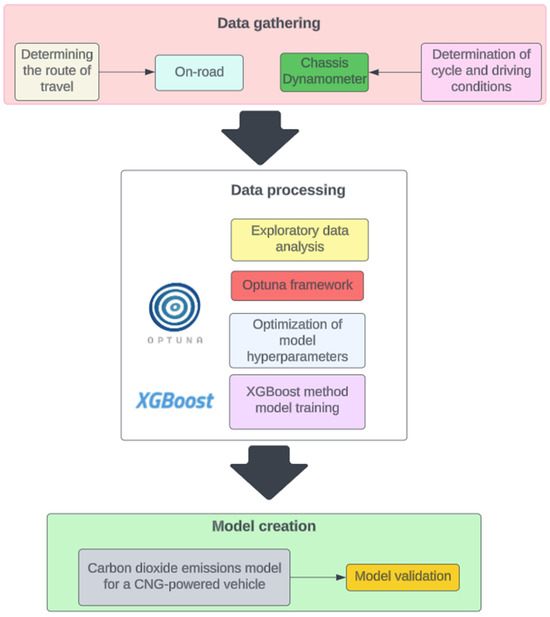
Figure 1.
Simplified workflow.
The first step involved conducting research on the vehicle using emission measurement techniques, particularly for CO2. Measurement technology itself varies between road tests and chassis dynamometer tests due to different measurement techniques for the devices used.
For the engine dynamometer part, the research was carried out under controlled climatic conditions according to the New European Driving Cycle (NEDC), which was the applicable road test for the vehicle under study. The tests were carried out on the Zoellner ROADSIM 48 chassis dynamometer, manufactured by AVL (Graz, Austria), housed in a climatic chamber. The AVL climatic chamber enables the maintenance of the temperature in the range of −20 to +30 °C. The AVL CVS i60 dilution system and the AVL AMA i60 exhaust analysis system were used at the measurement station. The measurement of CO2 emission from the exhaust was performed using a constant volume sampling system (CVS i60) system. The CVS i60 system operates by maintaining a consistent volume of gas samples during the measurement process. This ensures that the collected data accurately represent the concentration of CO2 emitted from the exhaust. Before the test began, the exhaust gas analysis system was calibrated.
Road tests were performed using the Horiba OBS-2200 Portable Emission Measurement System (PEMS) (Horiba, Kyoto, Japan) for the route depicted in Figure 2. The method of measuring CO2 from PEMS using the non-dispersive infrared (NDIR) technique involves the utilisation of infrared light to detect the presence and concentration of CO2 in the vehicle exhaust. In this technique, the PEMS system emits infrared light through the exhaust gas sample [39]. CO2 molecules in exhaust absorb specific wavelengths of infrared light, which are characteristic of CO2. By analysing the amount of infrared light absorbed by CO2 molecules, the NDIR technique can accurately quantify the concentration of CO2 in the exhaust gas stream. This method provides a reliable and real-time measurement of CO2 emissions during road driving conditions, allowing a comprehensive assessment of vehicle emissions and their environmental impact. The investigated route was approximately 35 km long and included various driving characteristics, that is, urban, suburban, and highway driving.
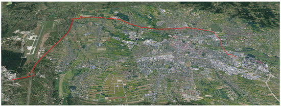
Figure 2.
View of the surveyed route used for CO2 measurement during road tests (red line).
The temperature for the NEDC test was 25 °C, similar to external conditions applied to road tests carried out with PEMS. The technical parameters of the investigated CNG-powered vehicle are presented in Table 1.

Table 1.
Selected Technical Parameters of the Investigated CNG-Powered Vehicle.
This comparison for creating CO2 emission models under two different testing conditions and measurement techniques will be a valuable source of knowledge for further research on these aspects of modelling, especially CO2 emissions from CNG-powered vehicles. Data from the dynamometer and the PEMS system were saved in .csv format at a frequency of 1 Hz. In the scope of CO2 emission modelling, the key was the selection of parameters that would serve as explanatory variables. For this purpose, the speed and acceleration of the vehicle were chosen. The selection of these parameters is justified by the goal of obtaining the most universal model. Speed data can be obtained during driving or during simulations in various software programs.
The saved data were preliminarily analysed and then used to create the CO2 emission model. For this purpose, as mentioned above, data for vehicle speed, acceleration and CO2 emissions themselves as dependent variables were necessary. Data analysis and modelling were performed using the Python programming language. Python is a versatile interpreted programming language with clear syntax, making it a popular choice in the scientific world. With its rich standard library and specialised packages such as NumPy and TensorFlow, Python enables researchers to analyse data, perform machine learning, and process signals. The Optuna framework was used to develop the models. The Optuna framework provides efficient methods for hyperparameter optimisation, enabling the fine-tuning of model parameters to enhance predictive accuracy. Integrating these tools with the XGBoost technique facilitates the creation of precise and reliable predictive models for CO2 emissions from CNG-powered vehicles. Justifying the selection of the XGBoost technique and discussing its advantages for this application is paramount to understanding the efficacy of the methodology in the modelling of CO2 emissions for CNG-powered vehicles. XGBoost, an implementation of gradient-boosting algorithms, stands out for its exceptional performance in handling structured data and addressing complex regression tasks, making it well-suited for modelling emissions from diverse vehicle types under real-world driving conditions. One of its key advantages lies in its ability to handle nonlinear relationships between input variables and output targets, allowing for more accurate predictions of CO2 emissions. Furthermore, XGBoost offers robustness against overfitting and is able to capture intricate patterns in the data, contributing to the development of reliable predictive models [40]. In addition, its scalability and efficiency make it suitable for processing large data sets efficiently, which is crucial for analysing emissions from a diverse range of vehicles in varying driving scenarios. This approach not only leverages state-of-the-art methodologies but also ensures reproducibility and scalability in the modelling process.
3. Results
The work was carried out in the Google Colab environment. Google Colab is a platform for working with Jupyter notebooks in the cloud, enabling scientists and programmers to utilise Google’s computational resources flexibly and conveniently. By allowing Python code execution in a web browser environment, Colab facilitates collaboration on projects, code sharing, and presentation of results. Additionally, the availability of pre-installed libraries such as TensorFlow, PyTorch, and scikit-learn simplifies data analysis and machine learning without the need to install additional software [41]. The open nature of the platform and its integration with Google services such as Google Drive and Google Cloud have made Google Colab a popular tool in research and educational environments [42].
3.1. Exploratory Data Analysis
Exploratory data analysis (EDA) involves creating visualisations of the relationships between parameters in the data set. To achieve this, a set of scatter plots and histograms was generated for all combinations of variables. Pairplot graphs also allow for an initial assessment of the data distribution, identification of outliers, and detection of potential patterns or nonlinear relationships. Such a preliminary analysis enables a better understanding of the data complexity and facilitates informed decisions for fitting future models. In Figure 3, a plot is presented depicting the dependencies among the investigated parameters for both the dynamometer and road tests.
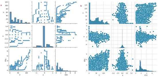
Figure 3.
The plot illustrating the relationships between the investigated parameters for modelling CO2 emissions from a CNG-powered vehicle is presented below for (a) dynamometer data and (b) on-road data.
The data used to model CO2 emissions from the dynamometer tests comprised 1229 records, while the on-road data consisted of 5591 records. On the basis of Figure 3, one can primarily observe the formation of patterns for the dynamometer data. This is attributed to the driving conditions of the road cycle simulated on the dynamometer, which assumes constant acceleration moments and driving at preset speeds, as reflected in scatter plots and histograms. Based on this, it can be assumed that the created model will accurately predict CO2 emissions for these driving conditions. However, there may be an issue with dynamic conditions due to the lack of a sufficient number of input data samples for model training.
For on-road data, a wide variety of collected data is evident, influenced by diverse traffic conditions during driving.
In the subsequent stage of exploratory data analysis (EDA), the influence of explanatory variables on the target value of CO2 was examined. After data verification and analysis, it was determined that the XGBoost method would exhibit the best predictive capabilities. The SHAP value plot (Figure 4) was utilised for this verification. Using the SHAP library (SHapley Additive exPlanations), the impact of individual features on the model predictions was understood. After training the XGBoost model on the training data, a SHAP explainer object was created to calculate SHAP values for the test data. Analysing these values enabled the identification of significant features and an understanding of their impact on the model results. Subsequently, SHAP plots were generated to visually represent the significance of each variable for the model predictions. In SHAP plots, different colours correspond to different feature values. The red colour indicates a high feature value contributing to higher model predictions, while the blue colour denotes a low feature value reducing the prediction. The more intense the colour (red or blue), the greater the impact of the feature on the model prediction. The x-axis represents the SHAP value for each feature, while the y-axis represents the features.
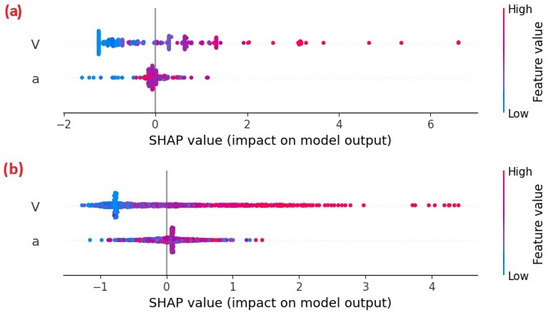
Figure 4.
SHAP value plot for (a) chassis dynamometer data and (b) on-road data.
3.2. Model Creation
To create CO2 emission models for CNG-powered vehicles, the Optuna framework was utilised. Optuna is an open-source tool for automatic hyperparameter tuning, enabling effective optimisation of machine learning models. It is a popular library in the machine learning world, offering advanced features such as various hyperparameter exploration strategies, integration with different modelling libraries like scikit-learn or TensorFlow, and flexible configuration of optimisation algorithms [43]. Optuna allows users to define custom objective metrics, constraints, and evaluation strategies, tailoring the optimisation process to specific applications. Using tree-based algorithms, sequential optimisation, and other methods, Optuna can effectively search the hyperparameter space and find optimal model configurations, speeding up the model creation process and enhancing its performance [44].
For hyperparameter optimisation purposes, the XGBoost regression model was selected. The optimisation process involved searching the hyperparameter space to minimise the root mean square error (RMSE) in the test set. To achieve this, optimisation algorithms such as random search and trial scheduling were employed to find the best sets of hyperparameters. The objective function included sets of model parameters, such as booster type, regularisation coefficients, maximum depth, learning rate, and others. The optimisation algorithm conducted experiments based on these parameters, evaluating their impact on the model’s performance and adjusting them in each iteration. Upon completion of the optimisation process, optimal hyperparameters were obtained, allowing the best performance of the XGBoost model in regression target prediction.
Figure 5 presents visualisations of hyperparameter optimisation results using the Parallel Coordinates Plot methodology. This tool helps to analyse optimisation results by allowing simultaneous comparison of multiple hyperparameters for each trial. Each line in the plot represents one study, and each axis corresponds to one of the hyperparameters. The colour and thickness of the lines can be used to visualise the objective function values for each test. Interpretation of this plot allows us to understand which combinations of hyperparameters were more effective in achieving the best results.
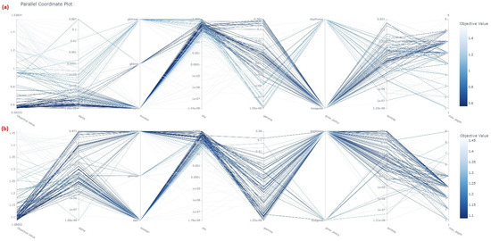
Figure 5.
Parallel Coordinates Plot: (a) chassis dynamometer data and (b) on-road data.
Figure 6 is used to visualise the importance of hyperparameters based on the optimisation results. Each bar on the chart represents the importance of a specific hyperparameter in the context of the achieved results. The higher the bar, the greater the influence of that hyperparameter on the final value of the objective function. Analysis of this chart allows for the identification of key hyperparameters that have the greatest impact on the model’s performance.
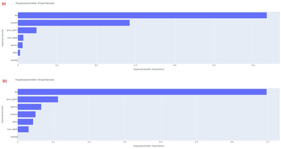
Figure 6.
Charts depicting the importance of hyperparameters: (a) chassis dynamometer data and (b) on-road data.
Based on Figure 5 and Figure 6, it can be observed that both for chassis dynamometer data and on-road data, the most significant hyperparameter is eta. This is the learning rate parameter that determines the speed at which the model learns during each iteration. High values of this parameter for both the chassis dynamometer and on-road data lead to fast learning models. Particularly for chassis dynamometer data, the booster parameter is also of high importance. It defines the type of model used in the XGBoost library. The second most important hyperparameter for on-road data is grow_policy, which determines the tree growth strategy during training. All these hyperparameters influence the quality, training time, and effectiveness of the model In dealing with overfitting issues.
Below, for Algorithm 1, a code snippet is presented that is used for hyperparameter optimisation with Optuna.
| Algorithm 1. Fragment of the CO2 emission modelling code for hyperparameter optimisation. |
| dtrain = xgb.DMatrix(X_train, label = y_train) dtest = xgb.DMatrix(X_test, label = y_test) def objective(trial): param = { ‘objective’: ‘reg:squarederror’, ‘eval_metric’: ‘rmse’, ‘verbosity’: 0, ‘booster’: trial.suggest_categorical(‘booster’, [‘gbtree’, ‘gblinear’, ‘dart’]), ‘lambda’: trial.suggest_loguniform(‘lambda’, 1 × 10⁻⁸, 1.0), ‘alpha’: trial.suggest_loguniform(‘alpha’, 1 × 10⁻⁸, 1.0), ‘max_depth’: trial.suggest_int(‘max_depth’, 1, 9), ‘eta’: trial.suggest_loguniform(‘eta’, 1 × 10⁻⁸, 1.0), ‘gamma’: trial.suggest_loguniform(‘gamma’, 1 × 10⁻⁸, 1.0), ‘grow_policy’: trial.suggest_categorical(‘grow_policy’, [‘depthwise’, ‘lossguide’]) } bst = xgb.train(param, dtrain) preds = bst.predict(dtest) rmse = mean_squared_error(y_test, preds, squared = False) return rmse study = optuna.create_study(direction = ‘minimize’) study.optimize(objective, n_trials = 100) best_params = study.best_params |
Algorithm 1 outlines the process of optimising XGBoost model hyperparameters using the Optuna library, which is a crucial element in creating effective machine-learning models. The first step involves converting the training and test data into DMatrix objects, which are required by the XGBoost model. Next, the objective function is defined, with the aim of minimising the root mean square error (RMSE). The model parameters are suggested by the trial object according to specified distributions. The next step is to train the XGBoost model on the training data, followed by evaluating its performance on the test data by calculating the predictions and RMSE. The Optuna library then performs hyperparameter optimisation by sampling the parameter space to minimise the objective function value. After completing the optimisation process, the optimal hyperparameter values are available as studybest_parameters. This process ensures efficient hyperparameter optimisation for the XGBoost model, contributing to improving its performance and accuracy.
3.3. Model Validation
The validation of the CO2 prediction models obtained for vehicles powered by CNG was performed based on the visual assessment of the residual plots and their distribution and by checking the coefficient of R2 and RMSE. The flowchart of the model validation is presented in Figure 7.
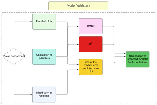
Figure 7.
Flowchart of the model validation.
The residual plot and their distribution are presented in Figure 8.
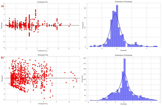
Figure 8.
Residual plot and their distribution: (a) chassis dynamometer data and (b) on-road test.
Figure 8 allows for a preliminary analysis of the regression model errors. The x-axis depicts the model-predicted values, while the y-axis shows the discrepancies between the actual and predicted values, known as residuals. Each point in the plot corresponds to a data sample. The dashed horizontal line represents zero residuals, indicating accurate model predictions. Points above the line indicate overestimated values, whereas those below represent underestimation. Interpreting this graph helps to assess whether the model overlooks patterns or predicts extreme values, which may result in errors. Ideally, the points should evenly scatter around the zero line, indicating a well-fitted model.
Furthermore, Figure 8 includes a histogram showing the frequency of different residual values. The x-axis displays residual values, while the y-axis shows their frequency. The plot includes kernel density estimation (KDE) to visualise the distribution shape. The colours distinguish elements, with blue representing histogram columns. This plot helps to evaluate how residuals distribute around zero and their absolute values. Ideally, residuals should have a symmetric distribution centred around zero, indicating a well-fitted model.
In cases with large data sets, such as those investigated for chassis dynamometer and on-road data, achieving ideal models that oscillate around zero due to CO2 emission parameter dynamics and variability is challenging. Figure 7 reveals some discrepancies in the residual plot and isolated emission cases above 6 g/s. In particular, replicating driving behaviour relative to assumed driving cycles reduces opportunities for diverse emission data. This limitation can lead to estimation errors when using the data for road or simulation purposes.
In the second step of CO2 model validation, the R2 and RMSE indicators were assessed. R2 is a key metric used in regression analysis to evaluate the quality of the fit of the model to the data. It expresses, on a scale from 0 to 1, the degree to which variability in the dependent variable is explained by the regression model [45]. An R2 value of 0 indicates that the model does not explain the variability in the data, while an R2 value of 1 indicates a perfect fit of the model to the data. In the context of scientific research, the R2 coefficient is a significant criterion for evaluating regression models, enabling researchers to understand the extent to which the model can predict the variability in the data. However, it is recommended to use R2 in conjunction with other metrics to obtain a comprehensive assessment of the performance of the regression model. The R2 indicator is calculated on the basis of the formula:
where R2 is the coefficient of determination, SSM is the sum of squares for the model, SST is the sum of squares total, yt is the actual value of the dependent variable, is the predicted values of the dependent variable, is the average value of the actual dependent variable.
The second metric examined was RMSE. RMSE is another important metric used in evaluating regression models. Measure the spread of the predicted values by the model from the actual values of the dependent variables [46]. RMSE is expressed in the same units as the dependent variable, which facilitates the interpretation of its values. The lower the RMSE value, the better the regression model performs in predicting the data. The RMSE value is particularly significant in experimental analysis, where the precise prediction of the values of the dependent variables is crucial to understanding the phenomenon under study. RMSE is calculated based on the following formula:
where n is the number of samples, yt is the forecast, is the observed values.
The results of the evaluation of the CO2 prediction models obtained for CNG-powered vehicles are presented in Table 2.
Table 2.
The results of the validation metrics for the CO2 emission prediction models obtained.
Based on the results presented in Table 2, it can be observed that the model obtained for the chassis dynamometer data exhibits higher R2 and RMSE values for both the test and training data. This may result from the lower variability of these tests due to the controlled conditions in the laboratory. The nature of driving in such tests leads to achieving results within certain ranges of vehicle operation. Consequently, the models derived from such data tend to perform better in terms of metrics. However, when comparing these results to on-road data, it would be challenging for such a model to accurately predict CO2 emissions without significant prediction errors. It is also worth noting here the characteristics of the chassis dynamometer tests themselves; the input cycles for such laboratory tests can be varied by applying different modifications to these driving cycles. On the contrary, the CO2 emission model obtained from on-road data shows lower validation metric values. Nevertheless, it is not always advisable to rely solely on these metrics, especially when dealing with large amounts of data, particularly from dynamic experiments that are difficult to replicate. In the next section, the predictive capabilities of both models will be compared using new on-road data. The road data were chosen because it is the target of future vehicle emission tests and better reflects actual vehicle emissions.
3.4. Example Use and Comparison of the Obtained Models
To evaluate the generated CO2 emission models for a CNG-powered vehicle, another new road test was conducted. Data from this test were used to generate a comparative plot of prediction errors in emissions between model predictions and actual values (Figure 9). Based on Figure 9, it can be observed that the CO2 model created based on the chassis dynamometer data exhibits significantly larger errors. This is largely influenced by the diversity of input data into the model. For a better visualisation of the results obtained by the models, views of CO2 emission maps were also prepared.
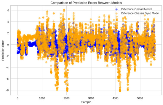
Figure 9.
Differences in CO2 estimation for new road data not previously used.
To accelerate result generation, a preliminary version of the user interface was prepared for the CO2 emission model application for a CNG-powered vehicle. An overview of the application window is depicted in Figure 10. The interface containing the model data was designed using the Python library Tkinter. The Tkinter library is a standard toolkit for creating graphical user interfaces (GUIs) in the Python language [47].
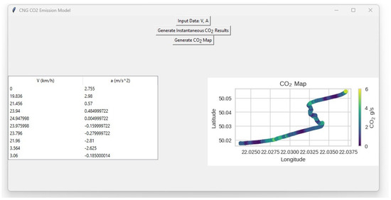
Figure 10.
View of the application window to estimate CO2 from a CNG-fuelled vehicle.
Based on the models and application developed, the comparison of CO2 emission maps for new, unused road data models with models obtained through training using road and chassis dynamometer data are presented in Figure 11 below. All obtained CO2 emission maps were scaled for the range of 0–6 g/s. On the basis of the obtained CO2 emission maps, the following observations can be made:
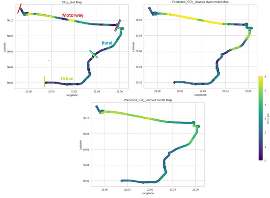
Figure 11.
Maps of CO2 emissions from a CNG-powered vehicle for real and model data—route with an indication of its parts in relation to driving characteristics.
- A significant underestimation of CO2 emissions for the highway section is evident in the model built based on chassis dynamometer data, with a significantly larger area of increased CO2 emissions compared to real data;
- For the urban section, there is much less variation in CO2 emissions, resulting from the prevailing traffic conditions and a lower frequency of dynamic acceleration, translating into low CO2 emissions (up to 3 g/s). These emissions are well-represented in both developed models;
- For the rural section, where higher driving speeds of around 70–100 km/h prevail, it can be seen that the chassis dynamometer model overestimates certain areas for vehicle acceleration compared to real data. In this area, the model developed based on on-road data performs better;
- For the highway section, the CO2 emission results for the chassis dynamometer model exceed 7 g/s, surpassing the actual emissions that occur in reality.
The emission maps presented above provide valuable information for characterising vehicle traffic on a micro-scale, particularly when considering vehicle speed profiles. The obtained models can be freely utilised for input data obtained from the road, for example, through GPS systems or for simulation data. The only input data for the model are the vehicle speed and acceleration, which increases its usability. Analysing vehicle traffic on a microscale and its impact on generated emissions can support certain road modification processes, traffic signal programmes, etc. The aim of such actions may also be to improve traffic flow in certain areas of the city and verify it, for example, through vehicle location data based on emission maps.
4. Discussion
The methodology developed to obtain CO2 emission models provides valuable insights relevant to both the design of such models and their subsequent use. On the basis of the obtained results, it can be observed how crucial the input data are for developing such CO2 emission models. Chassis dynamometer data offer certain possibilities for obtaining a model that, within certain speed ranges for microscale analyses, can provide values of emissions somewhat close to reality. This mainly concerns data for lower speeds, such as urban driving. However, for higher speeds, this model exhibits a considerable underestimation of results, demonstrating significant measurement errors. This situation persists for this model despite its very good specifications regarding validation indicators. The question at this point refers to the intended purposes of this model. If it is intended to be a more universal model that accurately represents real CO2 emissions, especially in dynamic road conditions, then it may not perform well. In such cases, a better solution is the CO2 model created based on road data. The input data for creating this type of model exhibit a very high degree of variability, making such a model more universal and allowing for more accurate predictions.
It is also worth noting that the CO2 emission models developed, according to the available literature, are the first to be described in detail, along with a detailed presentation of the methodology for their creation.
A review of similar work concerns the techniques of creating models rather than the creation of models for CNG-powered vehicles. An example of a study with a similar thematic scope is [48]. In this study, the author introduces a novel approach to estimating CO2 emissions from vehicles using liquefied petroleum gas (LPG). The research focuses on developing microscale CO2 emission models for LPG vehicles, a relatively unexplored area. Using data from road tests employing portable emission measurement systems (PEMS) and onboard diagnostics (OBDII), the authors constructed their model. The results indicate promising precision, suggesting potential applications in analysing continuous CO2 emissions and creating emission maps for urban environmental assessments. The selected gradient-boosting machine learning method yields validation coefficients of the R2 test = 0.61 and the MSE test = 0.77, strengthening the model’s credibility for assessing LPG vehicle emissions.
Another example of a study that also uses artificial intelligence methods for the prediction of CO2 is [49]. This paper investigates CO2 emission modelling using data from the portable emission measurement system (PEMS) and artificial intelligence methods. Start-stop technology has emerged as a common strategy to mitigate the increase in fuel consumption in vehicles. The methodology introduced here outlines the process of measuring and building a computational model for CO2 emissions using artificial intelligence techniques tailored for vehicles equipped with start-stop technology. The model uses data from vehicle speed, vehicle acceleration, and road gradient for the prediction of CO2 emissions. Among the three machine learning techniques analysed, the gradient boosting method demonstrates superior prediction performance. Validation of the developed models employs determination coefficients, mean squared error, and visual evaluation of residual and instantaneous emission plots, as well as CO2 emission maps. These models introduce a novel methodology and offer potential applications for microscale environmental analysis.
The above-mentioned studies concern the use of similar machine learning techniques for modelling, but the difference lies in the fact that the results presented in this study pertain to the use of the Optuna tool, which allows for even more precise creation of CO2 emission models.
Another study addressing the modelling of emissions using artificial intelligence techniques is [50]. In their study, the researchers aim to address the need for precise models of vehicle emissions, particularly focusing on NOx, to assess the impact of road transport on air pollution. Through the application of machine learning techniques on a data set comprising 70 diesel vehicles tested under real-world driving conditions, the study aims to group vehicles with similar emissions profiles and develop models for predicting instantaneous emissions. The analysis, employing dynamic time warping and clustering based on NOx emissions, successfully identified 17 clusters representing 88% of the data set’s trips. Although the grouping effectively grouped vehicles with similar emissions patterns, no significant correlation was found between emissions and vehicle characteristics such as engine size or weight. Evaluating three models for each cluster: lookup table (LT), nonlinear regression (NLR) and neural network multilayer perceptron (MLP), the study indicates that both NLR and MLP models offer accurate predictions of NOx emissions, with relative errors below 20% and average normalised mean squared errors below 0.3. Despite similar performance, neural networks show better adaptability to vehicles that do not fit into specific clusters. The simplicity of the input required for the proposed models, including vehicle speed and acceleration, suggests their immediate utility for policymakers to predict vehicle NOx emissions and implement mitigation strategies effectively. This study confirms the need for creating such models, especially those that require minimal input data and are easily aggregable. In this work, the authors also developed an emissions model based on speed and acceleration data, facilitating its subsequent use and making such a model widely accessible. The use of artificial intelligence for modelling is gaining popularity. In the current literature, similar modelling techniques can also be found in the context of modelling energy consumption by electric vehicles (EVs) [51,52,53,54].
Other studies also mention other studies that generally concern the use of CNG fuel for vehicle propulsion and the impact of this fuel on emissions. One of such studies is [55]. This study investigates the emissions of a passenger car equipped with a spark ignition engine capable of using both compressed natural gas (CNG) and standard gasoline. The results of emissions tests carried out on a chassis dynamometer are discussed within the framework of Euro 6 emissions requirements. The vehicle under examination, equipped with a multi-point gas injection system, remained unchanged and was aligned with Euro 5 standards [56]. The results indicate that when fuelled with CNG, the vehicle meets the Euro 6 [57] emissions limits, although with discernible differences in emissions depending on the fuel type. In particular, carbon dioxide emissions are markedly reduced when the vehicle operates on CNG compared to gasoline, aligning closely with previous research outcomes. This work is also limited to replicating the NEDC cycle. The observed reduction in CO2 emissions aligns with the typical 25% reduction for CNG. Another study on a similar topic on the applicability of CNG as an alternative fuel is [58]. This study examines strategies to improve energy efficiency and reduce CO2 emissions in medium- and heavy-duty spark ignition engines by substituting gasoline fuels with natural gas. Experimental analyses compare the performance of 91RON, 98RON gasoline and natural gas fuels across seven key operating conditions on a multicylinder research engine. Engine mapping with all three fuels is performed, and CO2 emissions are compared during the emission certification test cycle. Findings indicate that the lower carbon content of natural gas contributes significantly to the reduction of CO2 emissions, while the operation of the engine on natural gas improves fuel efficiency by reducing pumping loss and improving idle stability under idle and part load conditions.
The models and applications obtained for microscale tools can be useful for individuals involved in the analysis of road data, including speed, acceleration, and vehicle ecology. They are particularly important in the context of the creation of future propulsion systems. Models of this type of emissions can also be useful to legislators and transportation decision-makers. Using the predictive capabilities of the model, policymakers can make more informed decisions about transportation strategies aimed at reducing CO2 emissions. The model’s ability to accurately predict CO2 emissions under various driving conditions can provide valuable insights into the environmental impact of different transportation policies and initiatives. Furthermore, it can aid in the development of targeted policies and measures tailored to address specific emission hotspots and promote the adoption of cleaner and more sustainable transportation technologies. Overall, the use of the CO2 emission model can significantly contribute to the formulation of effective policies aimed at mitigating the adverse effects of vehicle emissions on urban air quality and public health. Although electromobility is a somewhat distant solution in terms of time perspective, it is also important to explore other alternative solutions in terms of powering conventional internal combustion engines. The research presented in this study confirms that CNG has a significant potential to reduce CO2 emissions, making it an attractive fuel in the global policy context of decarbonising transportation. For the vehicle examined, the average CO2 emissions for gasoline were, on average, 40% higher than for CNG. It is also important to highlight the directions for further research, especially studies on other vehicles, to diversify across different classes. Chassis dynamometer tests should also be diversified to accommodate the new homologation procedure and other driving cycles commonly used on chassis dynamometers.
5. Conclusions
The study demonstrates the process of creating CO2 emission models for a CNG-powered vehicle. Model development is achieved through the application of artificial intelligence methods for CO2 prediction, specifically utilising the XGBoost technique with hyperparameter optimisation. The models were constructed based on input data from two sources: chassis dynamometer and on-road data. The key points of the study are as follows:
- Development of a methodology for creating CO2 emission models for CNG-powered vehicles using two input parameters: speed and acceleration;
- The CO2 emission model developed based on chassis dynamometer data exhibits high validation metrics, with an R2 of 0.87 and an RMSE of 0.55 for test data;
- The CO2 emission model developed based on road data has validation metrics of R2 of 0.67 and RMSE of 0.77;
- Visual verification of the models obtained based on new road tests revealed limited predictive capabilities for the chassis dynamometer-based model, while the model based on on-road data better represents actual emissions.
The CO2 emission models tailored for vehicles powered by CNG are in agreement with global overarching initiatives aimed at mitigating carbon emissions within the transportation sector. Interestingly, vehicles that use CNG propulsion systems exhibit reduced CO2 emissions compared to their conventional counterparts, significantly contributing to the overall goal of reducing greenhouse gas emissions. This paradigm shift in vehicle emissions underscores the importance of incorporating such emission models into future environmental assessments. These assessments are likely to benefit from the comprehensive emission projections provided by these models, enabling a nuanced understanding of the environmental footprint of CNG-powered vehicles. Furthermore, the integration of detailed emission maps derived from these models offers granular insight into emission hotspots, facilitating targeted interventions and policy formulations to effectively address environmental challenges associated with transportation emissions.
The initial CO2 prediction models for CNG-powered vehicles should be expanded in the future with new input data for a larger number of vehicles. Therefore, the developed application can be continuously updated. At present, this represents the primary limitation of the obtained model and also indicates the direction for further work. CNG fuel is characterised by a significant reduction in greenhouse gases, particularly CO2. Therefore, future vehicle designs, excluding alternative electric powertrains, should be based on renewable fuel sources such as CNG.
Funding
This research received no external funding.
Data Availability Statement
Data can be made available to those interested.
Conflicts of Interest
The author declares no conflict of interest.
References
- Li, Z.; Li, Q.; Chen, T. Record-breaking high-temperature outlook for 2023: An assessment based on the China global merged temperature (cmst) dataset. Adv. Atmos. Sci. 2024, 41, 369–376. [Google Scholar] [CrossRef]
- Rantanen, M.; Räisänen, J.; Merikanto, J. A method for estimating the effect of climate change on monthly mean temperatures: September 2023 and other recent record-warm months in Helsinki, Finland. Atmos. Sci. Lett. 2024, e1216. [Google Scholar] [CrossRef]
- Basma, H.; Rodríguez, F. The European Heavy-Duty Vehicle Market until 2040: Analysis of Decarbonization Pathways; International Council on Clean Transportation: Washington, DC, USA, 2023. [Google Scholar]
- Malec, M. The prospects for decarbonisation in the context of reported resources and energy policy goals: The case of Poland. Energy Policy 2022, 161, 112763. [Google Scholar] [CrossRef]
- Ren, L.; Zhou, S.; Peng, T.; Ou, X. A review of CO2 emissions reduction technologies and low-carbon development in the iron and steel industry focusing on China. Renew. Sustain. Energy Rev. 2021, 143, 110846. [Google Scholar] [CrossRef]
- Kinsella, L.; Stefaniec, A.; Foley, A.; Caulfield, B. Pathways to decarbonising the transport sector: The impacts of electrifying taxi fleets. Renew. Sustain. Energy Rev. 2023, 174, 113160. [Google Scholar] [CrossRef]
- Leroutier, M.; Quirion, P. Air pollution and CO2 from daily mobility: Who emits and Why? Evidence from Paris. Energy Econ. 2022, 109, 105941. [Google Scholar] [CrossRef]
- Krause, J.; Thiel, C.; Tsokolis, D.; Samaras, Z.; Rota, C.; Ward, A.; Prenninger, P.; Coosemans, T.; Neugebauer, S.; Verhoeve, W. EU road vehicle energy consumption and CO2 emissions by 2050–Expert-based scenarios. Energy Policy 2020, 138, 111224. [Google Scholar] [CrossRef]
- Giechaskiel, B.; Valverde, V.; Kontses, A.; Suarez-Bertoa, R.; Selleri, T.; Melas, A.; Otura, M.; Ferrarese, C.; Martini, G.; Balazs, A.; et al. Effect of extreme temperatures and driving conditions on gaseous pollutants of a Euro 6d-Temp gasoline vehicle. Atmosphere 2021, 12, 1011. [Google Scholar] [CrossRef]
- Ziółkowski, A.; Fuć, P.; Jagielski, A.; Bednarek, M.; Konieczka, S. Comparison of the Energy Consumption and Exhaust Emissions between Hybrid and Conventional Vehicles, as Well as Electric Vehicles Fitted with a Range Extender. Energies 2023, 16, 4669. [Google Scholar] [CrossRef]
- Tarei, P.K.; Chand, P.; Gupta, H. Barriers to the adoption of electric vehicles: Evidence from India. J. Clean. Prod. 2021, 291, 125847. [Google Scholar] [CrossRef]
- Adhikari, M.; Ghimire, L.P.; Kim, Y.; Aryal, P.; Khadka, S.B. Identification and analysis of barriers against electric vehicle use. Sustainability 2020, 12, 4850. [Google Scholar] [CrossRef]
- Kuszewski, H.; Jaworski, A.; Mądziel, M.; Woś, P. The investigation of auto-ignition properties of 1-butanol–biodiesel blends under various temperatures conditions. Fuel 2023, 346, 128388. [Google Scholar] [CrossRef]
- Kuszewski, H.; Jaworski, A.; Mądziel, M. Lubricity of Ethanol–Diesel Fuel Blends—Study with the Four-Ball Machine Method. Materials 2021, 14, 2492. [Google Scholar] [CrossRef] [PubMed]
- Lejda, K.; Jaworski, A.; Mądziel, M.; Balawender, K.; Ustrzycki, A.; Savostin-Kosiak, D. Assessment of Petrol and Natural Gas Vehicle Carbon Oxides Emissions in the Laboratory and On-Road Tests. Energies 2021, 14, 1631. [Google Scholar] [CrossRef]
- Aba, M.M.; Amado, N.B.; Rodrigues, A.L.; Sauer, I.L.; Richardson, A.A.M. Energy transition pathways for the Nigerian Road Transport: Implication for energy carrier, Powertrain technology, and CO2 emission. Sustain. Prod. Consum. 2023, 38, 55–68. [Google Scholar] [CrossRef]
- Toumasatos, Z.; Kontses, A.; Doulgeris, S.; Samaras, Z.; Ntziachristos, L. Particle emissions measurements on CNG vehicles focusing on Sub-23nm. Aerosol Sci. Technol. 2021, 55, 182–193. [Google Scholar] [CrossRef]
- Shamsapour, N.; Hajinezhad, A.; Noorollahi, Y. Developing a system dynamics approach for CNG vehicles for low-carbon urban transport: A case study. Int. J. Low-Carbon Technol. 2021, 16, 577–591. [Google Scholar] [CrossRef]
- McCaffery, C.; Zhu, H.; Tang, T.; Li, C.; Karavalakis, G.; Cao, S.; Oshinuga, A.; Burnette, A.; Johnson, K.C.; Durbin, T.D. Real-world NOx emissions from heavy-duty diesel, natural gas, and diesel hybrid electric vehicles of different vocations on California roadways. Sci. Total Environ. 2021, 784, 147224. [Google Scholar] [CrossRef]
- Mac Kinnon, M.; Zhu, S.; Cervantes, A.; Dabdub, D.; Samuelsen, G.S. Benefits of near-zero freight: The air quality and health impacts of low-NOx compressed natural gas trucks. J. Air Waste Manag. Assoc. 2021, 71, 1428–1444. [Google Scholar] [CrossRef]
- Ryan, F.; Caulfield, B. Examining the benefits of using bio-CNG in urban bus operations. Transp. Res. Part D Transp. Environ. 2010, 15, 362–365. [Google Scholar] [CrossRef]
- Gnann, T.; Speth, D.; Seddig, K.; Stich, M.; Schade, W.; Vilchez, J.G. How to integrate real-world user behavior into models of the market diffusion of alternative fuels in passenger cars-An in-depth comparison of three models for Germany. Renew. Sustain. Energy Rev. 2022, 158, 112103. [Google Scholar] [CrossRef]
- Dixit, S.; Ramachandra Rao, K.; Tiwari, G.; von Wieding, S. Urban freight characteristics and externalities–A comparative study of Gothenburg (Sweden) and Delhi (India). J. Transp. Supply Chain Manag. 2022, 16, 629. [Google Scholar] [CrossRef]
- Quintili, A.; Castellani, B. The energy and carbon footprint of an urban waste collection fleet: A case study in central Italy. Recycling 2020, 5, 25. [Google Scholar] [CrossRef]
- Burchart-Korol, D.; Gazda-Grzywacz, M.; Zarębska, K. Research and prospects for the development of alternative fuels in the transport sector in Poland: A review. Energies 2020, 13, 2988. [Google Scholar] [CrossRef]
- Górniak, A.; Midor, K.; Kaźmierczak, J.; Kaniak, W. Advantages and disadvantages of using methane from CNG in motor vehicles in polish conditions. Multidiscip. Asp. Prod. Eng. 2018, 1, 241–247. [Google Scholar] [CrossRef][Green Version]
- Kowalska-Pyzalska, A.; Kott, J.; Kott, M. Why Polish market of alternative fuel vehicles (AFVs) is the smallest in Europe? SWOT analysis of opportunities and threats. Renew. Sustain. Energy Rev. 2020, 133, 110076. [Google Scholar] [CrossRef]
- Mądziel, M. Vehicle Emission Models and Traffic Simulators: A Review. Energies 2023, 16, 3941. [Google Scholar] [CrossRef]
- Andrych-Zalewska, M.; Chlopek, Z.; Pielecha, J.; Merkisz, J. Investigation of exhaust emissions from the gasoline engine of a light duty vehicle in the Real Driving Emissions test. Eksploat. Niezawodn. 2023, 25, 165880. [Google Scholar] [CrossRef]
- Rymaniak, Ł.; Merkisz, J.; Szymlet, N.; Kamińska, M.; Weymann, S. Use of emission indicators related to CO2 emissions in the ecological assessment of an agricultural tractor. Eksploat. Niezawodn. 2021, 23, 605–611. [Google Scholar] [CrossRef]
- Sathish, T.; Muthulakshmanan, A. Modelling of Manhattan K-nearest neighbor for exhaust emission analysis of CNG-diesel engine. J. Appl. Fluid Mech. 2018, 11, 39–44. [Google Scholar]
- Rahman, M.M.; Zhou, Y.; Rogers, J.; Chen, V.; Sattler, M.; Hyun, K. A comparative assessment of CO2 emission between gasoline, electric, and hybrid vehicles: A Well-To-Wheel perspective using agent-based modeling. J. Clean. Prod. 2021, 321, 128931. [Google Scholar] [CrossRef]
- Wei, T.; Frey, H.C. Evaluation of the precision and accuracy of cycle-average light duty gasoline vehicles tailpipe emission rates predicted by modal models. Transp. Res. Rec. 2020, 2674, 566–584. [Google Scholar] [CrossRef]
- Wei, N.; Zhang, Q.; Zhang, Y.; Jin, J.; Chang, J.; Yang, Z.; Ma, C.; Jia, Z.; Ren, C.; Wu, L. Super-learner model realizes the transient prediction of CO2 and NOx of diesel trucks: Model development, evaluation and interpretation. Environ. Int. 2022, 158, 106977. [Google Scholar] [CrossRef] [PubMed]
- Seo, J.; Yun, B.; Park, J.; Park, J.; Shin, M.; Park, S. Prediction of instantaneous real-world emissions from diesel light-duty vehicles based on an integrated artificial neural network and vehicle dynamics model. Sci. Total Environ. 2021, 786, 147359. [Google Scholar] [CrossRef] [PubMed]
- Wang, X.; Chen, L.W.; Lu, M.; Ho, K.F.; Lee, S.C.; Ho, S.S.; Chow, J.C.; Watson, J.G. Apportionment of vehicle fleet emissions by linear regression, positive matrix factorization, and emission modeling. Atmosphere 2022, 13, 1066. [Google Scholar] [CrossRef]
- Ning, Z.; Chan, T.L. On-road remote sensing of liquefied petroleum gas (LPG) vehicle emissions measurement and emission factors estimation. Atmos. Environ. 2007, 41, 9099–9110. [Google Scholar] [CrossRef]
- Mądziel, M. Future Cities Carbon Emission Models: Hybrid Vehicle Emission Modelling for Low-Emission Zones. Energies 2023, 16, 6928. [Google Scholar] [CrossRef]
- Lijewski, P.; Merkisz, J.; Fuć, P.; Ziółkowski, A.; Rymaniak, Ł.; Kusiak, W. Fuel consumption and exhaust emissions in the process of mechanized timber extraction and transport. Eur. J. For. Res. 2017, 136, 153–160. [Google Scholar] [CrossRef]
- Chen, T.; He, T.; Benesty, M.; Khotilovich, V.; Tang, Y.; Cho, H.; Chen, K.; Mitchell, R.; Cano, I.; Zhou, T. Xgboost: Extreme Gradient Boosting, R Package Version 0.4-2. 2015. Available online: https://www.rdocumentation.org/packages/xgboost/versions/0.4-2 (accessed on 1 March 2024).
- DR, U.S.; Patil, A.; Mohana. Malicious URL Detection and Classification Analysis using Machine Learning Models. In Proceedings of the 2023 International Conference on Intelligent Data Communication Technologies and Internet of Things (IDCIoT), Bengaluru, India, 5–7 January 2023; pp. 470–476. [Google Scholar]
- Sulzer, V.; Marquis, S.G.; Timms, R.; Robinson, M.; Chapman, S.J. Python battery mathematical modelling (PyBaMM). J. Open Res. Softw. 2021, 9, 14. [Google Scholar] [CrossRef]
- Molner, A.; Carrillo-Perez, F.; Guillén, A. SnapperML: A python-based framework to improve machine learning operations. SoftwareX 2024, 26, 101648. [Google Scholar] [CrossRef]
- Akiba, T.; Sano, S.; Yanase, T.; Ohta, T.; Koyama, M. Optuna: A next-generation hyperparameter optimization framework. In Proceedings of the 25th ACM SIGKDD International Conference on Knowledge Discovery & Data Mining, Anchorage, AK, USA, 4–8 August 2019; pp. 2623–2631. [Google Scholar]
- Lüdecke, D.; Ben-Shachar, M.S.; Patil, I.; Waggoner, P.; Makowski, D. Performance: An R package for assessment, comparison and testing of statistical models. J. Open Source Softw. 2021, 6, 3139. [Google Scholar] [CrossRef]
- Hodson, T.O. Root mean square error (RMSE) or mean absolute error (MAE): When to use them or not. Geosci. Model Dev. Discuss. 2022, 15, 5481–5487. [Google Scholar] [CrossRef]
- Amos, D. Python Gui Programming with Tkinter. 2020. 71. Available online: https://realpython.com/python-gui-tkinter (accessed on 1 March 2024).
- Mądziel, M. Liquified Petroleum Gas-Fuelled Vehicle CO2 Emission Modelling Based on Portable Emission Measurement System, On-Board Diagnostics Data, and Gradient-Boosting Machine Learning. Energies 2023, 16, 2754. [Google Scholar] [CrossRef]
- Mądziel, M. Instantaneous CO2 emission modelling for a Euro 6 start-stop vehicle based on portable emission measurement system data and artificial intelligence methods. Environ. Sci. Pollut. Res. 2024, 31, 6944–6959. [Google Scholar] [CrossRef] [PubMed]
- Le Cornec, C.M.; Molden, N.; van Reeuwijk, M.; Stettler, M.E. Modelling of instantaneous emissions from diesel vehicles with a special focus on NOx: Insights from machine learning techniques. Sci. Total Environ. 2020, 737, 139625. [Google Scholar] [CrossRef] [PubMed]
- Zhang, Q.; Tian, S.; Lin, X. Recent advances and applications of ai-based mathematical modeling in predictive control of hybrid electric vehicle energy management in china. Electronics 2023, 12, 445. [Google Scholar] [CrossRef]
- Mądziel, M. Energy Modeling for Electric Vehicles Based on Real Driving Cycles: An Artificial Intelligence Approach for Microscale Analyses. Energies 2024, 17, 1148. [Google Scholar] [CrossRef]
- Wei, H.; Ai, Q.; Zhao, W.; Zhang, Y. Modelling and experimental validation of an EV torque distribution strategy towards active safety and energy efficiency. Energy 2022, 239, 121953. [Google Scholar] [CrossRef]
- Mathankumar, M.; Gunapriya, B.; Guru, R.R.; Singaravelan, A.; Sanjeevikumar, P. AI and ML powered IoT applications for energy management in electric vehicles. Wireless Pers. Commun. 2022, 126, 1223–1239. [Google Scholar] [CrossRef]
- Bielaczyc, P.; Woodburn, J.; Szczotka, A. An assessment of regulated emissions and CO2 emissions from a European light-duty CNG-fueled vehicle in the context of Euro 6 emissions regulations. Appl. Energy 2014, 117, 134–141. [Google Scholar] [CrossRef]
- Regulation (EC) No 715/2007 of the European Parliament and of the Council of 20 June 2007 on Type Approval of Motor Vehicles with Respect to Emissions from Light Passenger and Commercial Vehicles (Euro 5 and Euro 6) and on Access to Vehicle Repair and Maintenance Information. Available online: https://eur-lex.europa.eu/eli/reg/2007/715/oj (accessed on 2 February 2024).
- Commission Regulation (EU) No 459/2012 of 29 May 2012 amending Regulation (EC) No 715/2007 of the European Parliament and of the Council and Commission Regulation (EC) No 692/2008 as Regards Emissions from Light Passenger and Commercial Vehicles (Euro 6). Available online: https://eur-lex.europa.eu/LexUriServ/LexUriServ.do?uri=OJ:L:2012:142:0016:0024:en:PDF (accessed on 2 February 2024).
- Divekar, P.; Han, X.; Zhang, X.; Zheng, M.; Tjong, J. Energy efficiency improvements and CO2 emission reduction by CNG use in medium-and heavy-duty spark-ignition engines. Energy 2023, 263, 125769. [Google Scholar] [CrossRef]


Disclaimer/Publisher’s Note: The statements, opinions and data contained in all publications are solely those of the individual author(s) and contributor(s) and not of MDPI and/or the editor(s). MDPI and/or the editor(s) disclaim responsibility for any injury to people or property resulting from any ideas, methods, instructions or products referred to in the content. |
© 2024 by the author. Licensee MDPI, Basel, Switzerland. This article is an open access article distributed under the terms and conditions of the Creative Commons Attribution (CC BY) license (https://creativecommons.org/licenses/by/4.0/).