Outlook for Offshore Wind Energy Development in Mexico from WRF Simulations and CMIP6 Projections

Abstract

This study presents a comprehensive assessment of the offshore wind energy potential in Mexico across 40 years (1979–2018) of numerical simulations using the Weather Research and Forecasting (WRF) model and data from the Coupled Model Intercomparison Project Phase 6 (CMIP6). The WRF identifies three regions with moderate to good wind potential: off the north coast of Tamaulipas (Zone I), the northwest coast of Yucatan (Zone II), and the Gulf of Tehuantepec (Zone III). The analysis involves comparing 47 CMIP6 climate models with the WRF results and selecting the best performing models to obtain future projections for the short term (2040–2069) and the long term (2070–2099). Two ensemble-based strategies were implemented. The first one, which uses an intersection approach from which four CMIP6 models were considered, reveals positive percentage differences in Zone II for both future projections, especially for the long-term one. In Zones I and III, positive values are also observed near the coast, mainly for the long-term projection, but they are considerably lower compared to those in Zone II. The second ensemble strategy uses weight assignment through the Mean Absolute Percentage Error, so that a greater weight is given to the model that performed better in each particular zone, potentially providing more accurate results. The findings suggest the likelihood of increased offshore wind energy in these three zones of Mexico, for both short- and long-term future projections, with positive percentage differences of up to 10% in certain areas.

1. Introduction

Wind energy is a promising solution to mitigate the effects of climate change, as it is considered to be a clean and renewable energy source that does not emit greenhouse gasses during plant operation. Although, it must be taken into account that any generation facility has a carbon footprint that has to consider prospection, design, materials extraction, transportation, manufacturing, and decommissioning, among other factors. In energy production, when comparing various sources, there is a stark contrast in the amount of greenhouse gas emissions. Wind power, for instance, emits just 11 g of CO₂ per kWh, significantly less than coal, which generates a staggering 980 g of CO₂ per kWh, and natural gas, which emits about 465 g of CO₂ per kWh [1]. However, the development of wind energy is not without challenges: social, economic, political, technical, and environmental factors may limit its growth [2]. In particular, offshore wind energy projects require significant investment in infrastructure, technology, and labor, although this can stimulate economic growth in the regions where they are developed. Potential impacts on marine ecosystems, such as seabirds, marine mammals, and fish populations, include collision risks, habitat alteration, and acoustic disturbances. To minimize these impacts, it is crucial to take advantage of technological advances and implement noise reduction measures, as well as find adequate locations and management for offshore wind farms [3,4]. Additionally, there may be visual and aesthetic impacts on coastal areas and seascapes, which communities may perceive positively or negatively depending on individual preferences and cultural values [5].

Despite these challenges, the global wind power market is expected to experience significant growth in the short term driven by the increasing energy demand. Due to the advantages of energy generation in offshore wind farms compared to that onshore, which are related to greater wind intensity and more persistent winds over the ocean surface, significant investments have recently been made in these types of facilities. For example, in Europe, offshore wind power accounted for 13% of new installations in 2022, connecting 2.5 GW of wind capacity to the grid. The United Kingdom ranked at the top of the list with 1.2 GW, followed by France (0.5 GW), the Netherlands (0.4 GW), and Germany (0.3 GW) [6].

In this context, Mexico is faced with the imperative challenge of breaking free from its entrenched reliance on fossil fuels and embracing a more ambitious approach toward renewable energy. Achieving this requires the implementation of decisive energy policies, the removal of barriers, the development of the capacities of renewable technologies, and a new energy culture within society [7]. Only through a collective and sustained endeavor can the nation fully harness the vast potential of renewable energies, thus propelling Mexico towards a more sustainable and resilient energy future [7]. According to a progress report on clean energy in Mexico, the country generated 86.27 TWh of clean energy in 2021, accounting for 26.7% of the total, which falls short of the 35% goal set by Mexico in the Energy Transition Law [8]. Additionally, Mexico has a large wind capacity potential, estimated at 3669 GW, but the accumulated installed capacity at the end of 2021 was only 7154 MW [8].

Some previous studies have recognized Mexico’s potential for offshore wind energy development. In particular, Canul-Reyes et al. [9] identified two areas with high wind energy potential in Mexico using the ERA5 and MERRA-2 reanalyses: northeast Tamaulipas and the northwest Yucatan Peninsula. These findings were supported by Arenas-Lopez and Badaoui [10], who assessed wind resource potential in coastal Mexico using 40 years of MERRA-2 data and identified several areas with high wind power density, including Tamaulipas. Furthermore, Bernal-Camacho et al. [11] evaluated the technical feasibility of using floating offshore wind turbines in the Gulf of Tehuantepec, and recommended safety and stabilization measures during extreme conditions. These studies have outlined an initial depiction of the offshore wind resource in Mexico, but it is necessary to carry out a comprehensive climatological analysis that incorporates the behavior of the wind in the coming decades, given the challenges imposed by climate change.

Research carried out in different places worldwide has been based on data from the sixth phase of the Coupled Model Intercomparison Project (CMIP6) to project continental and marine wind resources under future scenarios defined by the Intergovernmental Panel on Climate Change (IPCC). Among them, Martinez and Iglesias [12,13] applied a novel multi-model downscaling approach to CMIP6 projections from an 18-model global climate ensemble. They compared evolving wind resources under climate scenarios across 11 European regions [12], and at national/sub-national scales in Canada, the U.S., Mexico, and Central America [13], generating wind projections under two Shared Socioeconomic Pathways (SSP), the SSP2-4.5 (moderate emissions) and SSP5-8.5 (intensive emissions) (see Section 2.2 below). For Mexico, Martinez and Iglesias [10] anticipate increases in wind power density, mainly in the long-term future (2091–2100), specifically for regions in the northeast and south of Mexico. Shen et al. [14] evaluated the ability of CMIP6 models to simulate long-term surface wind changes. They projected decreases in average global wind speeds, but showed variations between regions which they attributed to asymmetric changes between the hemispheres arising from changes in the surface air temperature gradient caused by increasing greenhouse gas emissions over time. Furthermore, Zhang et al. [15] projected offshore wind energy impacts in China for the period 2021–2100 using CMIP6 models and a downscaling method based on deep learning networks. The authors identified small decreases over the East China Sea and increases in the South China Sea under the same scenarios mentioned above.

Previous studies related to the estimation of future projections of wind resources have not specifically addressed the marine regions in Mexico that could have promising climate prospects within this clean energy sector. Therefore, the motivation for this research arises from the absence of a comprehensive climatological analysis of the offshore wind resources in Mexico, including climate projections. Our approach to addressing this gap involves using high-resolution numerical simulations generated with the Weather Research and Forecasting model (WRF) to characterize historical climatology and leveraging results from the CMIP6 models to obtain future projections. Likewise, we review different technological and terrain features to analyze the viability of operating offshore wind farms in different marine areas of Mexico, in order to support decision making and industry growth.

Overall, this work encompasses the following main aspects:

• Identification of marine regions in Mexico with significant wind energy potential using 40 years of high spatial resolution numerical simulations with the WRF model.
• Evaluation of the feasibility of developing offshore wind farms in these regions based on the analysis of bathymetric data and the availability of nearby transmission lines.
• Assessment of the ability of the CMIP6 models to reproduce the climatic characteristics of the wind field in the identified regions. This evaluation is conducted by comparing CMIP6 data with the monthly climatologies of wind magnitude obtained from the WRF simulations.
• Obtaining future projections for the regions in Mexico with high offshore wind potential from the results provided by the CMIP6 models that exhibited the best performance. In this study, data from the SSP5-8.5 scenario, representing the most severe future climate projection, are analyzed.

A feature that distinguishes our study from previous work is the use of relatively high-resolution (~10 km) numerical simulations with the WRF model, which provide more detailed results compared to the data sources used in similar previous studies and to global climate models. Also, a novel idea is the generation of ensembles considering only those CMIP6 models that showed a good performance in reproducing the magnitude of the winds in the areas of interest, instead of using all available models.

A description of the data sources, including WRF model configuration and CMIP6 models, handling, and processing is presented in Section 2. The Section 3 begins with the identification of areas with high/moderate offshore wind potential in Mexico, followed by a description of their bathymetric features and the availability of nearby transmission lines. Next, a comparative analysis between the WRF simulations and the CMIP6 models is presented for the average wind speed at 50 m above the surface in the identified marine areas. At the end of the Section 3, the construction of ensembles with different CMIP6 models for each region is presented and the future projections of wind energy are analyzed. The Section 4 aims to summarize the main results of the study and to present a discussion of them. Finally, the conclusions of the research are presented in the Section 5 of the manuscript.

2. Data and Methods

2.1. WRF Simulations

The Weather Research and Forecasting (WRF) model was developed through the collaboration of research institutions led by the National Center for Atmospheric Research (NCAR) [16]. As one of the most widely used regional climate models, WRF is a flexible and customizable model that can be adapted to different applications such as weather forecasting, air quality assessment, and renewable energy evaluation. Its dynamic core is a numerical scheme that solves the governing equations of fluid motion, and it also has a set of parameterization schemes that represent physical processes such as boundary layer interactions, convection, and radiation, among others.

WRF applications range from regional to micro scales, and allow for an evaluation of the impact of various factors, such as terrain [17], land use [18,19], and atmospheric stability [20]. WRF has been applied in the assessment of wind energy potential, including in the European Wind Atlas project which aimed to create a high-resolution, high-quality wind resource atlas [21,22,23]. Completed in 2014, the atlas provided valuable information to the wind industry and policymakers for the siting, design optimization, and planning of wind turbines and farms [23]. WRF was also used to reconstruct wind speeds in the Taiwan Strait in the period 1981–2000, establishing a baseline for the region from which the potential influence of climate change on regional wind patterns was evaluated through a statistical downscaling framework applied to the outputs of some CMIP6 models [24].

In the specific case of Mexico, the Ocean-Atmosphere Interaction Group (IOA) [25] of the Institute of Atmospheric Sciences and Climate Change (ICAyCC) [26] at the National Autonomous University of Mexico (UNAM) has employed the WRF model [16] to generate a 40-year hindcast (1979–2018) that serves as a baseline for climate studies in Mexico and its maritime zones. The IOA group has used the WRF model in several research areas, such as incorporating accurate land cover data into atmospheric modeling to improve regional climate simulation and weather forecast accuracy [27,28]. They have also studied the sensitivity of the WRF model to different initial and boundary conditions of the Global Forecast System model at various resolutions [29], analyzed the model’s performance in capturing the dynamics of sea breezes and their interactions with other meteorological phenomena [30], and evaluated the model’s sensitivity to different Land Surface Models (LSMs) to reproduce surface temperature variations in Mexico [31].

The WRF simulations used in this study were conducted using version 3.9.1, with a horizontal resolution of 10 km, 50 vertical levels, and an hourly temporal resolution. The initial and boundary conditions are from the Climate Forecast System Reanalysis (CFSR) dataset [32], which provides global atmospheric and land surface fields at a horizontal resolution of 0.5° and 37 pressure levels. The domain of the simulations covers a wide geographic area, ranging from 5.08° N to 35.73° N and from 70.51° W to 129.48° W. The simulations were run on the Miztli supercomputer at UNAM, requiring approximately 11,000 h of computing time [33].

Table 1. Weather Research and Forecasting (WRF) physics parameterization schemes.

Parameterization Scheme	Scheme Used
Land Surface Model	Noah-MP
Surface Layer Model	MM5 Monin-Obukhov
Microphysics	WRF Single-moment 3-class
Shortwave Radiation	Dudhia Shortwave Scheme
Longwave Radiation	RRTM Longwave Scheme
Planetary Boundary Layer	Yonsei University Scheme (YSU)
Convection	Kain-Fritsch Scheme

provides information on the WRF physics parameterization schemes employed.

To carry out the processing of the large volume of data from the 40-year WRF simulations (1979–2018), a high-performance computing (HPC) cluster was used, dedicated to the development of numerical weather prediction models and the execution of operational forecasting at the ICAyCC-UNAM. This cluster offers a significant computational capacity, with 1360 cores and a combined processing power of 42 Tflops, as well as a large storage capacity of over 700 TB.

To have a more adequate representation of land use and land cover (LULC) for Mexico, a high-resolution database was incorporated based on information from the National Institute of Statistics and Geography (INEGI) of Mexico (López-Espinoza et al. [27] and Rivera-Martínez [28]). In addition, Meza-Carreto [31] found that, for most of Mexico, the Noah-MP LSM scheme provided a better representation of temperature variability. Consequently, this scheme is the one used for the WRF simulations. In particular, the LULC data set used in the WRF hindcast is more complete and accurate than the predetermined global information. This is very important since this information has a direct effect on the LSM scheme and, therefore, also on the PBL scheme of the WRF model; that is, it has a significant influence on the modeling of the processes that occur at the surface–atmosphere interface, as well as in the structure of the atmospheric boundary layer [34]. Figure 1 shows the LULC classifications from INEGI and the USGS [35] and the non-match map between both classifications, where it can be seen that there are no coincidences in large parts of the Mexican territory.

2.2. CMIP6 Models

The CMIP6 project is a coordinated international effort organized by the WCRP (World Climate Research Programme) and the CMA (Climate Modeling Alliance) to provide a comprehensive set of coupled climate model simulations using advanced models [36,37,38,39]. Its main goal is to improve our understanding of the Earth’s climate system and its response to anthropogenic and natural forcings, including the evaluation of future climate projections. CMIP6 includes various institution/country models to allow direct comparisons of performance and structural differences [40,41].

CMIP6 uses updated Global Circulation Models (GCMs) driven by a new set of emissions and land use scenarios, as described in Riahi et al. [42], and encompasses historical (1850–2014) and climate projection (2015–2100) experiments. Historical simulations bridge the gap between past and present by utilizing modern climate observations. Climate projections are provided by the Scenario Model Intercomparison Project (Scenario-MIP), the main activity within the CMIP6. They cover the period from 2015 to 2100, and are based on the Shared Socioeconomic Pathways (SSPs) and the Representative Concentration Pathways, which reflect different possible future trajectories of societal development, including economic growth, energy use, land use, and population growth, among others.

The SSP5-8.5 scenario used in this study is one of eight scenarios developed within the SSP framework, which links socioeconomic scenarios to greenhouse gas emissions trajectories. SSP5-8.5 projects a radiative forcing of 8.5 W m⁻² by the end of the 21st century, estimated by integrated assessment models [43]. This scenario is characterized by heavy reliance on fossil fuels for economic growth and assumes no additional mitigation policies, resulting in a substantial increase in greenhouse gas emissions; it also plays a crucial role in climate research by assessing the potential impacts of high emissions pathways on various Earth system components, such as temperature rise, precipitation patterns, sea level rise, and ecosystem changes.

Data are provided on a regular global grid, with the horizontal resolution varying between models and vertical coverage including levels from 1 to 1000 hPa.

Table 2. Models within the Coupled Model Intercomparison Project Phase 6 (CMIP6).

Modeling Center/Nation	Model Name	Horizontal Resolution
Commonwealth Scientific and Industrial Research Organization/Australia	access_cm2, access_esm1_5	1.25° × 1.875°, 1.25° × 1.875°
Alfred Wegener Institute, Helmholtz Centre for Polar and Marine Research/Germany	awi_cm_1_1_mr, awi_esm_1_1_lr	0.94° × 0.94°, 1.8° × 1.8°
Beijing Climate Center China Meteorological Administration/China	bcc_csm2_mr, bcc_esm1	1.125° × 1.125°, 2.81° × 2.81°
Canadian Centre for Climate Modelling and Analysis/Canada	canesm5_canoe	2.8° × 2.8°
National Center for Atmospheric Research, Climate and Global Dynamics Laboratory/USA	cesm2, cesm2_fv2, cesm2_waccm, cesm2_waccm_fv2	0.94° × 1.25°, 2.5° × 1.8°, 0.94° × 1.25°, 2.5° × 1.8°
Fondazione Centro Euro-Mediterraneo sui Cambiamenti Climatici/Italy	cmcc_cm2_hr4, cmcc_cm2_sr5, cmcc_esm2	0.94° × 0.94°, 0.94° × 0.94°, 0.94° × 0.94°
Centre National de Recherches Météorologiques–Centre Européen de Recherche et de Formation Avancée en Calcul Scientifique/France	cnrm_cm6_1, cnrm_cm6_1_hr, cnrm_esm2_1	1.4° × 1.4°, 0.50° × 0.50°, 1.4° × 1.4°
LLNL (Lawrence Livermore National Laboratory, Livermore, CA 94550, USA); ANL (Argonne National Laboratory, Argonne, IL 60439, USA); BNL (Brookhaven National Laboratory, Upton, NY 11973, USA); LANL (Los Alamos National Laboratory, Los Alamos, NM 87545, USA); LBNL (Lawrence Berkeley National Laboratory, Berkeley, CA 94720, USA); ORNL (Oak Ridge National Laboratory, Oak Ridge, TN 37831, USA); PNNL (Pacific Northwest National Laboratory, Richland, WA 99352, USA); SNL (Sandia National Laboratories, Albuquerque, NM 87185, USA)	e3sm_1_0, e3sm_1_1, e3sm_1_1_eca	0.94° × 0.94°, 0.94° × 0.94°, 1.25° × 1.875°
Fondazione Centro Euro-Mediterraneo sui Cambiamenti Climatici/Italy	fgoals_f3_l	1.125° × 1.125°
Geophysical Fluid Dynamics Laboratory/USA	fgoals_g3	2.5° × 1.875°
Geophysical Fluid Dynamics Laboratory/USA	gfdl_esm4	0.94° × 0.94°
German Climate Computing Center/Germany	hadgem3_gc31_ll, hadgem3_gc31_mm	2.5° × 2.5°, 2.5° × 2.5°
Institute for Global Environmental Strategies/Japan	inm_cm4_8, inm_cm5_0	2.0° × 2.5°, 2.0° × 2.5°
Institute of Numerical Mathematics, Russian Academy of Sciences/Russia	iitm_esm	0.94° × 0.94°
Institut Pierre-Simon Laplace/France	ipsl_cm5a2_inca, ipsl_cm6a_lr	1.4° × 1.4°, 1.4° × 1.4°
Japan Agency for Marine-Earth Science and Technology/Japan	kace_1_0_g	1.125° × 1.125°
Korea Institute of Ocean Science and Technology/South Korea	kiost_esm	1.5° × 1.5°
Max Planck Institute for Meteorology/Germany	mpi_esm1_2_hr, mpi_esm1_2_lr	0.94° × 0.94°, 0.94° × 0.94°
Meteorological Research Institute/Japan	mri_esm2_0	0.94° × 0.94°
Norwegian Computing Center/Norway	noresm2_lm, noresm2_mm	1.25° × 1.875°, 1.25° × 1.875°
Research Institute for Global Change/Japan	sam0_unicon	1.25° × 1.875°
The Australian National University/Australia	taiesm1	1.875° × 3.75°
National Institute for Environmental Studies/Japan	ukesm1_0_ll	2.5° × 2.5°
European consortium of national meteorological services and research institutes	EC-Earth3, EC-Earth3-Veg, EC-Earth3-AerChem, EC-Earth3-CC	0.94° × 0.94°, 0.94° × 0.94°, 0.94° × 0.94°, 0.94° × 0.94°
First Institute of Oceanography, State Oceanic Administration, Qingdao National Laboratory for Marine Science and Technology/China	fio_esm_2_0	0.94° × 0.94°

includes a list of the CMIP6 models, along with their name, origin, and spatial resolution. To acquire the CMIP6 data, the Python CDSAPI library (version 0.6.1) was used [44], which allows for easy access to and retrieval of data from the Copernicus Climate Data Store. Data are available at monthly, daily, and fixed temporal resolutions, and the format follows the NetCDF4 standard.

The monthly near-surface wind speed data from 47 available models were downloaded for the historical period of 1985–2014, as well as for the future projections of 2040–2069 and 2070–2099. The choice of the historical period from 1985 to 2014 is based on the availability of climate data from CMIP6 models, which cover the most recent 30 years up to the cutoff date in 2014. This time window provides a robust foundation for assessing projected changes in the future. Furthermore, the selection of 30-year periods for future projections, specifically 2040–2069 and 2070–2099, was made to maintain consistency in the duration of the analyses and ensure comparability between historical and future results.

2.3. Methods

2.3.1. Regridding CMIP6 Data to the WRF Grid

In this study, we employed the regridding process to interpolate the CMIP6 data to the fixed grid of the WRF model. The CMIP6 models have different grid configurations, while the WRF model has a resolution of 10 km. Regridding allows us to transform the CMIP6 data from its original grid representation to its corresponding position in the WRF grid in a systematic manner. To achieve accurate regridding, the new capabilities available in NCL were utilized, employing the Earth System Modeling Framework software (version 6.6.2) [45], which provides advanced regridding techniques that are compatible with rectilinear, curvilinear, and unstructured grids. In this study, the bilinear interpolation method was employed, preserving the linearity and smoothness of the data during the regridding process.

2.3.2. Application of the Power Law Method

In order to estimate wind speed at various heights, the power law method was used, which is a widely used technique in wind energy studies [46,47]. This method relies on the power law equation, which specifies the relationship between wind speed at a given height $z$ and near-surface wind speed. Mathematically, the power law equation can be expressed as

$$V_z=V_{ref}{(\frac{z}{z_{ref}})}^{\alpha }$$

(1)

where $V_z$ is the wind speed at height $z$, $V_{ref}$ is the near-surface wind speed, $z_{ref}$ is the reference height (usually 10 m), and $\alpha$ is the power law exponent. The value of $\alpha$ varies depending on atmospheric stability conditions and surface roughness.

While the specific value of $\alpha$ can vary for different locations and conditions, it is common to use a standard value of $\alpha =\frac{1}{7}$ in wind energy studies [48,49,50], including those related to both offshore and onshore wind potential, although it is important to note that it may not be universally applicable to all situations. A particular study would be required to discuss in detail the implications of using the power law method and the selection of $\alpha$, which is beyond the scope of this work.

There are several studies that have used the power law method and CMIP6 data to analyze wind energy resources in different regions. For example, Akinsanola et al. [51] focused on projecting changes in wind speed and wind energy density in West Africa using the latest CMIP6 models. The CMIP6 ensemble average accurately captured the wind speed distribution in the region, considering the information from the ERA5 reanalysis system as a baseline. The authors found a projected intensification in wind speed at the height of the wind turbine hub, especially in the summer season and with the highest magnitude observed along the coast of Guinea.

2.3.3. Bias Correction and Variability Adjustment of CMIP6 Models

The evaluation and comparison of climate models requires taking into account potential biases in the time series data. In this framework, we have incorporated a methodology focused on bias correction and variability adjustment for the CMIP6 monthly time series data using the WRF model as a reference. The methodology employed in this study, which is an adaptation based on the work of Navarro et al. [52], is described below.

Bias Calculation

The bias in the median $Bia{s}_{Med}$ is defined as the difference between the median of the CMIP6 time series and the median of the WRF reference model. Similarly, the bias in the mean $Bia{s}_{Mean}$ is calculated as the difference between the mean of the CMIP6 time series and the mean of the WRF model.

$$Bia{s}_{Med}=Median(CMIP6)-Median(WRF)$$

(2)

$$Bia{s}_{Mean}=Mean(CMIP6)-Mean(WRF)$$

(3)

Bias and Variability Adjustment

To mitigate the identified biases, the CMIP6 model time series is adjusted. Bias adjustment $CMIP6’$ involves adding the calculated biases to the original model series. Subsequently, additional variability is introduced through quantile mapping, which improves the agreement between the WRF model data and CMIP6 simulations. Previous studies have demonstrated the positive application of quantile mapping in bias correction for various meteorological variables in climate model simulations [53,54,55]. With this adjustment, the data could be better suited for detailed climate analysis. The result is the adjusted series $CMIP{6}_{adjusted}$, reflecting a more accurate correction and controlled introduction of variability.

$$CMIP6\prime =CMIP6+Bia{s}_{Med}+Bia{s}_{Mean}$$

(4)

$$CMIP{6}_{adjusted}=CMIP6\prime +ScalingFactor\cdot (Q(CMIP6\prime )-CMIP6\prime )$$

(5)

where $Q(CMIP6\prime )$ represents the quantile mapping of the adjusted series, and $ScalingFactor$ is a parameter controlling the introduction of variability. In estimating the bias correction, the quantile mapping technique was used to align the model data with the statistical distribution of the reference data. The process consisted of two main steps: percentile calculation and quantile interpolation.

Percentiles were calculated for both the bias-corrected model data and the reference data, generating points representing the cumulative distribution of values in each data set. Subsequently, a linear interpolation was performed between the percentiles of the model and those of the reference data. This interpolation assigns new values to the CMIP6 model data to fit the quantile distribution of the reference data.

2.3.4. Statistical Metrics

The use of statistical metrics plays an important role in evaluating climate models and their predictive capabilities as they quantitatively determine the performance of a model [56,57]. In this section, we detail several statistical metrics used specifically to determine the degree of similarity between wind speed monthly mean climatologies from the WRF model and the 47 CMIP6 models.

Table 3. Statistical metrics used. Notation: $x_i$ represents the wind speed value at time $i$ in the WRF model, and $y_i$ represents the corresponding wind speed value from one of the CMIP6 models. Overbar represents the mean value.

Metric	Description	Formula
Pearson Correlation Coefficient ($r$)	Pearson’s correlation helps assess how related two time series are in a linear sense. R is a dimensionless quantity.	$r=\frac{{\sum }_{i=1}^n(x_i - \underset{\_}{x})(y_i - \underset{\_}{y})}{\sqrt{{\sum }_{i=1}^n{(x_i - \underset{\_}{x})}^2}\sqrt{{\sum }_{i=1}^n{(y_i - \underset{\_}{y})}^2}}$
Mean Absolute Error (MAE)	MAE provides a robust measure of accuracy, as it does not disproportionately penalize large errors.	$MAE=\frac{1}{n}{\displaystyle \sum _{i=1}^n}\left|x_i-y_i\right|$
Mean Absolute Percentage Error (MAPE)	MAPE provides a measure of how closely predictions align with actual values in terms of percentage error. It is scale-independent, facilitating comparisons across different types of datasets.	$MAPE=\frac{1}{n}{\displaystyle \sum _{i=1}^n}\left|\frac{x_i-y_i}{y_i}\right|\times 100$
Root Mean Square Deviation (RMSD)	RMSD indicates the typical magnitude of errors and penalizes large errors significantly.	$RMSD=\sqrt{\frac{1}{n}{\displaystyle \sum _{i=1}^n}{{(x}_i-y_i)}^2}$
Minkowski Distance	The Minkowski Distance, with its adjustable $p$ parameter, serves as a versatile metric and offers a generalized approach to $L_P$ distances. It effectively measures dissimilarity between time series, considering both the magnitude and trend of the data, and it is an effective tool for identifying systematic error patterns in comparing similarities between datasets. Like other $L_P$ distances, Minkowski is limited to comparing equal-length time series. In this study, a Minkowski Distance with $p=4$ was employed. This choice increased the metric’s sensitivity to discrepancies in extreme values within the time series.	$D(x,y)={\left({\displaystyle \sum _{i=1}^n}{\left|x_i-y_i\right|}^p\right)}^{1/p}$ $p=1$ corresponds to the Manhattan distance; $p=2$ corresponds to the Euclidean distance; and $p>2$ provides a more general distance metric that can adapt to various data characteristics.

presents the metrics, their formulas, and descriptions of what each one provides.

Formula and description of the Pearson coefficient ($r$) were obtained from Cassisi et al. [58], while descriptions on the Mean Absolute Percentage Error (MAPE), the Mean Absolute Error (MAE), and the Root Mean Square Deviation (RMSD) were taken from Morley et al. [59], and those for the Minkowski Distance were obtained from Mori et al. [60]. The values of $r$, MAE, MAPE, and RMSD were calculated for each node in the WRF grid and the corresponding node in each of the 47 CMIP6 model grids. The average values of MAE, MAPE, and r were then calculated for each CMIP6 model and compared to those of the WRF model. Calculations were performed using Python scripts and the following packages: NumPy (version 1.26.0), Pandas (version 2.0.3), Matplotlib (version 3.8), and SciPy (version 1.12.0).

3. Results

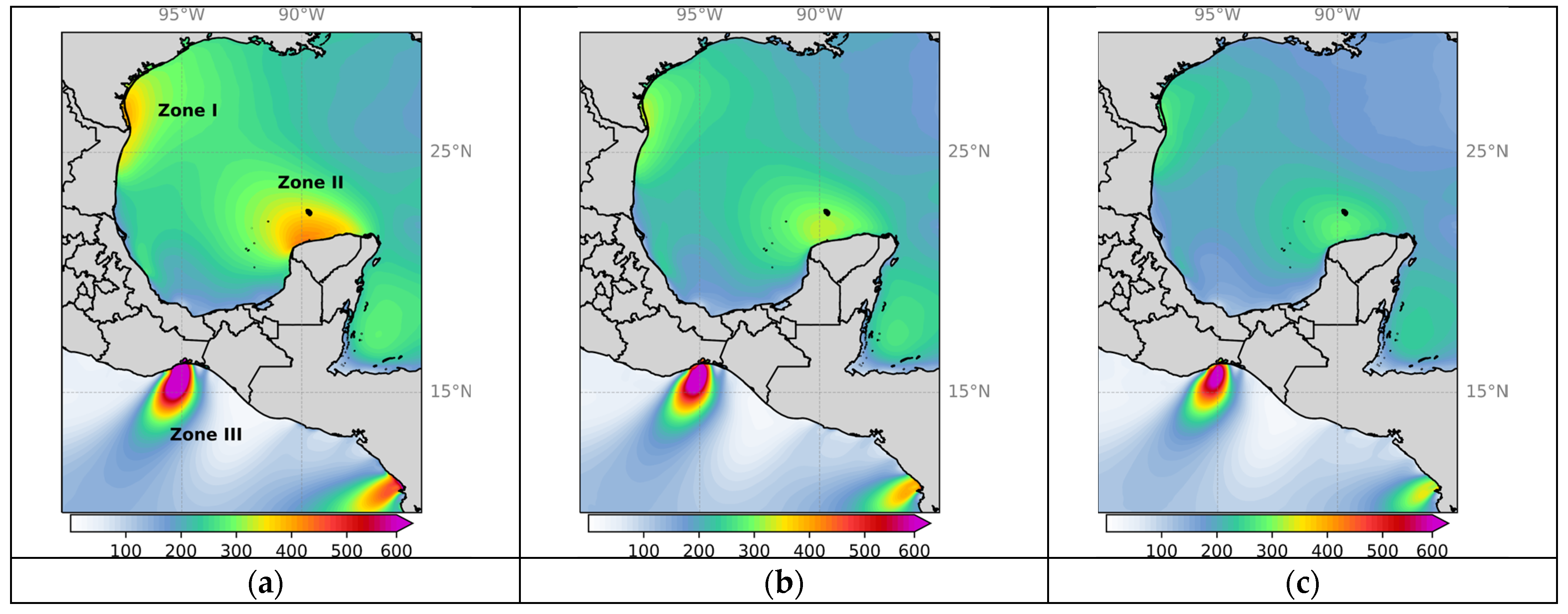
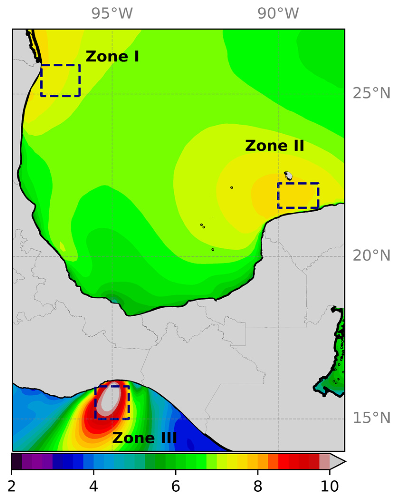
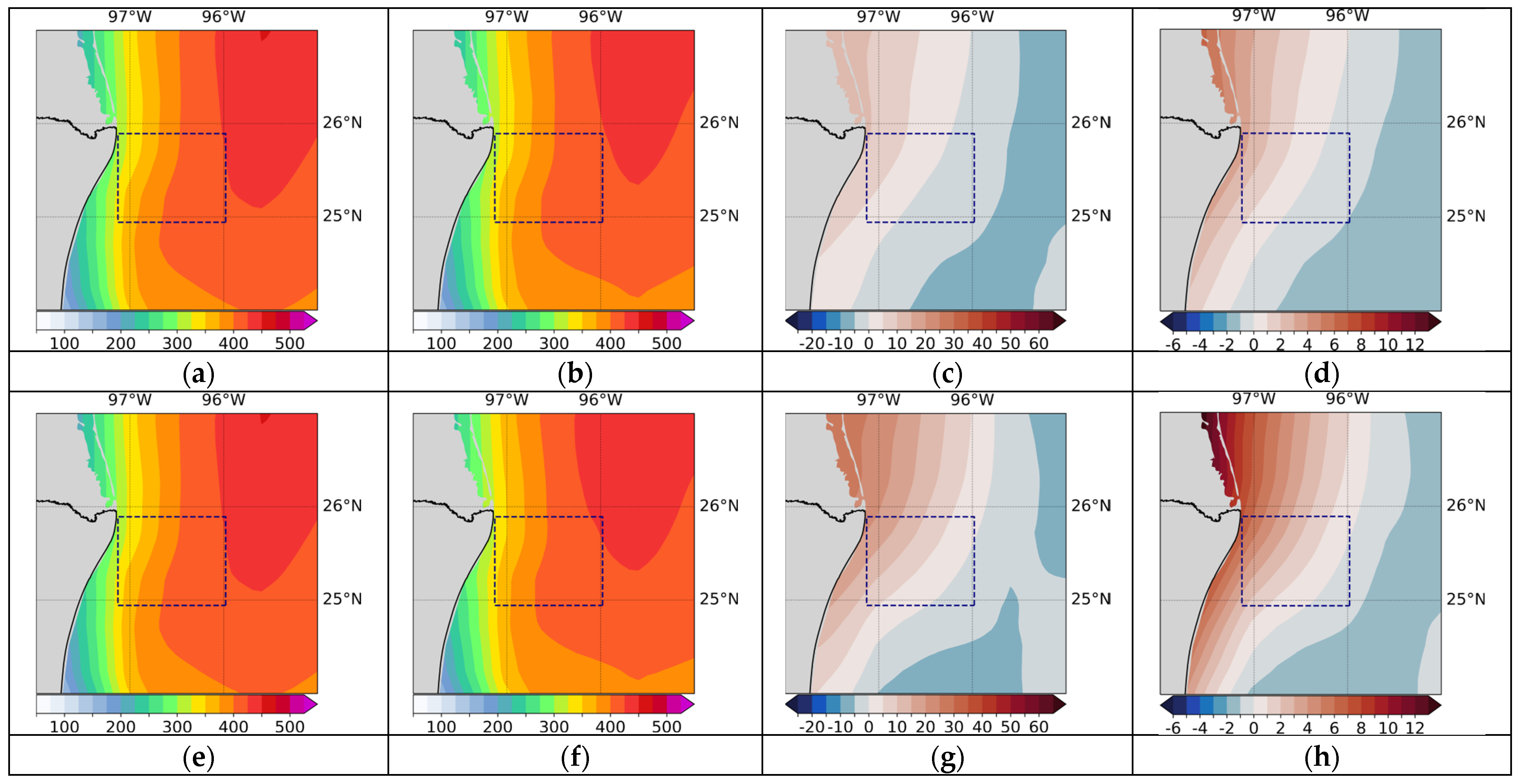
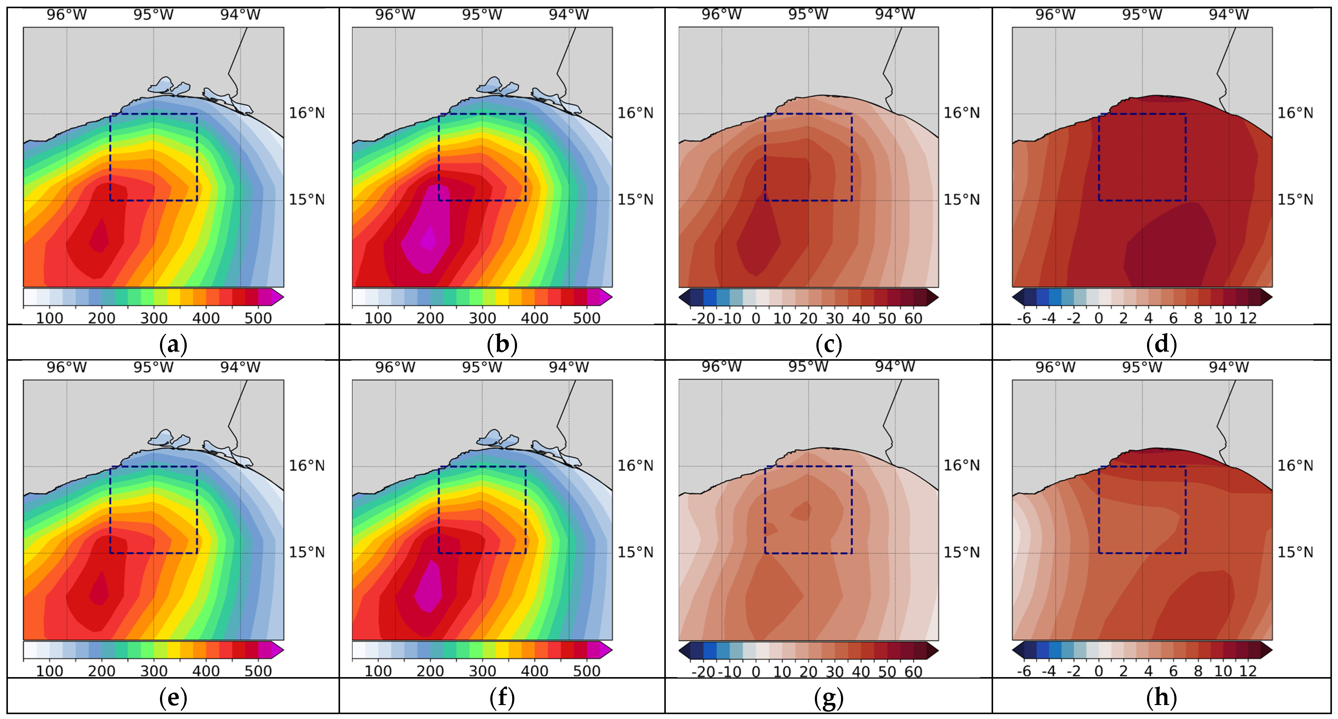
3.1. Identification of Areas with High Offshore Wind Potential in Mexico

To assess the feasibility of wind power at a site, wind power density is important. The formula for calculating wind power density is:

$$P=\frac{1}{2}\rho v^3$$

(6)

where $P$ is the power density (W/m²), $\rho$ is the air density (set at 1.225 kg/m³ for standard conditions, i.e., at sea level with a temperature of 15 °C and pressure of 1 atmosphere [61]), and $v$ is the wind speed (m/s). This approach is consistent with the typical initial phase of a wind resource assessment.

This study analyzes wind potential at 50, 100, and 200 m above ground level (AGL), all of which are within the levels considered in the Global Wind Atlas [62] and also fall within the range recommended by Lantz et al. [63], which suggests tower heights of 80 to 160 m AGL.

Figure 2 presents the annual wind power (W/m²) calculated from the WRF model data for the period 1979–2018, at three distinct altitudes: (a) 200, (b) 100, and (c) 50 m AGL. The maps distinctly highlight three key regions with substantial offshore wind power potential in Mexico: the north coast of Tamaulipas (Zone I), the northwest coast of Yucatan (Zone II), and the Gulf of Tehuantepec (Zone III). The wind power for Zones I and II is higher at higher altitudes, ranging from 300 to 400 W/m². For Zone III, the wind power remains constant for different altitudes, with intensities of up to 600 W/m².

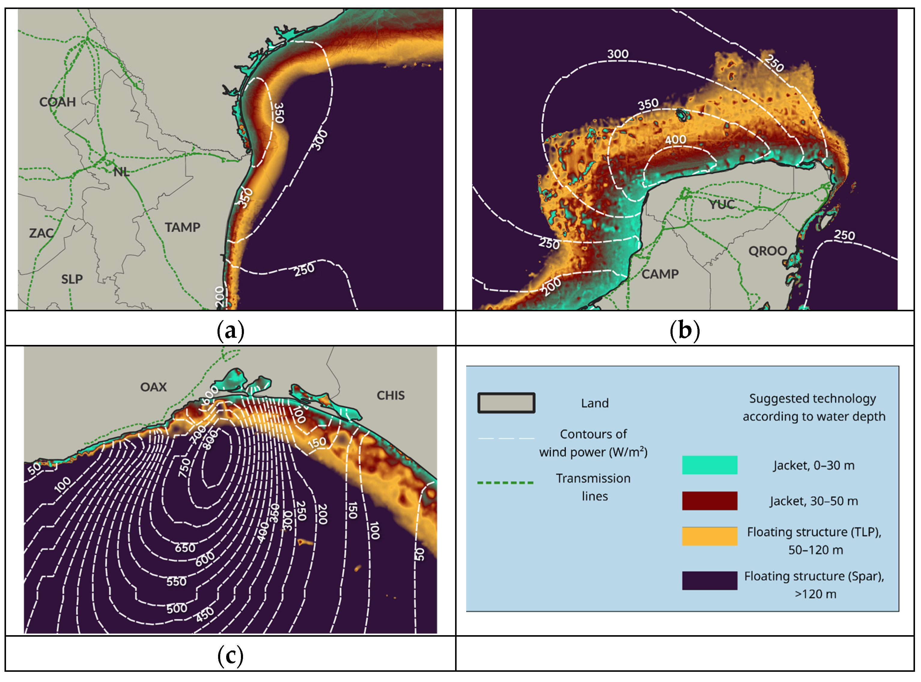
3.2. Bathymetry and Transmission Lines

Offshore grid connections play a crucial role in the viability of offshore wind energy, enabling the efficient transmission of power from offshore wind farms to onshore consumers. When it comes to deciding between AC (Alternating Current) and DC (Direct Current) for these connections, several factors come into play. Traditional advantages of AC, such as lower station costs, are important to consider. However, as distance and power capacity increase, transmission losses in AC systems become more significant.

On the other hand, DC connections offer lower cabling costs and lower losses over longer distances. The current trend in offshore wind projects, particularly in Europe’s North Sea, is leaning towards the adoption of high-voltage direct current (HVDC) transmission systems. These HVDC systems have proven to be operationally efficient and cost-effective, making them a popular choice for offshore wind connections. With the growth of offshore wind projects globally, the prospects for HVDC offshore wind connections remain promising, contributing to sustainable growth and the global shift towards cleaner energy sources [64].

In the context of offshore wind energy development, bathymetry plays an important role in determining the most suitable technology to harness wind resources. The water depth at a given offshore location directly impacts the type of foundation that can be used to support wind turbines. Table 4 outlines various foundation technologies tailored to distinct water depth ranges, as informed by references such as Nagababu et al. (2017) [65]. Figure 3 shows the offshore annual climatological wind potential at an elevation of 200 m for Zone I (a), Zone II (b), and Zone III (c), as well as the availability of nearby onshore power transmission lines and bathymetric characteristics.

Table 4. Foundation technologies for offshore wind turbines according to water depth range (Nagababu et al., 2017 [65]).

Water Depth Range (m)	Foundation Technology
0–30	Monopile/Gravity
30–50	Jacket/Tripod
50–120	Floating Structures (Tension Leg Platform and/or Semi-Submersible Type)
>120	Floating Structures (Spar Type)

Table 4. Foundation technologies for offshore wind turbines according to water depth range (Nagababu et al., 2017 [65]).

Water Depth Range (m)	Foundation Technology
0–30	Monopile/Gravity
30–50	Jacket/Tripod
50–120	Floating Structures (Tension Leg Platform and/or Semi-Submersible Type)
>120	Floating Structures (Spar Type)

Figure 3. Offshore wind potential (W/m²) (white segmented contours), onshore power transmission lines (green dashed lines), and suitable foundation technologies (color contours according to legend) for: (a) Zone I, (b) Zone II, and (c) Zone III.

Figure 3. Offshore wind potential (W/m²) (white segmented contours), onshore power transmission lines (green dashed lines), and suitable foundation technologies (color contours according to legend) for: (a) Zone I, (b) Zone II, and (c) Zone III.

One viable option for Mexico would be the utilization of HVDC transmission systems. This choice is primarily driven by the presence of transmission lines located within a distance of less than 100 km from the coastline (Figure 3). By adopting HVDC technology, Mexico can leverage its advantages, such as enhanced efficiency and reduced energy loss during long-distance transmission. Furthermore, by proactively considering the future development of offshore wind farms in Mexico, incorporating HVDC transmission infrastructure from the outset would facilitate a more seamless and cost-effective integration of the energy generated by these projects into the national grid. This strategic approach aligns with Mexico’s commitment to sustainable growth and the global transition towards cleaner energy sources.

On the other hand, in terms of bathymetry, one possible approach would involve considering the foundation technologies for offshore wind turbines outlined in Table 4, which are based on water depth ranges [65]. For Zones I and II, where the water depths allow for fixed foundations, Monopile/Gravity and Jacket/Tripod structures could be considered as suitable options. However, in Zone III of the Gulf of Tehuantepec, where the bathymetric features are more variable compared to the other two zones, alternative options such as Floating Structures could be explored (Figure 3). This suggestion takes into account the underwater conditions in Zone III and aims to optimize the effectiveness of offshore wind energy infrastructure in this specific region.

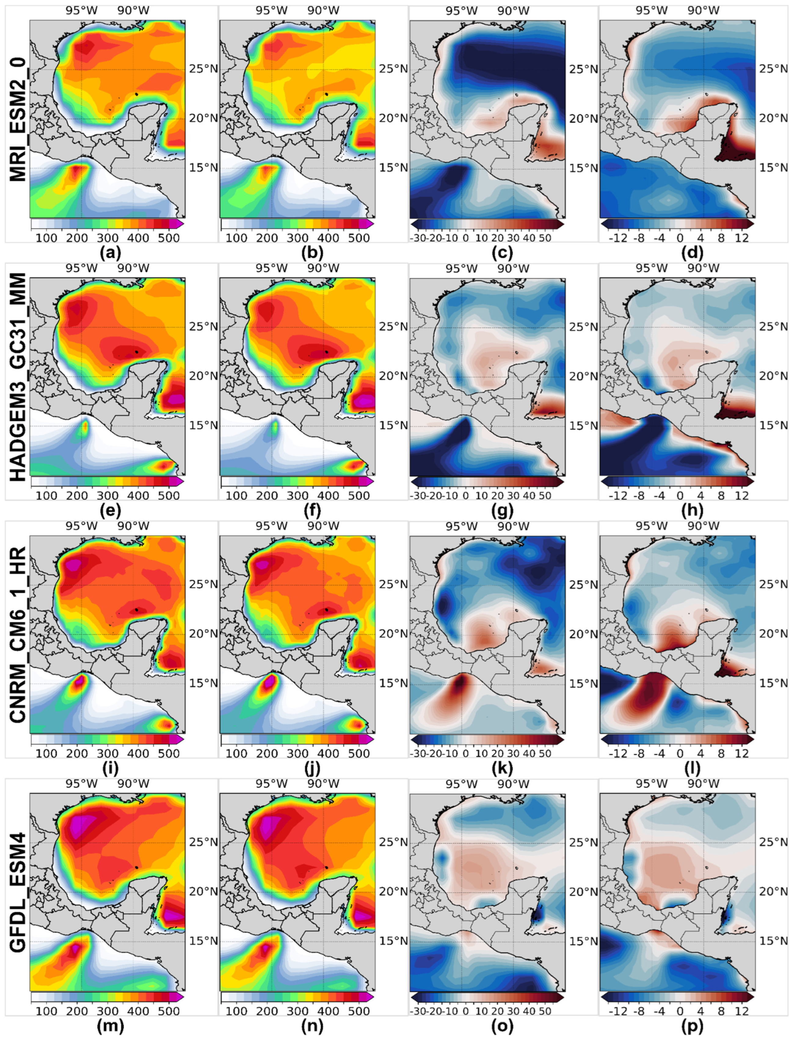
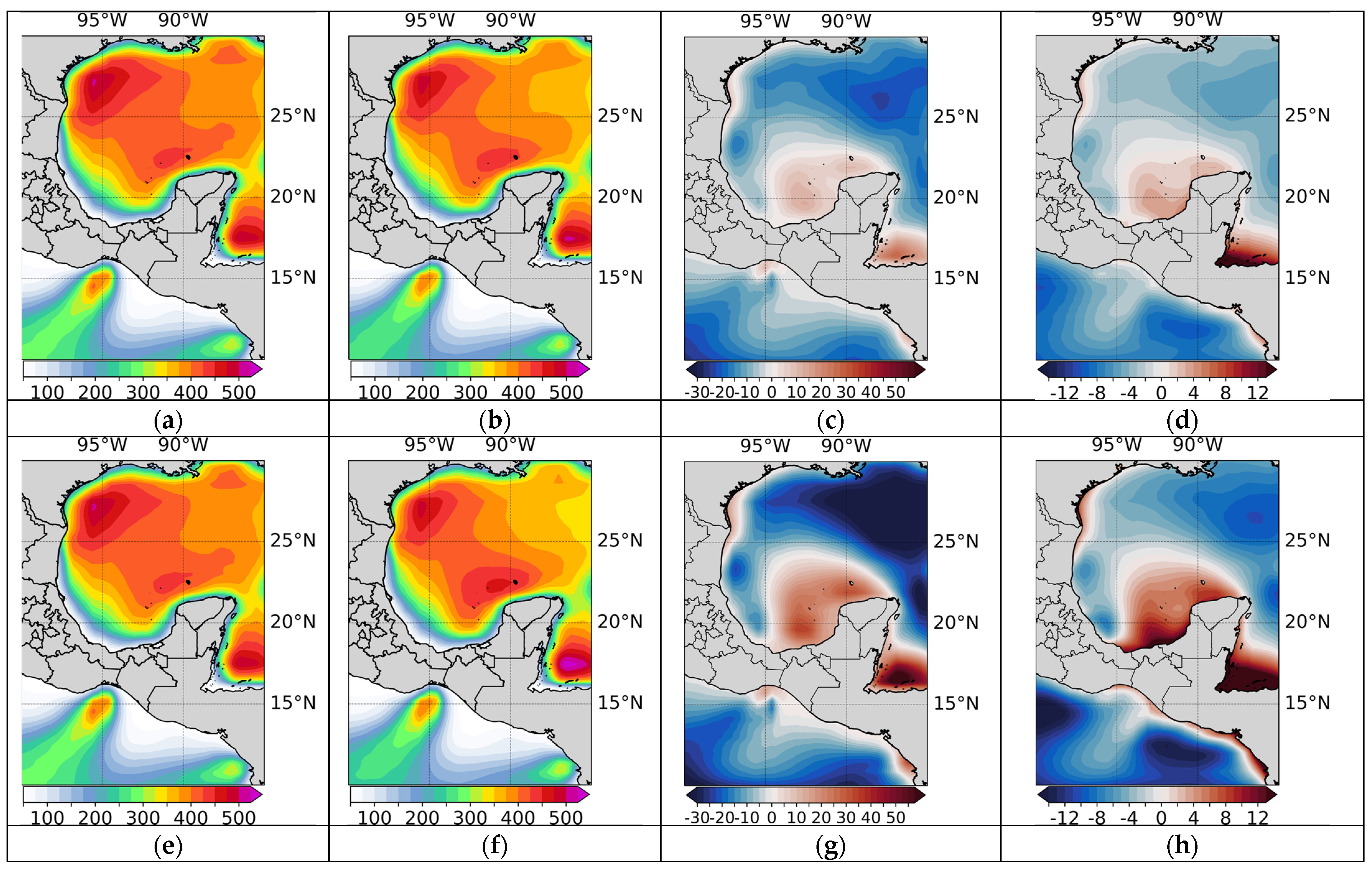
3.3. Comparison between CMIP6 Models and WRF

A comparative analysis between the WRF simulations and data from the CMIP6 models for the average wind speeds at 50 m AGL in the three marine zones with high wind potential is presented below. For this analysis, the CMIP6 time series that were previously adjusted by bias correction and variability adjustment were used. To perform this, three regions were delimited in which the maximum values of wind speed occur in each zone. Delimitation of these regions is achieved by identifying polygons that enclose each area of interest (

Table 5. Geographic coordinates of the vertices that delimit each region within the zones of interest.

Zone Name	Coordinates of the Vertices
Tamaulipas	(24.94, −97.12), (25.89, −97.12), (24.94, −95.97), (25.89, −95.97)
Yucatán	(21.5, −90), (22.25, −90), (21.5, −88.8), (22.25, −88.8)
Tehuantepec	(15, −94.5), (16, −94.5), (15, −95.5), (16, −95.5)

and Figure 4). In order to ensure a greater reliability of the results, our search for models within each target region considered the various configurations inherent to CMIP6 models, which dictate their complexity and resolution. By selecting the models that exhibit the greatest similarity, we aim to improve the robustness of our analysis.

For this analysis, we focused on the period 1985–2014, which was chosen because it encompasses data from all the models included in our study (Table 2), allowing for a comprehensive analysis of wind patterns over nearly three decades. The criteria used in the model selection process included a maximum limit of 20% for the MAPE. However, it is worth noting that the metrics used to estimate similarity errors are consistent with the MAPE results. In other words, models that perform well in terms of MAPE also show good results in metrics such as Pearson correlation, MAE, and RMSD. Likewise, the Minkowski Distance similarity metric also shows consistency, which can be seen in the region-specific tables presenting these scores, arranged based on the best MAPE for each CMIP6 model. By considering not only the MAPE but also the consistency of other similarity metrics, we ensure that the selected models provide reliable and robust results for the analysis of wind patterns in each target region.

The metrics were computed considering the average of all nodes within each region delimited in the three zones of interest in order to determine the similarity between the WRF model and each of the 47 CMIP6 models. The analysis of each region was performed individually, and different methods of comparison and evaluation were used. The outcome of these comparative analyses for each area of interest is detailed below.

The north coast of Tamaulipas (Zone I): 

Table 6. Values of the statistical metrics for the CMIP6 models that presented the best performance on the north coast of Tamaulipas (Zone I).

Model	MAPE	Pearson Correlation	RMSD (m/s)	MAE (m/s)	Minkowski Distance (m/s)
EC_EARTH3_VEG_LR	7.619	0.855	0.700	0.553	2.452
MRI_ESM2_0	7.665	0.829	0.691	0.544	2.529
EC_EARTH3_CC	7.821	0.826	0.700	0.563	2.291
HADGEM3_GC31_MM	7.933	0.852	0.702	0.572	2.423
CNRM_CM6_1_HR	7.967	0.824	0.701	0.568	2.479
CNRM_CM6_1	8.025	0.833	0.717	0.573	2.459

presents the values of the different metrics obtained for the CMIP6 models that showed the best performance in Zone I, considering the WRF data as the baseline. Taking all of the metrics into account as a whole, it can be considered that the EC_EARTH3_VEG_LR model showed the best performance for simulating the wind conditions in the region. However, similar values were obtained for the other five models in Table 6.

Below are comparisons of the time series of monthly averages (Figure 5) and annual cycles (Figure 6) of wind speed at 50 m AGL between the best performing models in Zone I (see Table 6) and the WRF data, considering the historical period of 1985–2014. It is observed that, in general, the models adequately reproduce the seasonal variation in the wind, although not necessarily the interannual variability, and that they overestimate the wind magnitude in this region (Figure 5). The average annual cycle in Zone I, based on the WRF data, shows stronger winds from November to April, with values between approximately 7.8 m/s and 8.3 m/s, and weaker winds in August and September, with values of approximately 5.5 m/s and 5.75 m/s, respectively (Figure 6). Figure 6 clearly shows the overestimation of the wind speed by the models, which is more evident during the winter months when winds are more intense.

The northwest coast of Yucatan (Zone II): In

Table 7. Values of the statistical metrics for the CMIP6 models that presented the best performance off the northwest coast of Yucatan (Zone II).

Model	MAPE	Pearson Correlation	RMSD (m/s)	MAE (m/s)	Minkowski Distance (m/s)
KACE_1_0_G	5.018	0.594	0.481	0.378	1.825
HADGEM3_GC31_MM	5.024	0.639	0.473	0.375	1.717
CNRM_CM6_1_HR	5.133	0.587	0.489	0.388	1.885
GFDL_ESM4	5.352	0.622	0.492	0.403	1.698

, the outcomes for the CMIP6 models showcasing the best performance off the northwest coast of Yucatan (Zone II) are provided. Examining the various statistical metrics, it is observed that the HADGEM3_GC31_MM model has the lowest RMSD, MAE, and Minkowski Distance and the highest Pearson correlation compared to the other three models in Table 7. In this region, the models present lower MAPE, RMSD, MAE, and Minkowski Distance values than those obtained for Zone I; however, the correlation coefficients turned out to be lower. This shows the importance of calculating various statistical metrics to carry out an evaluation of the models.

Figure 7 and Figure 8 show the comparative plots of the time series of the monthly averages and annual cycles, respectively, of the wind speed at 50 m AGL obtained from the WRF data and the CMIP6 models that showed better performance in Zone II. From Figure 7, it is observed that the time series obtained from the WRF data shows greater variability in Zone II compared to Zone I, which has an impact on the values obtained for the Pearson correlation coefficient. However, the four models adequately represent the average annual cycle in the region (with a discrepancy from the CNRM_CM6_1_HR model in June) (Figure 8). The annual cycle on the northern coast of Yucatan is somewhat different from that in Zone I (north coast of Tamaulipas), presenting average maximum winds from March to June, with values between approximately 7.85 m/s and 8.20 m/s, although the weakest winds also occur in August–September but with magnitudes higher than those in Zone I.

The Gulf of Tehuantepec (Zone III): In

Table 8. Values of the statistical metrics for the CMIP6 models that presented the best performance in the Gulf of Tehuantepec (Zone III).

Model	MAPE	Pearson Correlation	RMSD (m/s)	MAE (m/s)	Minkowski Distance (m/s)
FGOALS_F3_L	11.996	0.802	1.379	1.070	5.126
BCC_CSM2_MR	13.404	0.817	1.430	1.162	5.043
CNRM_CM6_1_HR	15.248	0.789	1.656	1.334	5.814
MRI_ESM2_0	17.555	0.759	1.914	1.594	6.089
GFDL_ESM4	17.761	0.827	1.878	1.549	6.592

, the results for the CMIP6 models showing the best performance in the Gulf of Tehuantepec (Zone III) are presented. In general, the metrics obtained for the FGOALS_F3_L model highlight its better performance in simulating the monthly winds in Zone III. The time series of the monthly averages of wind speed at 50 m above the surface (Figure 9) clearly shows that the models underestimate the magnitude of the winds during the summer. This underestimation is also noted in the comparison of the mean annual cycles (Figure 10), where it can be seen that none of the models considered to have the best performance reproduce the relative maximum of the wind magnitude during July and August, which is a characteristic feature of this region [66] and is well represented in the WRF data.

3.4. CMIP6 Ensembles: Projecting Future Wind Power

After the evaluation of the CMIP6 models, ensembles were generated to analyze future projections regarding the offshore wind potential in the three regions of interest. One option was to consider the ensemble average by equally averaging the model outputs. However, this approach may lead to a lower performance by treating all models equally. In contrast, the weighted average ensemble assigns specific weights to each model [67], prioritizing those that showed a better performance. Nonetheless, for a comprehensive analysis, both the ensemble average and the weighted average ensemble were calculated.

3.4.1. Ensemble Average

The ensemble average was applied to the set of CMIP6 models that performed best in their evaluation and appeared in at least two of the three zones of interest.

Table 9. List of the best performing CMIP6 models for each region, highlighting those that appeared in at least two of them.

Model	Zona I	Zona II	Zona III
BCC_CSM2_MR			✓
EC_EARTH3_VEG_LR	✓
MRI_ESM2_0	✓		✓
EC_EARTH3_CC	✓
HADGEM3_GC31_MM	✓	✓
CNRM_CM6_1_HR	✓	✓	✓
CNRM_CM6_1	✓
FGOALS_F3_L			✓
GFDL_ESM4		✓	✓
KACE_1_0_G		✓

shows which CMIP6 models were chosen to generate the ensemble average: MRI_ESM2_0, HADGEM3_GC31_MM, CNRM_CM6_1_HR, and GFDL_ESM4.

Before calculating the ensemble average, an analysis was carried out that consisted of comparing the wind potential’s historical climatology (1985–2014) with the short-term (2040–2069) and long-term (2070–2099) projections considering the selected CMIP6 models. The climatologies were determined by averaging the monthly data. Absolute differences and percentage differences between the projections and the historical climatology were calculated to assess trends using the following equations:

$$Absolutedifference=\left|CMIP{6}_{proj}-CMIP{6}_{hist}\right|$$

(7)

$$Percentagedifference=\frac{\left|CMIP{6}_{proj}-CMIP{6}_{hist}\right|}{CMIP{6}_{hist}}\times 100$$

(8)

Absolute difference measures the numerical change in wind potential between the projected and historical periods, providing a direct indication of the magnitude of the change in units of W/m². Percentage difference expresses this change as a percentage of the historical wind potential, and therefore, is a dimensionless quantity. Together, these quantities allow the expected variations in wind potential over time to be quantified and compared, providing valuable information on the scale and relative significance of such changes.

Figure 11 presents the results of the comparative analysis between the historical (Figure 11a,e,i,m) and short-term (2040–2069) projections (Figure 11b,f,j,n) for each selected CMIP6 model. It becomes apparent that the historical and climate projection maps exhibit variations between the different models.

Particularly in Zone III, the HADGEM3_GC31_MM model shows a significant underestimation of wind potential (Figure 11g), accompanied by a negative percentage difference (Figure 11h). The MRI_ESM2_0 model also exhibits a negative percentage difference for Zone III (Figure 11d), in contrast to those of the CNRM_CM6_1_HR and GFDL_ESM4 models, which suggest positive percentage differences (Figure 11l,p). This implies that Zone III might benefit from a more detailed ensemble approach, such as the weighted average ensemble. In general, for Zones I and II, more consistent results are obtained between the models, indicating positive percentage differences (Figure 11d,h,l,p) that suggest an increase in wind potential in these zones for the short-term period.

Figure 12 presents a comparative analysis similar to the previous one but for the long-term projection (2070–2099), showing similar results to those of the short-term period for each model. It is important to highlight that the existing patterns are accentuated in the long-term period, which suggests a greater increase in wind potential for Zones I and II.

Next, the ensembles average for wind power from the selected models (see Table 9), both for the short-term and long-term projections compared to the historical mean, are shown in Figure 13. It is evident in Zones I and II that there is a positive percentage difference in the short term, which is significantly accentuated in the long-term projection. In Zone III, a positive percentage difference is observed close to the coast and negative values offshore.

3.4.2. Weighted Average Ensemble

The method used to obtain the weighted average ensemble from the CMIP6 models is based on calculating the contributions of each model according to its similarity with the reference WRF model in each of the three zones, based on the lowest MAPE values obtained previously. The procedure is described in

Table 10. Procedure for calculating the weighted average ensemble.

Description	Equation
Equation for calculating the weights based on the inverse of the squared MAPE.	$w_i=\frac{1}{{MAP{E}_i}^2}$
Equation for normalizing the weights.	$w_{i}normalized=\frac{w_i}{{\sum }_{i=1}^n{w}_i}=w_{i}n$
Equation for calculating the weighted ensemble using the normalized weights.	$Ensemble={\displaystyle \sum _{i=1}^n}{w}_{i}n\cdot x_i$

.

Detailed below are the results of the weighted average ensembles for the set of CMIP6 models that showed the best performance in each zone of interest, emphasizing the delimited areas within each zone (see Figure 4). It is important to remember that the set of models differs for each zone (see Section 3.3). Weighted means are calculated for the historical period (1985–2014) and the short-term (2040–2069) and long-term (2070–2099) projections for each zone. After estimating these values, a comparative analysis is carried out using the absolute and percentage differences between the historical mean and both future projections.

The north coast of Tamaulipas (Zone I): Figure 14 presents the weighted ensemble results for Zone I. In this case, the models considered include EC_EARTH3_VEG_LR, MRI_ESM2_0, EC_EARTH3_CC, HADGEM3_GC31_MM, CNRM_CM6_1_HR, and CNRM_CM6_1 (see Table 6). The map of the absolute difference for the short-term projection reveals, in general, relatively low values (between −5 and 10) within the delimited area (Figure 14c), while the percentage differences are between −1% and 4% (Figure 14d). An increase in positivity is observed for the long-term projection, both in absolute and percentage differences (Figure 14g,h). In particular, coastal areas exhibit larger percentage deviations, of about 3–4% for the short-term projection and 6–7% for the long-term projection, which gradually decrease offshore where small negative values can be observed.

The northwest coast of Yucatan (Zone II): The models considered for the weighted ensemble average in Zone II include KACE_1_0_G, HADGEM3_GC31_MM, CNRM_CM6_1_HR, and GFDL_ESM4 (see Table 7). Similar to what was observed in Zone I, in Zone II positive absolute and percentage differences with respect to the historical average are evident for the short-term projection (Figure 15c,d), and become more pronounced for the long-term projection (Figure 15g,h). However, in this case, the largest deviations are not observed along the coast but in the center of the delimited region, with values that reach around 4–5% in the percentage difference for the short-term projection and around 8–9% for the long-term period. This suggests that this area may possess the most favorable conditions for the development of an offshore wind park in Zone II.

The Gulf of Tehuantepec (Zone III): The models considered for the weighted average ensemble in Zone III include: FGOALS_F3_L, BCC_CSM2_MR, CNRM_CM6_1_HR, MRI_ESM2_0, and GFDL_ESM4 (see Table 8). The map of the percentage difference for the short-term projection (Figure 16d) shows values between 9% and 10% within the delimited area, while in a small area very close to the coast, values greater than 10% are reached. Values greater than 10% also occur in Zone III in a wide region to the south (offshore) of the delimited area. For the long-term projection, the values of the percentage differences within the delimited area are between 6% and 8%, while near the coast the values exceed 9% (Figure 16h). In Zone III, the differences between the future projections and the historical average show the highest values towards the center of the area and decrease towards the eastern and western extremes.

4. Discussion

Next, we delve into a discussion of the main results of this study, making comparisons with previous studies.

(1)

Identification of high wind potential areas and recommendations for foundation technologies: Three areas with significant offshore wind potential in Mexico were identified through relatively high spatial resolution (~10 km) numerical simulations with the WRF model for the 40-year period of 1979–2018: the north coast of Tamaulipas (Zone I), the northwest coast of Yucatan (Zone II), and the Gulf of Tehuantepec (Zone III). These areas have been studied in other works under different approaches. Among them, Canul-Reyes et al. [9] assessed offshore wind potential in the Gulf of Mexico based on data from the ERA5 and MERRA2 reanalyses (~30 and 50 km resolution, respectively), identifying promising areas for development based on geographical restrictions, wind speed analysis, and capacity factor seasonal variability. They identified the north coast of the Tamaulipas state and the northwest of the Yucatan peninsula as the areas with the greatest potential for offshore wind energy development in the Gulf of Mexico.

On the other hand, Bernal-Camacho et al. [11] identified the Gulf of Tehuantepec as a promising location in the Mexican Pacific for wind energy harvesting. This study carried out a technical evaluation to analyze the feasibility of installing a floating offshore wind turbine platform, according to the most probable and extreme maritime conditions in the region. The authors concluded that such technology could be suitable for installation in the Gulf of Tehuantepec. According to our analysis of the bathymetric characteristics of Zone III, the implementation of floating foundation technologies would be the most convenient, which alignes with the results of Bernal-Camacho et al. [11]. For the other two zones, located in the Gulf of Mexico, fixed-foundation technologies would be the most appropriate. Additionally, and based on the arrangement of transmission lines located less than 100 km from the coast in the three identified zones, the use of HVDC transmission systems is suggested due to their greater efficiency and lower energy loss, in addition to the fact that it would promote a more fluid and profitable integration of the energy generated by offshore wind farms on the national grid.

(2)

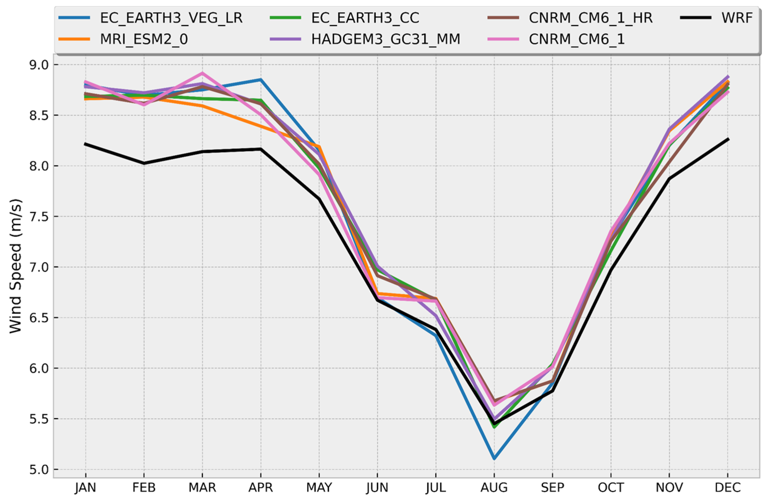
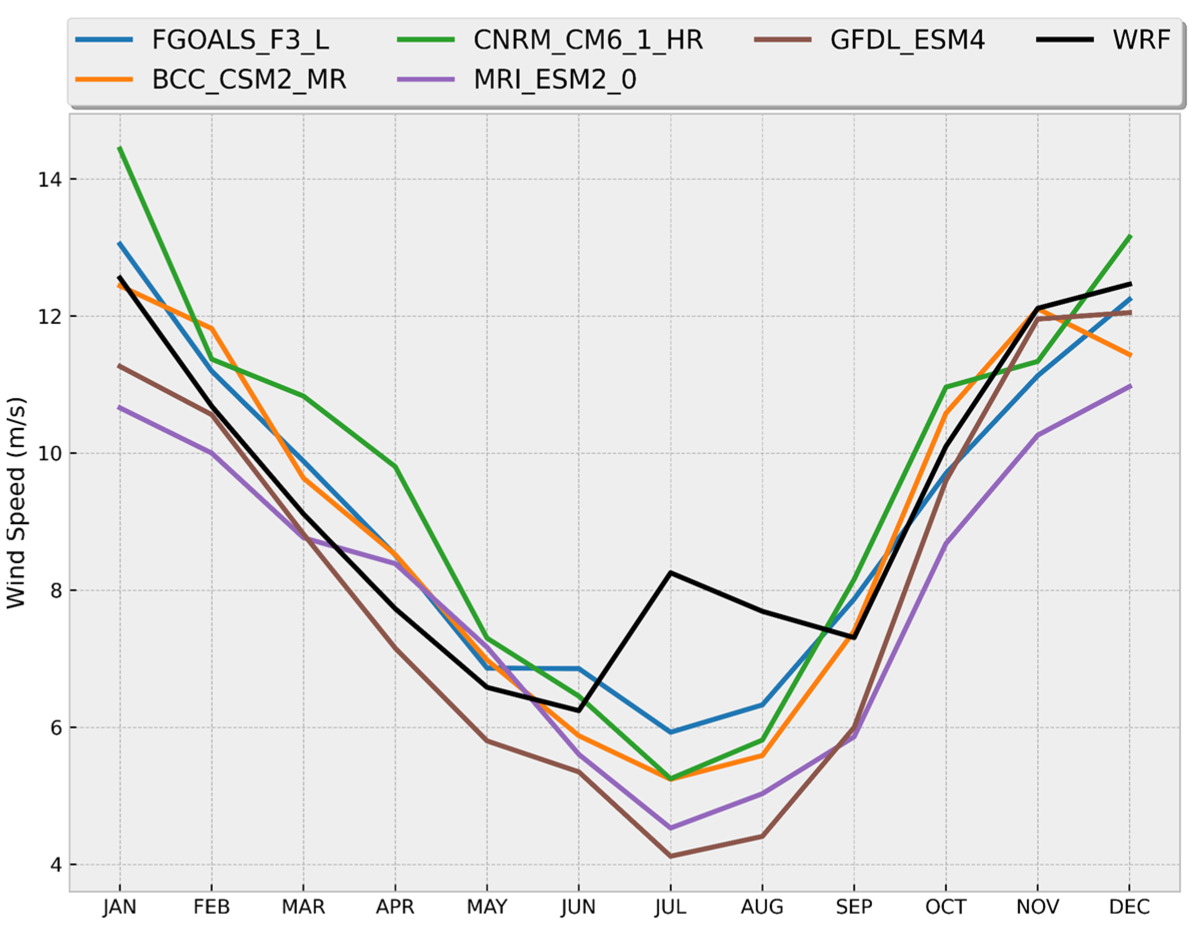
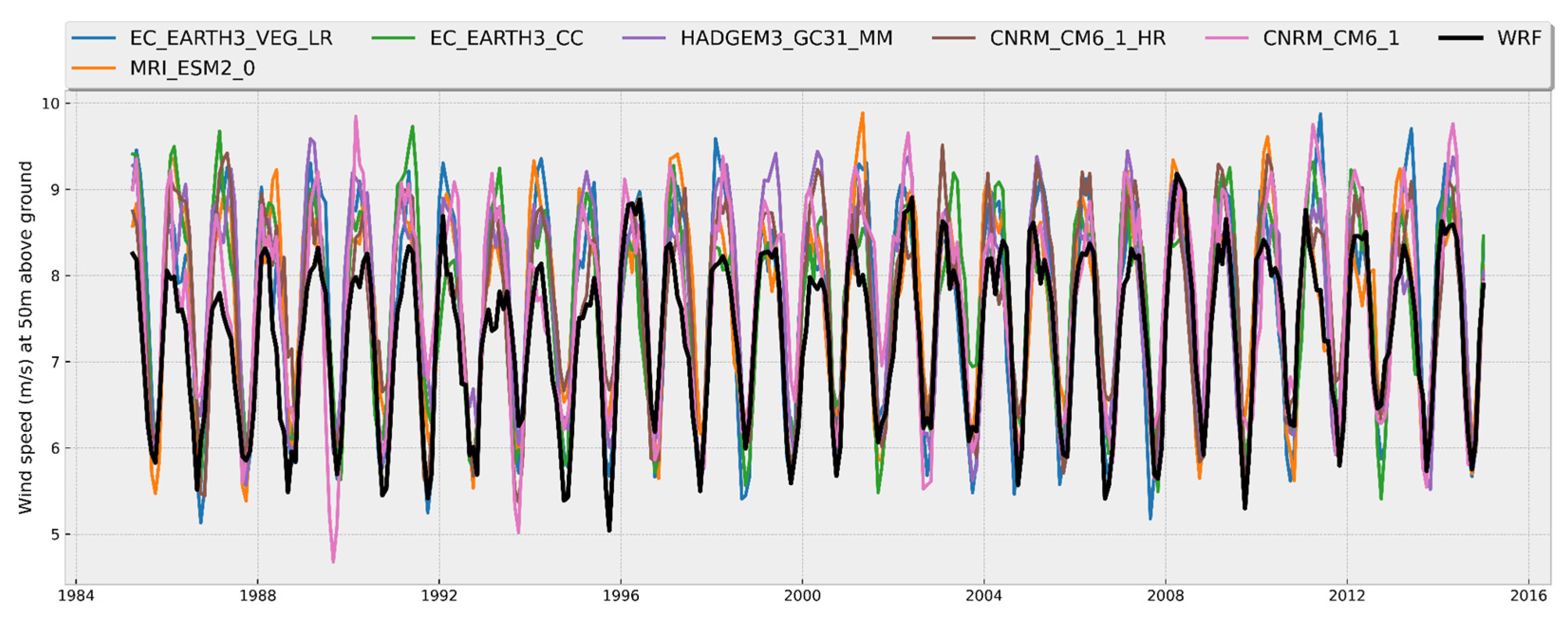
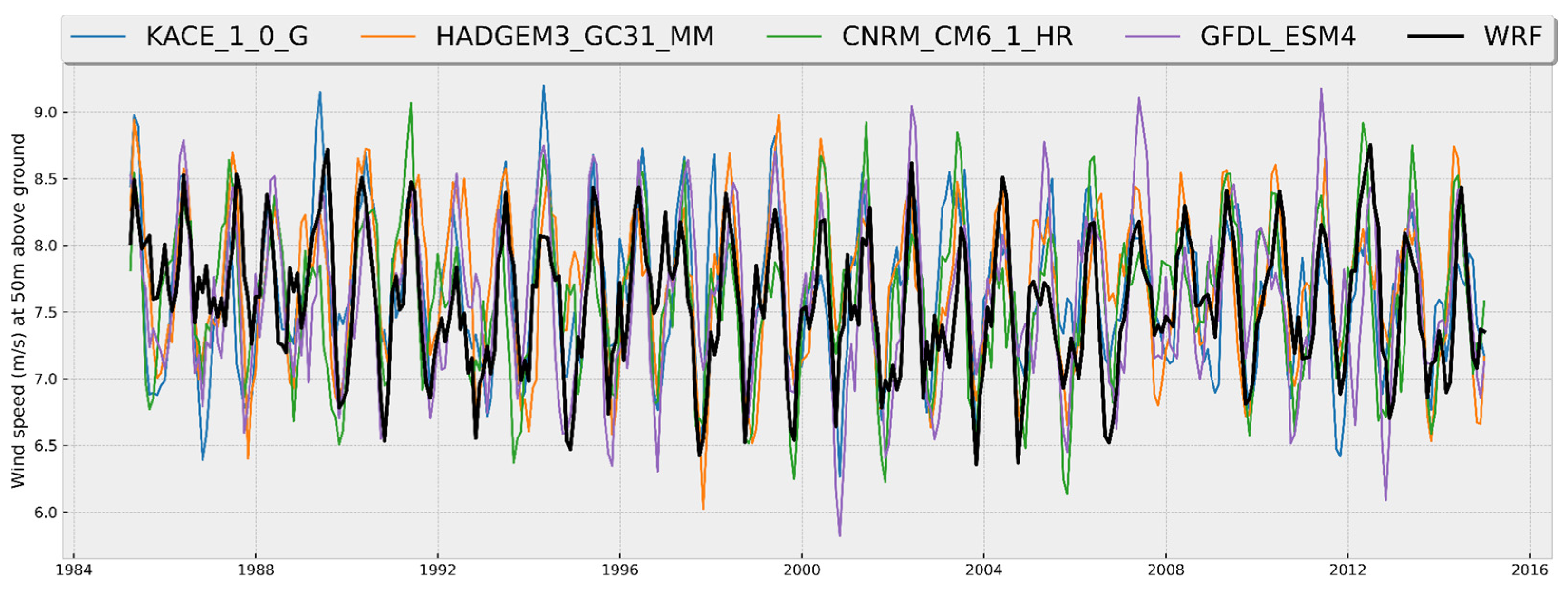
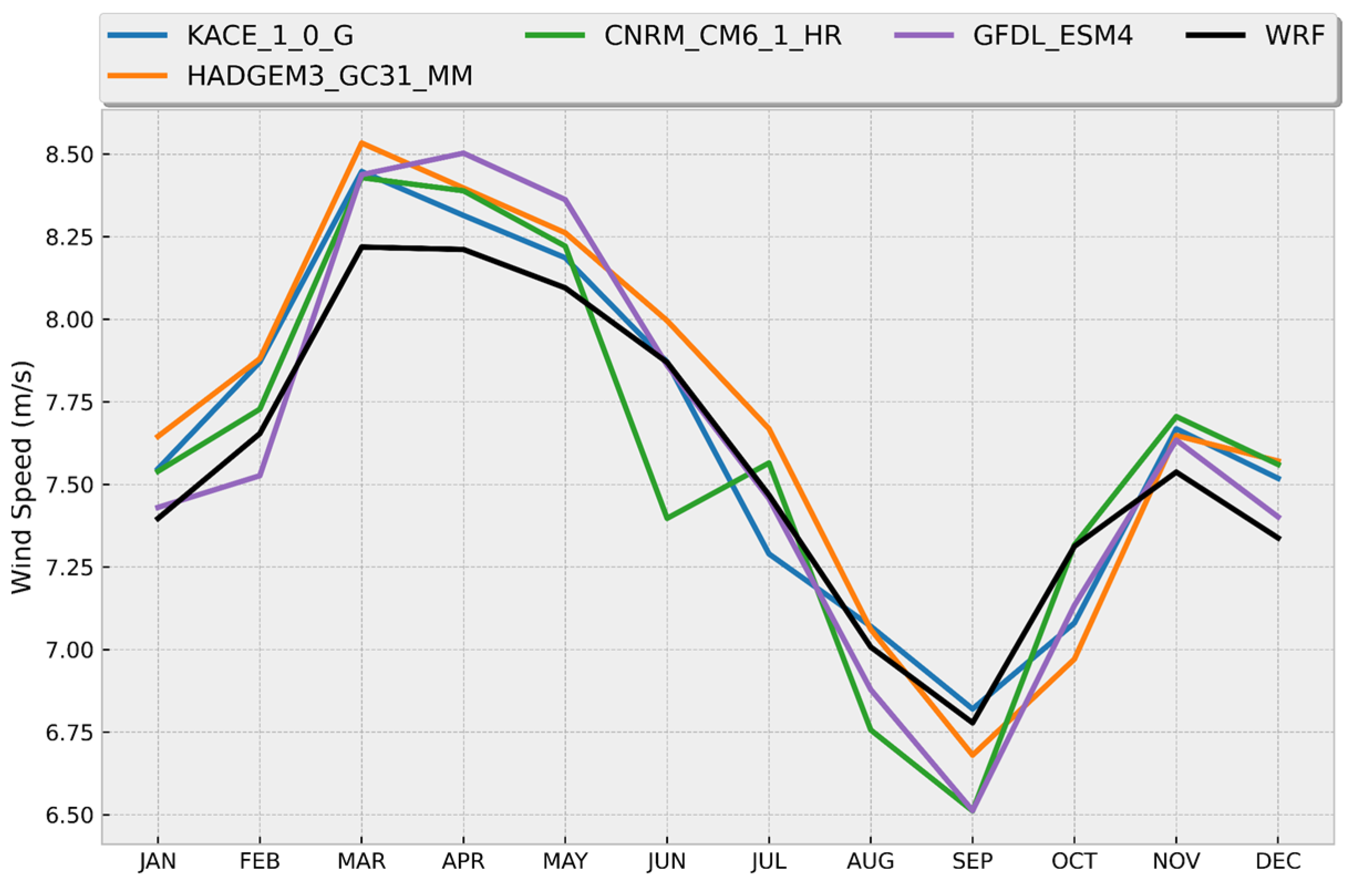
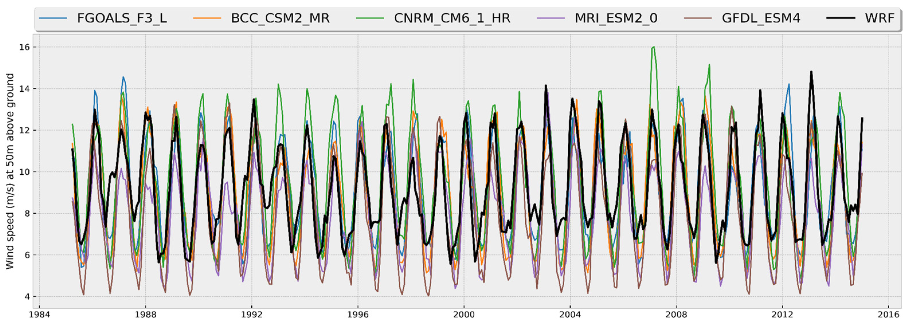
Model performance: A comparative analysis was carried out of the time series of monthly averages and annual cycles of wind magnitude at 50 m above the surface, obtained from the WRF data and the best performing CMIP6 models in the three zones of interest for the historical period 1985–2014. The results indicated that, in general, the CMIP6 models adequately reproduce seasonal variations and annual cycles, although not necessarily the interannual variability, with a certain over or underestimation of the values depending on the time of year and the particular zone. Each zone shows particular behaviors throughout the year in terms of the variable analyzed. For example, the annual cycle in Zone I (see Figure 6) shows a range of values approximately between 5.50 and 8.30 m/s, with stronger winds between December and April and weaker ones in August and September. In Zone II, winds with a greater interannual variation are observed compared to the other two zones (see Figure 7), which influenced the lower values of the correlation coefficient we obtained. Its annual cycle shows a smaller range of variation, with values between approximately 6.75 and 8.25 m/s; however, the most intense winds occur between March and May and not during the winter months (see Figure 8). This is a zone that is predominantly affected by the easterly trade winds which flow parallel to the coast throughout the year, while in Zone I the predominant winds change direction throughout the year and most of the time flow from sea to land coming from the southeast [68]. The above indicates that the dynamic processes that determine the high wind potential in both areas are different. The results obtained in the present study are in accordance with the analyses of the monthly averages of the capacity factor in these two areas of the Gulf of Mexico carried out by Canul-Reyes et al. [9]. In general, they obtained the maximum values between March and April and the minimum values from July to September in those regions, which coincides with our analysis of the annual cycle of wind magnitude.

Zone III, for its part, shows a bimodal behavior in the annual cycle of wind magnitude, with higher values during winter (~10.5–12.3 m/s) that decrease towards summer (minimum values of ~6.2 m/s) but with a slight increase in the months of July–August (~8.2 m/s and 7.7 m/s, respectively) (see Figure 10). This characteristic has been reported in previous works and it is associated with an increase in the pressure gradient between the Gulf of Mexico and the Gulf of Tehuantepec that causes an intensification of the northerly winds that cross through the mountainous gap that exists in the region [66]. Apparently, this topographic feature is not well represented in the CMIP6 models, given its horizontal resolution, resulting in an underestimation of the wind magnitude in Zone III during these months (see Figure 10).

(3)

Future projections of offshore wind energy potential: In this work, two types of CMIP6 model ensembles were tested in order to analyze the future projections of offshore wind potential considering a short-term (2040–2069) and a long-term (2070–2099) period under the SSP5-8.5 scenario: the ensemble average and the weighted average ensemble. The latter was obtained by calculating the contribution of each CMIP6 model according to its similarity with the climatological conditions of the wind magnitude computed from the WRF reference model for each of the three analyzed zones. To do this, the smallest MAPE values for each zone were considered (see Table 6, Table 7 and Table 8). The result is a weighted-average ensemble which assigns specific weights to each model, prioritizing those that showed better performance in each area, unlike the ensemble average that considers them all equally. In this sense, we consider that the weighted average ensemble yields more consistent, reliable, and robust results compared to the average ensemble.

Then, a comparative analysis was carried out using the absolute and percentage differences between the historical mean (1985–2014) and both future projections. In general, the results show certain regions in which both future projections estimate an increase in wind potential, with higher values for the long-term period (see Figure 14, Figure 15 and Figure 16). In terms of the percentage differences with respect to the historical climatology, the ensemble showed the highest values in Zone III for the long-term projection, reaching 10% very close to the coast and towards the central part of the region, where the most intense winds occur. In Zone II, values between 8% and 9% are reached in the center of the region, and in Zone I, the percentages reach values between 6% and 7% along coastal areas.

Some recent studies have investigated climate projections for offshore wind power in different regions using CMIP6 model outputs. The work of Thomas et al. [69] focused on the offshore wind energy potential in the Spanish territorial waters, finding increases of up to 15% particularly in the northwest of the Iberian Peninsula and the Canary Islands for the near future (2030–2059) under SSP5-8.5. On the other hand, Claro et al. [70] conducted a study on wind power density, finding statistically significant increases during the summer season off the northwest coast of Portugal and over the Serra da Estrela. The research also highlighted anomalies in wind direction during winter, with a westward shift over southern Portugal and the nearby ocean. These studies can be compared to ours in that they used a multi-model CMIP6 ensemble and the WRF atmospheric model. Although there may be differences in the methodologies used, these studies found similar trends in offshore wind energy potential for different geographic areas.

Finally, Martinez and Iglesias [71] conducted a study on offshore wind energy resources in the Mediterranean Sea using CMIP6 models and ERA5 data as the baseline, for different SSPs. Under the SSP5-8.5 scenario, an overall decrease of around 20% was projected particularly in the central and western Mediterranean, and up to 30% in other areas. These results are consistent with other large-scale studies using CMIP5 projections, but with more significant changes. However, discrepancies were observed when comparing wind projections with those from downscaling initiatives such as CORDEX. While studies employing GCMs provide a preliminary understanding of general trends in the Mediterranean Sea, they may not fully capture regional phenomena associated with smaller-scale dynamics. This confirms the importance of incorporating RCMs into climate projections, as we did in our study.

Overall, these findings would indicate that it could be viable and profitable to direct efforts to the construction of offshore wind farms in the three identified marine areas, taking into consideration the bathymetric characteristics and environmental conditions of each one, but without forgetting the fact that there is always uncertainty associated with future climate projections.

5. Conclusions

This study provides a comprehensive assessment of Mexico’s offshore wind energy potential using numerical climate modeling. Numerical simulations with the WRF model for a 40-year historical period allowed us to identify three offshore zones with different degrees of wind energy potential: the northern coast of Tamaulipas, the northwest coast of Yucatan, and the Gulf of Tehuantepec. Previous research highlights the importance of employing regional models to accurately capture climatic processes. Regional models, such as the WRF model, have been shown to effectively represent fine-scale features, topographical influences, and coastal effects [72,73], which are crucial factors for evaluating offshore wind energy potential.

The historical simulations generated with the WRF model served as a basis to identify the CMIP6 models that more accurately represented the climatological behavior of the wind magnitude in the areas of interest mentioned above. From these, ensembles were constructed using two methods: the simple average and the weighted average. The results show that the future projections of wind potential based on ensemble-weighted averages of the selected CMIP6 models for each zone, provide more reliable projections compared to the average ensemble. Weighted averaging optimizes accuracy and assesses climate change impacts on wind energy resources by prioritizing best CMIP6 models according to regional characteristics, such as coastal and marine contrasts.

In a comparable study, using the same emissions pathway (SSP5-8.5), substantial mid-term (2051–2060) and long-term (2091–2100) increases in wind resources were observed across various regions of North America [13]. Although the focus of such research is primarily on onshore wind resources, maps illustrating percentage differences in wind potential also include offshore regions. The results indicate a potential mid-term increase of approximately 10% in wind potential in the maritime zone off the north coast of Tamaulipas and in the Gulf of Tehuantepec, while the maritime zone off the northwest coast of Yucatan exhibits percentage differences close to zero, suggesting no significant changes in wind potential in that particular area. In the long-term, an increase in wind potential is observed only in the maritime zone off the north coast of Tamaulipas, while other areas do not show significant changes. In our study, we obtained positive percentage differences in wind power with respect to the historical average (1985–2014) in the three identified regions for the long-term projections (2070–2099). The values are around 6–7% along coastal areas off the north coast of Tamaulipas (Zone I), around 8–9% off the northwest coast of Yucatan (Zone II), and up to 10% very near the coast and at the center of the Gulf of Tehuantepec (Zone III).

Different regional approaches and model selection procedures lead to discrepancies in the results of different studies. The selected methodology must be appropriate for the specific objectives of each individual study, as different regions and timescales may justify tailored modeling approaches to resolve unique features at relevant spatial and temporal scales.

In particular, no previous research has focused specifically on analyzing the possible climate impacts on the wind potential of the marine areas of Mexico based on the CMIP6 models. Therefore, this regional analysis offers preliminary assessments of the capacity for offshore wind energy in Mexico in the context of climate change, which can help guide sustainable development opportunities in those areas. Improvements using higher resolution models would strengthen our understanding and future planning decisions. In conclusion, Mexico has important offshore wind resources that seem to be promising for use in the future. Doing so sustainably could bolster energy security while supporting national economic and climate mitigation goals.

References

1. Department of Energy. How Wind Can Help Us Breathe Easier. Energy.gov. Available online: https://www.energy.gov/eere/wind/articles/how-wind-can-help-us-breathe-easier (accessed on 7 September 2023).
2. Marvel, K.; Kravitz, B.; Caldeira, K. Geophysical limits to global wind power. Nat. Clim. Chang. 2013, 3, 118–121. [Google Scholar] [CrossRef]
3. Bailey, H.; Brookes, K.L.; Thompson, P.M. Assessing environmental impacts of offshore wind farms: Lessons learned and recommendations for the future. Aquat. Biosyst. 2014, 10, 8. [Google Scholar] [CrossRef] [PubMed]
4. Leung, D.Y.; Yang, Y. Wind energy development and its environmental impact: A review. Renew. Sustain. Energy Rev. 2012, 16, 1031–1039. [Google Scholar] [CrossRef]
5. Ellis, G.; Ferraro, G. The Social Acceptance of Wind Energy; Technical Report. JRC Science for Policy Report; European Commission: Brussels, Belgium, 2016. [CrossRef]
6. Wind Europe. Wind Energy in Europe: 2022 Statistics and the Outlook for 2023–2027. Available online: https://windeurope.org/intelligence-platform/product/wind-energy-in-europe-2022-statistics-and-the-outlook-for-2023-2027/#downloads (accessed on 7 September 2023).
7. Huacuz, J.M. The road to green power in Mexico—Reflections on the prospects for the large-scale and sustainable implementation of renewable energy. Energy Policy 2005, 33, 2087–2099. [Google Scholar] [CrossRef]
8. Bracho, R.; Alvarez, J.; Aznar, A.; Brancucci, C.; Brinkman, G.; Cooperman, A.; Flores-Espino, F.; Frazier, W.; Gearhart, C.; Guerra Fernandez, O.J.; et al. Mexico Clean Energy Report; (No. NREL/TP-7A40-82580), National Renewable Energy Lab. (NREL): Golden, CO, USA, 2022. [Google Scholar]
9. Canul-Reyes, D.A.; Rodríguez-Hernández, O.; Jarquin-Laguna, A. Potential zones for offshore wind power development in the Gulf of Mexico using reanalyses data and capacity factor seasonal analysis. Energy Sustain. Dev. 2022, 68, 211–219. [Google Scholar] [CrossRef]
10. Arenas-López, J.P.; Badaoui, M. Analysis of the offshore wind resource and its economic assessment in two zones of Mexico. Sustain. Energy Technol. Assess. 2022, 52, 101997. [Google Scholar] [CrossRef]
11. Bernal-Camacho, D.F.; Fontes, J.V.; Mendoza, E. A Technical Assessment of Offshore Wind Energy in Mexico: A Case Study in Tehuantepec Gulf. Energies 2022, 15, 4367. [Google Scholar] [CrossRef]
12. Martinez, A.; Iglesias, G. Wind resource evolution in Europe under different scenarios of climate change characterised by the novel Shared Socioeconomic Pathways. Energy Convers. Manag. 2021, 234, 113961. [Google Scholar] [CrossRef]
13. Martinez, A.; Iglesias, G. Climate change impacts on wind energy resources in North America based on the CMIP6 projections. Sci. Total Environ. 2022, 806, 150580. [Google Scholar] [CrossRef] [PubMed]
14. Shen, C.; Zha, J.; Li, Z.; Azorin-Molina, C.; Deng, K.; Minola, L.; Chen, D. Evaluation of global terrestrial near-surface wind speed simulated by CMIP6 models and their future projections. Ann. N. Y. Acad. Sci. 2022, 1518, 249–263. [Google Scholar] [CrossRef]
15. Zhang, S.; Li, X. Future projections of offshore wind energy resources in China using CMIP6 simulations and a deep learning-based downscaling method. Energy 2021, 217, 119321. [Google Scholar] [CrossRef]
16. Skamarock, W.C.; Klemp, J.B.; Dudhia, J.; Gill, D.O.; Barker, D.; Duda, M.G.; Huang, X.-Y.; Wang, W.; Powers, J.G. A Description of the Advanced Research WRF Version 3; (No. NCAR/TN-475+STR), University Corporation for Atmospheric Research: Boulder, CO, USA, 2008. [Google Scholar] [CrossRef]
17. Fernández-González, S.; Martín, M.L.; García-Ortega, E.; Merino, A.; Lorenzana, J.; Sánchez, J.L.; Valero, F.; Rodrigo, J.S. Sensitivity analysis of the WRF model: Wind-resource assessment for complex terrain. J. Appl. Meteorol. Climatol. 2018, 57, 733–753. [Google Scholar] [CrossRef]
18. Li, J.; Zheng, X.; Zhang, C.; Chen, Y. Impact of land-use and land-cover change on meteorology in the Beijing–Tianjin–Hebei Region from 1990 to 2010. Sustainability 2018, 10, 176. [Google Scholar] [CrossRef]
19. Santos-Alamillos, F.J.; Pozo-Vázquez, D.; Ruiz-Arias, J.A.; Tovar-Pescador, J. Influence of land-use misrepresentation on the accuracy of WRF wind estimates: Evaluation of GLCC and CORINE land-use maps in southern Spain. Atmos. Res. 2015, 157, 17–28. [Google Scholar] [CrossRef]
20. Durán, P.; Meißner, C.; Rutledge, K.; Fonseca, R.; Martin-Torres, J.; Adaramola, M.S. Meso-microscale coupling for wind resource assessment using averaged atmospheric stability conditions. Meteorol. Z. 2019, 28, 273–291. [Google Scholar] [CrossRef]
21. Hahmann, A.N.; Sīle, T.; Witha, B.; Davis, N.N.; Dörenkämper, M.; Ezber, Y.; García-Bustamante, E.; González-Rouco, J.F.; Navarro, J.; Olsen, B.T.; et al. The making of the New European Wind Atlas—Part 1: Model sensitivity. Geosci. Model Dev. 2020, 13, 5053–5078. [Google Scholar] [CrossRef]
22. Rodrigo, J.S.; Arroyo RA, C.; Witha, B.; Dörenkämper, M.; Gottschall, J.; Avila, M.; Arnqvist, J.; Hahmann, A.; Sile, T. The new European wind atlas model chain. J. Phys. Conf. Ser. 2020, 1452, 012087. [Google Scholar] [CrossRef]
23. Dörenkämper, M.; Olsen, B.T.; Witha, B.; Hahmann, A.N.; Davis, N.N.; Barcons, J.; Ezber, Y.; García-Bustamante, E.; González-Rouco, J.F.; Navarro, J.; et al. The making of the new European wind atlas—Part 2: Production and evaluation. Geosci. Model Dev. 2020, 13, 5079–5102. [Google Scholar] [CrossRef]
24. Chang, T.J.; Chen, C.L.; Tu, Y.L.; Yeh, H.T.; Wu, Y.T. Evaluation of the climate change impact on wind resources in Taiwan Strait. Energy Convers. Manag. 2015, 95, 435–445. [Google Scholar] [CrossRef]
25. IOA Group of UNAM. Available online: http://grupo-ioa.atmosfera.unam.mx/ (accessed on 31 July 2023).
26. Instituto de Ciencias de la Atmósfera y Cambio Climático (ICAyCC) de la UNAM. Available online: https://www.atmosfera.unam.mx/ (accessed on 31 July 2023).
27. López-Espinoza, E.D.; Zavala-Hidalgo, J.; Mahmood, R.; Gómez-Ramos, O. Assessing the impact of land use and land cover data representation on weather forecast quality: A case study in central Mexico. Atmosphere 2020, 11, 1242. [Google Scholar] [CrossRef]
28. Rivera-Martínez, S. Análisis del uso de Suelo y Vegetación en México Entre 1968 y 2011 para su uso en un Modelo de Pronóstico Meteorológico. Bachelor’s Thesis, Universidad Nacional Autónoma de México, Ciudad de México, Mexico, 2018. [Google Scholar]
29. Jurado de Larios, O.E. Sensibilidad del Modelo WRF ante Condiciones Iniciales y de Frontera: Un Estudio de Caso en el Valle de México. Master’s Thesis, Universidad Nacional Autónoma de México, Ciudad de México, Mexico, 2017. [Google Scholar]
30. Allende-Arandía, M.E.; Zavala-Hidalgo, J.; Torres-Freyermuth, A.; Appendini, C.M.; Cerezo-Mota, R.; Taylor-Espinosa, N. Sea-land breeze diurnal component and its interaction with a cold front on the coast of Sisal, Yucatan: A case study. Atmos. Res. 2020, 244, 105051. [Google Scholar] [CrossRef]
31. Meza-Carreto, J. Evaluación del Desempeño del Modelo WRF para Reproducir las Variaciones de la Temperatura en México durante la Década de los 80. Master’s Thesis, Universidad Nacional Autónoma de México, Ciudad de México, Mexico, 2018. [Google Scholar]
32. Saha, S.; Moorthi, S.; Pan, H.L.; Wu, X.; Wang, J.; Nadiga, S.; Tripp, P.; Kistler, R.; Woollen, J.; Behringer, D.; et al. The NCEP climate forecast system reanalysis. Bull. Am. Meteorol. Soc. 2010, 91, 1015–1058. [Google Scholar] [CrossRef]
33. Miztli—LANCAD. Available online: http://www.lancad.mx/ (accessed on 18 February 2023).
34. Mahmood, R.; Leeper, R.; Quintanar, A.I. Sensitivity of planetary boundary layer atmosphere to historical and future changes of land use/land cover, vegetation fraction, and soil moisture in Western Kentucky, USA. Glob. Planet. Chang. 2011, 78, 36–53. [Google Scholar] [CrossRef]
35. Anderson, J.R. A Land Use and Land Cover Classification System for Use with Remote Sensor Data; US Government Printing Office: Washington, DC, USA, 1976; Volume 964.
36. Eyring, V.; Bony, S.; Meehl, G.A.; Senior, C.A.; Stevens, B.; Stouffer, R.J.; Taylor, K.E. Overview of the Coupled Model Intercomparison Project Phase 6 (CMIP6) experimental design and organization. Geosci. Model Dev. 2016, 9, 1937–1958. [Google Scholar] [CrossRef]
37. Taylor, K.E.; Stouffer, R.J.; Meehl, G.A. An overview of CMIP5 and the experiment design. Bull. Am. Meteorol. Soc. 2012, 93, 485–498. [Google Scholar] [CrossRef]
38. Tokarska, K.B.; Stolpe, M.B.; Sippel, S.; Fischer, E.M.; Smith, C.J.; Lehner, F.; Knutti, R. Past warming trend constrains future warming in CMIP6 models. Sci. Adv. 2020, 6, eaaz9549. [Google Scholar] [CrossRef] [PubMed]
39. WCRP CMIP6 Data Request. 2019. Available online: https://cmip.llnl.gov/cmip6/data-request/ (accessed on 17 January 2023).
40. O’Neill, B.C.; Tebaldi, C.; Van Vuuren, D.P.; Eyring, V.; Friedlingstein, P.; Hurtt, G.; Knutti, R.; Kriegler, E.; Lamarque, J.F.; Lowe, J.; et al. The scenario model intercomparison project (ScenarioMIP) for CMIP6. Geosci. Model Dev. 2016, 9, 3461–3482. [Google Scholar] [CrossRef]
41. Ridder, N.N.; Pitman, A.J.; Ukkola, A.M. Do CMIP6 climate models simulate global or regional compound events skillfully? Geophys. Res. Lett. 2021, 48, e2020GL091152. [Google Scholar] [CrossRef]
42. Riahi, K.; Van Vuuren, D.P.; Kriegler, E.; Edmonds, J.; O’Neill, B.C.; Fujimori, S.; Bauer, N.; Calvin, K.; Dellink, R.; Fricko, O.; et al. The Shared Socioeconomic Pathways and their energy, land use, and greenhouse gas emissions implications: An overview. Glob. Environ. Change 2017, 42, 153–168. [Google Scholar] [CrossRef]
43. Tebaldi, C.; Debeire, K.; Eyring, V.; Fischer, E.; Fyfe, J.; Friedlingstein, P.; Knutti, R.; Lowe, J.; O’Neill, B.; Sanderson, B.; et al. Climate model projections from the scenario model intercomparison project (ScenarioMIP) of CMIP6. Earth Syst. Dyn. Discuss. 2020, 12, 253–293. [Google Scholar] [CrossRef]
44. Copernicus Climate Change Service (C3S), Climate Data Store (CDS). CMIP6 Climate Projections. Available online: https://cds.climate.copernicus.eu/cdsapp#!/dataset/10.24381/cds.c866074c?tab=overview (accessed on 31 August 2023).
45. The NCAR Command Language (Version 6.6.2) [Software]; UCAR/NCAR/CISL/TDD: Boulder, CO, USA, 2019. Available online: https://www.ncl.ucar.edu/ (accessed on 17 January 2023).
46. Hahmann, A.N.; García-Santiago, O.; Peña, A. Current and future wind energy resources in the North Sea according to CMIP6. Wind Energy Sci. 2022, 7, 2373–2391. [Google Scholar] [CrossRef]
47. Carvalho, D.; Rocha, A.; Costoya, X.; DeCastro, M.; Gómez-Gesteira, M. Wind energy resource over Europe under CMIP6 future climate projections: What changes from CMIP5 to CMIP6. Renew. Sustain. Energy Rev. 2021, 151, 111594. [Google Scholar] [CrossRef]
48. Islam, M.R.; Saidur, R.; Rahim, N.A. Assessment of wind energy potentiality at Kudat and Labuan, Malaysia using Weibull distribution function. Energy 2011, 36, 985–992. [Google Scholar] [CrossRef]
49. Wang, J.; Hu, J.; Ma, K. Wind speed probability distribution estimation and wind energy assessment. Renew. Sustain. Energy Rev. 2016, 60, 881–899. [Google Scholar] [CrossRef]
50. Miao, H.; Xu, H.; Huang, G.; Yang, K. Evaluation and future projections of wind energy resources over the Northern Hemisphere in CMIP5 and CMIP6 models. Renew. Energy. 2023, 211, 809–821. [Google Scholar] [CrossRef]
51. Akinsanola, A.A.; Ogunjobi, K.O.; Abolude, A.T.; Salack, S. Projected changes in wind speed and wind energy potential over West Africa in CMIP6 models. Environ. Res. Lett. 2021, 16, 044033. [Google Scholar] [CrossRef]
52. Navarro-Racines, C.E.; Tarapues-Montenegro, J.E.; Ramírez-Villegas, J.A. Bias-Correction in the CCAFS-Climate Portal: A Description of Methodologies; Decision and Policy Analysis (DAPA) Research Area; International Center for Tropical Agriculture (CIAT): Cali, DC, USA, 2015. [Google Scholar]
53. Maraun, D. Bias correction, quantile mapping, and downscaling: Revisiting the inflation issue. J. Clim. 2013, 26, 2137–2143. [Google Scholar] [CrossRef]
54. Gudmundsson, L.; Bremnes, J.B.; Haugen, J.E.; Skaugen, T.E. Downscaling RCM precipitation to the station scale using quantile mapping—A comparison of methods. Hydrol. Earth Syst. Sci. Discuss. 2012, 9, 6185–6201. [Google Scholar]
55. Li, D.; Feng, J.; Xu, Z.; Yin, B.; Shi, H.; Qi, J. Statistical bias correction for simulated wind speeds over CORDEX-East Asia. Earth Space Sci. 2019, 6, 200–211. [Google Scholar] [CrossRef]
56. Davis, C.; Brown, B.; Bullock, R. Object-based verification of precipitation forecasts. Part I: Methodology and application to mesoscale rain areas. Mon. Weather Rev. 2006, 134, 1772–1784. [Google Scholar] [CrossRef]
57. Wilks, D.S. Statistical Methods in the Atmospheric Sciences; Academic Press: Cambridge, MA, USA, 2011; Volume 100. [Google Scholar]
58. Cassisi, C.; Montalto, P.; Aliotta, M.; Cannata, A.; Pulvirenti, A. Similarity measures and dimensionality reduction techniques for time series data mining. In Advances in Data Mining Knowledge Discovery and Applications; IntechOpen: Rijeka, Croatia, 2012; pp. 71–96. [Google Scholar] [CrossRef]
59. Morley, S.K.; Brito, T.V.; Welling, D.T. Measures of model performance based on the log accuracy ratio. Space Weather 2018, 16, 69–88. [Google Scholar] [CrossRef]
60. Mori, U.; Mendiburu, A.; Lozano, J.A. Distance Measures for Time Series in R: The TSdist Package. R J. 2016, 8, 451. [Google Scholar] [CrossRef]
61. Mohammadi, K.; Mostafaeipour, A. Using different methods for comprehensive study of wind turbine utilization in Zarrineh, Iran. Energy Convers. Manag. 2013, 65, 463–470. [Google Scholar] [CrossRef]
62. Davis, N.N.; Badger, J.; Hahmann, A.N.; Hansen, B.O.; Mortensen, N.G.; Kelly, M.; Larsén, X.G.; Olsen, B.T.; Floors, R.; Lizcano, G.; et al. The Global Wind Atlas: A high-resolution dataset of climatologies and associated web-based application. Bull. Am. Meteorol. Soc. 2023, 104, E1507–E1525. [Google Scholar] [CrossRef]
63. Lantz, E.J.; Roberts, J.O.; Nunemaker, J.; DeMeo, E.; Dykes, K.L.; Scott, G.N. Increasing Wind Turbine Tower Heights: Opportunities and Challenges. 2019. Available online: https://www.osti.gov/biblio/1515397 (accessed on 10 October 2023).
64. Krontiris, A.; Sandeberg, P. La tecnología HVDC para el sector de energía eólica marina está madurando. Revista ABB 2018, 3, 36–43. [Google Scholar]
65. Nagababu, G.; Naidu, N.K.; Kachhwaha, S.S.; Savsani, V. Feasibility study for offshore wind power development in India based on bathymetry and reanalysis data. Energy Sources A Recovery Util. Environ. Eff. 2017, 39, 497–504. [Google Scholar] [CrossRef]
66. Romero-Centeno, R.; Zavala-Hidalgo, J.; Gallegos, A.; O’Brien, J.J. Isthmus of Tehuantepec wind climatology and ENSO signal. J. Clim. 2003, 16, 2628–2639. [Google Scholar] [CrossRef]
67. Ibrahim, A.; Abutarboush, H.; Mohamed, A.; Fouad, M.; El-Kenawy, E. An optimized ensemble model for prediction of the bandwidth of metamaterial antenna. CMC—Comput. Mater. Contin. 2022, 71, 199–213. [Google Scholar]
68. Romero Centeno, R.; Zavala Hidalgo, J. (Eds.) Meteorología; En S. Z. Herzka, R.A. Zaragoza Álvarez, E.M. Peters y G. Hernández Cárdenas. (Coord. Gral.); Atlas de línea base ambiental del golfo de México (tomo I); Consorcio de Investigación del Golfo de México: Mexico City, Mexico, 2021. [Google Scholar]
69. Thomas, B.; Costoya, X.; Decastro, M.; Insua-Costa, D.; Senande-Rivera, M.; Gómez-Gesteira, M. Downscaling CMIP6 climate projections to classify the future offshore wind energy resource in the Spanish territorial waters. J. Clean. Prod. 2023, 433, 139860. [Google Scholar] [CrossRef]
70. Claro, A.; Santos, J.A.; Carvalho, D. Assessing the Future Wind Energy Potential in Portugal Using a CMIP6 Model Ensemble and WRF High-Resolution Simulations. Energies 2023, 16, 661. [Google Scholar] [CrossRef]
71. Martinez, A.; Iglesias, G. Climate-change impacts on offshore wind resources in the Mediterranean Sea. Energy Convers. Manag. 2023, 291, 117231. [Google Scholar] [CrossRef]
72. Shen, C.; Duan, Q.; Miao, C.; Xing, C.; Fan, X.; Wu, Y.; Han, J. Bias correction and ensemble projections of temperature changes over ten subregions in CORDEX East Asia. Adv. Atmos. Sci. 2020, 37, 1191–1210. [Google Scholar] [CrossRef]
73. Long, Y.; Xu, C.; Liu, F.; Liu, Y.; Yin, G. Evaluation and projection of wind speed in the arid region of northwest China based on CMIP6. Remote Sens. 2021, 13, 4076. [Google Scholar] [CrossRef]
Figure 1. (a) Map of the series of land use and land cover (LULC) provided by INEGI; (b) LULC classification from USGS; (c) non-match classes between both LULC classifications (orange); (d) LULC index of the USGS categories.
Energies 17 01866 g001
Figure 2. Annual wind power (W/m2) from the WRF model (1979–2018) at different heights: (a) 200 m, (b) 100 m, and (c) 50 m above ground level.
Energies 17 01866 g002
Figure 4. Delimitation of high wind energy potential regions within the zones of interest. Contours represent average wind speed (m/s) at 50 m AGL for the period 1985–2014.
Energies 17 01866 g004
Figure 5. Time series of monthly averages of wind speed (m/s) at 50 m AGL for the six best performing CMIP6 models (colored lines according to legend) and WRF data (black line) off the northern coast of Tamaulipas (Zone I).
Energies 17 01866 g005
Figure 6. Annual cycles of wind speed (m/s) at 50 m AGL off the north coast of Tamaulipas (Zone I) from CMIP6 models (colored lines according to legend) and WRF data (black line).
Energies 17 01866 g006
Figure 7. Time series of monthly averages of wind speed (m/s) at 50 m AGL for the four best performing CMIP6 models (colored lines according to legend) and WRF data (black line) off the northwest coast of Yucatan (Zone II).
Energies 17 01866 g007
Figure 8. Annual cycles of wind speed (m/s) at 50 m AGL off the northwest coast of Yucatan (Zone II) from CMIP6 models (colored lines according to legend) and WRF data (black line).
Energies 17 01866 g008
Figure 9. Time series of monthly averages of wind speed (m/s) at 50 m AGL for the five best performing CMIP6 models (colored lines according to legend) and WRF data (black line) of the Gulf of Tehuantepec (Zone III).
Energies 17 01866 g009
Figure 10. Annual cycles of wind speed (m/s) at 50 m AGL from seven CMIP6 models (colored lines according to legend) and WRF data (black line) in the Gulf of Tehuantepec.
Energies 17 01866 g010
Figure 11. Historical (1985–2014) and short-term (2040–2069) wind power (W/m2) maps at 50 m AGL for the best-performing CMIP6 models, which appear in at least two of the three areas of interest (see Table 9). Each row corresponds to a CMIP6 model, showcasing the maps in the following sequence: Historical mean (1st col.), short-term projection (2nd col.), short-term deviation (3rd col.), and short-term percentage deviation (4th col.). The models and their respective maps are presented as follows: MRI_ESM2_0 (ad); HADGEM3_GC31_MM (eh); CNRM_CM6_1_HR (il); GFDL_ESM4 (mp).
Energies 17 01866 g011
Figure 12. Historical (1985–2014) and long-term (2070–2099) wind power (W/m2) maps at 50 m AGL for the best-performing CMIP6 models, which appear in at least two of the three areas of interest (see Table 9). Each row corresponds to a CMIP6 model, showcasing the maps in the following sequence: Historical mean (1st col.), long-term projection (2nd col.), long-term deviation (3rd col.), and long-term percentage deviation (4th col.). The models and their respective maps are presented as follows: MRI_ESM2_0 (ad); HADGEM3_GC31_MM (eh); CNRM_CM6_1_HR (il); GFDL_ESM4 (mp).
Energies 17 01866 g012
Figure 13. Maps of the ensemble average for wind power (W/m2) at 50 m AGL obtained from the selected CMIP6 models, comparing the historical average (1985–2014) with the short-term (2040–2069) (upper panels) and long-term (2070–2099) (bottom panels) projections. The historical average is shown in panels (a,e); the projections’ maps are shown in (b,f); deviations from the historical average are shown in (c,g), and the percentage deviations are shown in (d,h).
Energies 17 01866 g013
Figure 14. Weighted average ensemble maps for wind power at 50 m AGL for Zone I were obtained using the best performing CMIP6 models for this zone (see Table 6). The upper (lower) panels show the results of the comparison between the historical average (a,e) and the short (long) term projection: (b,f) average projection; (c,g) absolute difference; (d,h) percentage difference.
Energies 17 01866 g014
Figure 15. Weighted average ensemble maps for wind power at 50 m AGL for Zone II were obtained using the best performing CMIP6 models for this zone (see Table 7). The upper (lower) panels show the results of the comparison between the historical average (a,e) and the short (long) term projection: (b,f) average projection; (c,g) absolute difference; (d,h) percentage difference.
Energies 17 01866 g015
Figure 16. Weighted average ensemble maps for wind power at 50 m AGL for Zone III were obtained using the best performing CMIP6 models for this zone (see Table 8). The upper (lower) panels show the results of the comparison between the historical average (a,e) and the short (long) term projection: (b,f) average projection; (c,g) absolute difference; (d,h) percentage difference.
Energies 17 01866 g016