Characteristics and Parameters of a Three-Phase, Three-Wire Balanced Circuit with Non-Linear Load

Abstract

The existing non-linear load in a three-phase circuit limits the possibilities of using the symmetrical components method to analyse it. This paper presents a method for analysing such a circuit when only the zero and positive components are present. Nonlinear loading in a circuit limits the applicability of the symmetrical components method in the analysis of a three-phase circuit. When there is only a zero component and a positive component, it is possible to carry out the analysis as presented in this article. The analysed circuit is balanced. An equal nonlinear load with a voltage described by a signum function of the current is considered in three phases. This load, through equal series RL elements, is supplied from a symmetrical three-phase voltage source. For a steady state with unbroken current flows, the equations of the circuit are solved symbolically. In the broader scope of the equation, solutions obtained using MATLAB-Simulink R2021b were used. The matching of the symbolic and simulation solutions was obtained. The current and voltage harmonic content coefficients of the receiver, the equivalent resistance and inductance of the nonlinear load, and the distribution of active and reactive power in the circuit were determined. The reactive power analysis shows that the considered load nonlinearity when generating higher harmonics, increases the reactive power of the circuit and the inductance of the circuit, which is seen from the terminals of the power source.

1. Introduction

Nowadays, three-phase high-voltage lines are the most commonly used means of electricity transmission. They are used to supply power to consumers with different types of loads. Such a system was first presented in 1891 at the European International Exhibition in Frankfurt. It was designed by Michail Dolivo-Dobrovolsky, who used his own inventions in this system: a three-phase electric generator, a three-phase induction motor with squirrel cage rotor (1889) and a three-phase three-arm transformer (1890) [1,2]. Since then, the number of energy consumers, the capacity of the transmission systems and the capacity of the installed generators have grown rapidly. Within two decades, generator capacity increased from 100 kW to 25 MW [3]. Generators were interconnected into a wide-area grid supplying loads, and unquiet high-power loads appeared. As a result, the operation of the energy supply systems became increasingly unstable. The problems arising from the development of power systems required the development of new methods for their analysis and design. An important step in the development of ways to stabilise the operation of energy transmission systems was the development of the symmetrical components method by Charles L. Fortescue in 1918 [4], which used the representation of waveforms in the form of phasors that had been introduced earlier by C.P. Steinmetz.

The symmetrical components method involves representing an asymmetrical three-phase current or voltage vector as a superposition (that is, a linear combination) of three symmetrical components of a positive, negative and zero sequence. Each component has three phase components of equal amplitude. The clockwise direction of the phase shift is taken as a reference. The indices of the individual positive and negative components are shifted successively by 2π/3 radians [5]. In contrast, the zero component has equal amplitudes phase elements and zero phase shifts between them. The proposed decomposition of supply voltages into symmetrical components has facilitated the analysis of three-phase circuits and is still widely used [6,7,8].

In the power system, a distinction is made between three-phase, three-wire and four-wire systems. The three-phase, three-wire system is used in high and medium-voltage transmission systems and in high-power loads such as asynchronous motors, synchronous motors and arc furnaces on the medium and low voltage side [5]. The four-wire circuit is most often found on the low-voltage side, in the distribution part of the system. In the analysis of the characteristics of a four-wire circuit, the impedance of the neutral conductor must be considered in addition to the impedance of the phase conductors [9]. The standard [10] specifies the value of this impedance for the low-voltage circuit. Disregarding this impedance, i.e., assuming that it has a value of zero, means that the neutral conductor short-circuits the centre points of the star of the supply voltages and the stars of the phase consumers. The three-phase circuit can then be considered as three independent single-phase circuits, with generally different phase supply voltages and parameters instead of a four-wire three-phase circuit [5,9].

In the analysis of symmetrical components, the point against which the voltages are measured is important, as well as the type of circuit (three- or four-wire). If this is the point at the centre of the symmetrical star of the supply voltages, the zero component of the supply voltages does not occur. Its amplitude is then equal to zero. It can be assumed that, for a symmetrical power source, the zero component of the phase consumer voltages is the voltage between the centres of the voltage phase’s source star and the phase’s load star. For a linear symmetrical circuit and sinusoidal symmetrical power sources, this voltage is equal to zero, and only the positive component of the current is present [11]. If in an asymmetrical linear three-wire circuit with a sinusoidal supply, this condition is not met, then the voltage exists and is sinusoidal. For non-linear loads, the voltage between the centres of the supply stars and the load is non-zero and is non-sinusoidal [11], even in the case of a symmetrical circuit. In the general case of a four-wire circuit, in the neutral conductor, the current resulting from the voltage zero component and the impedance of the neutral conductor flows. In the case of a non-linear three-wire asymmetrical circuit, the phase currents will have zero components.

Voltages at the terminals of three-phase rotating sources, especially those that are high-power, are generally symmetrical. Asymmetries are most often introduced at the power transmission and distribution stage. A non-linear load is symmetrical when the current-voltage characteristics of the individual components are equal, and the phase voltage waveforms of the loads are shifted in phase (time) sequentially by 2π/3.

The above remarks prove the usefulness of the symmetrical components method. But, according to [12], “[…] the results of Fortescue […] are proven by the superposition theorem, and for this reason, a direct generalisation to nonlinear networks is impossible”. Thus, when the voltage of a nonlinear load is a function of the phase current, which is the sum of the components, the load voltage is not the sum of the voltages determined for these current components. This means that the symmetrical components method should not be used in circuits with non-linear loads [10,11]. It also follows from this statement that this method can be a limitation of the use of methods for determining reactive power, in which different components are extracted from the current and then different types of power are determined [13,14,15].

For certain types of non-linearity, however, it is possible to represent the receiver voltage as a Fourier series. Using the harmonic balance method [16], it is possible to determine the higher harmonics of the receiver voltages and currents and then determine the fundamental harmonic. Such calculations are presented in [17] for a single-phase AC circuit and a non-linear load with the voltage described by a signum function of the current. When analysing an energy supply system, it is necessary to consider the conditions of compatibility (‘compliance’) of the operator and system user [15]. The recommendations of this standard should be applied at the point of common connection between the power system operator (PCC) and the user of this system. According to recommendations [18], the asymmetry factor, understood as the quotient of the amplitudes of the opposite component to the compatible component of the supply voltage, should be no greater than 2% [5,19], and the factor of the content of higher harmonics of the supply voltage should also be no greater than 3% [20].

The state of symmetry of the power system ensures the efficient operation of transmission system components and three-phase loads, e.g., synchronous and asynchronous motors. Non-linear loads cause additional disturbances in the circuit in the form of higher harmonics. For a sinusoidal power supply, the fundamental harmonic transfers energy from the power source to the load. In a non-linear receiver, the power of the first harmonic is partially converted to the power of the higher harmonics. The non-linear receiver is the source of the higher harmonics, and their power is returned in the direction of the power source. The purpose of this work is to study the principles of power conversion in the analysed circuit and its characteristics, such as harmonic content ratios and elements of the equivalent load diagram.

Taking this into account, in this paper, the analysis is restricted to a three-phase, three-wire circuit fed from a sinusoidal, symmetrical voltage source. This circuit contains symmetrical elements R and L and a symmetrical three-phase non-linear load. The symmetry of the non-linear receiver is that its current-voltage characteristics in each phase are described by the same non-linear function. Chapter two presents the mathematical model and the general form of the characteristics of the circuit under consideration with some reference to the symmetrical components method. The symbolic solution of the steady-state equation of this model is presented in section three in a limited range of load voltages. This range was extended in simulation studies using the MATLAB-Simulink system in the next chapter. The results of the work are presented and discussed in section five. Lastly, closing remarks are included in the conclusions.

2. Model of a Three-Phase, Three-Wire Circuit with a Non-Linear Load

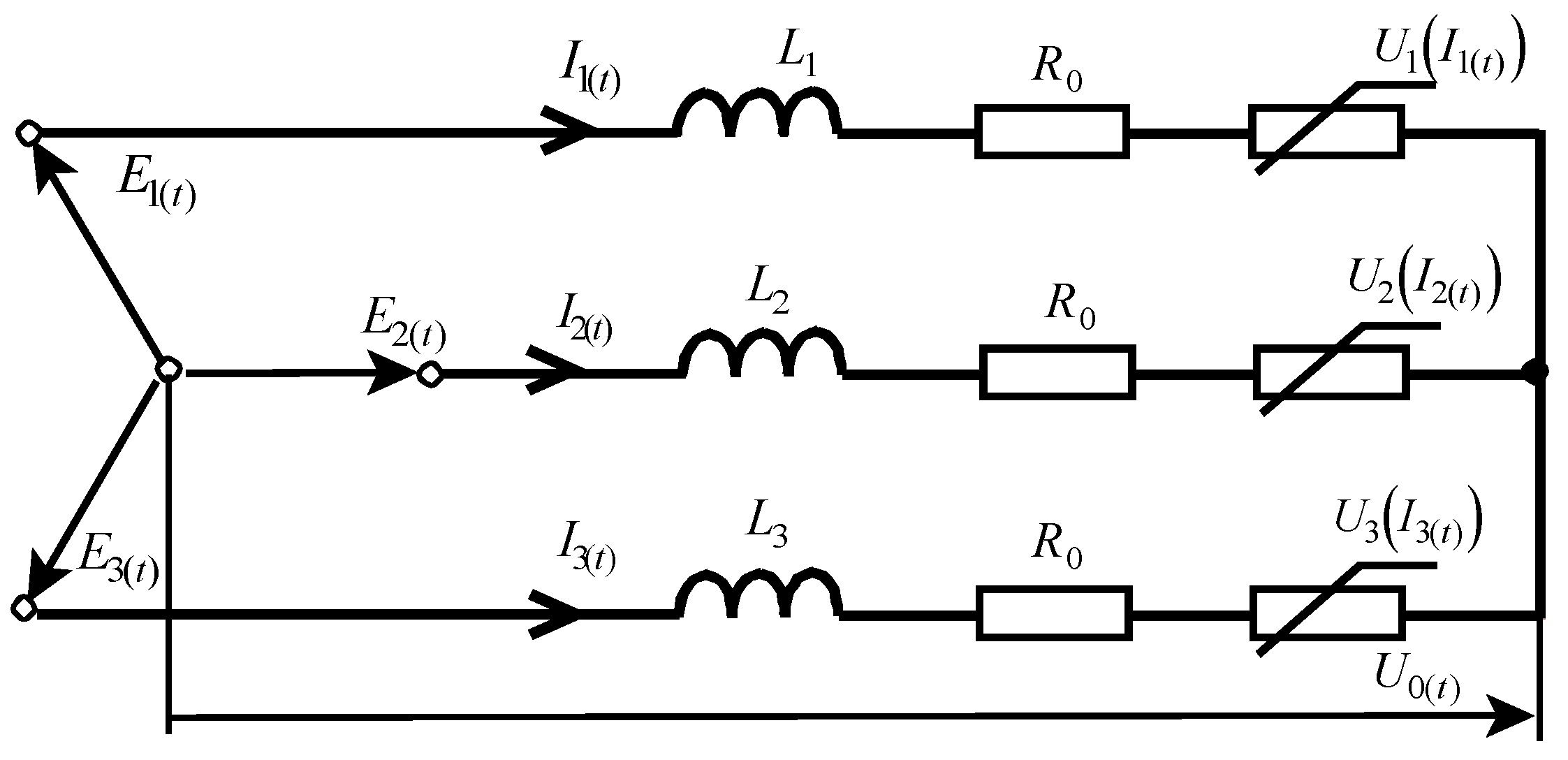
Based on the connection diagram of three-phase loads such as e.g., arc furnaces, an equivalent diagram of a three-phase circuit with a non-linear load is adopted, as shown in Figure 1. This diagram includes inductors and resistors that represent the behaviour of components found in the power system, such as transformers, transmission lines, and equivalent impedance introduced by the load. Also equivalent in nature are the AC voltage sources, which have the same frequencies and are mutually shifted in phase by 2π/3 and 4π/3 but have different amplitudes.

It was assumed that the load voltage in each phase can be described as the product of an arc-length-dependent parameter and an odd function of the phase current:

$$U_k(t) = H_{k}f(I_k(t)), H_k>0,k=1,2,3$$

(1)

One possible case of this function is the signum function, which was first used in [21]. The equations describing the circuit in Figure 1 are as follows:

$$L_k{\dot{I}}_k(t)+R_k{I}_k(t)+U_k\left(I_k(t)\right)+U_0(t)=E_k(t)$$

(2)

where:

$$E_k(t)=E_s\sin \left(\omega t+\left(k-1\right)2\pi /3+\psi \right)$$

(3)

The circuit under consideration is a three-phase circuit without a neutral conductor. This means that:

$$I_1(t)+I_2(t)+I_3(t)=0$$

(4)

For a non-linear load U₀(t), the voltage between the zero (centre) points of the load star and the star of the sinusoidal supply voltages is equal to:

$$U_0(t)=\frac{1}{3}{\displaystyle \sum _{k=1}^3\left(E_k(t)-L_k{\dot{I}}_k(t)-R_k{I}_k(t)\right)}-\frac{1}{3}{\displaystyle \sum _{k=1}^3{U}_k\left(I_k(t)\right)}$$

(5)

In a steady state, the voltage U₀(t) has two components: one dependent on the symmetry of the supply part and one dependent on the symmetry of the load. For equal phase amplitudes of the supply voltages, equal inductance, resistance and H-parameters of the load voltages (1), the system is balanced, and the first component is zero. The second component and thus the voltage U₀(t) are non-zero. For the arc voltages described by the signum function of the current, the voltage U₀(t) is a rectangular wave with three times less amplitude than the arc voltages and three times higher frequency. In IEC 60676 [22], only the first component (5) is considered.

The circuit Is described by state variables. In this case, these are the phase currents. In steady state, the phase currents can be written in general form as follows:

$$I=I\left(E,R,L,H,U_o,\omega \right)$$

(6)

where:

$$I=\left[\begin{array}{c}{I}_1\\ I_2\\ I_3\end{array}\right], E=\left[\begin{array}{c}{E}_1\\ E_2\\ E_3\end{array}\right], R=\left[\begin{array}{c}{R}_1\\ R_2\\ R_3\end{array}\right], L=\left[\begin{array}{c}{L}_1\\ L_2\\ L_3\end{array}\right], H=\left[\begin{array}{c}{H}_1\\ H_2\\ H_3\end{array}\right]$$

(7)

The elements I_k and E_k denote the amplitudes of the current and supply voltage in the k-th phase, respectively. The values of the elements of the above vectors are different in general, but the highest load power and energy delivery efficiency are obtained when they are equal to each other. Therefore, it is assumed that the individual vectors can be written in the form of currents:

$$I=\left[\begin{array}{c}{I}_s\\ I_s\\ I_s\end{array}\right]+\left[\begin{array}{c}{I}_1-I_s\\ I_2-I_s\\ I_3-I_s\end{array}\right]=I_s·\left[\begin{array}{c}1\\ 1\\ 1\end{array}\right]+\left[\begin{array}{c}\Delta I_1\\ \Delta I_2\\ \Delta I_3\end{array}\right]=I_s·1+\Delta I$$

(8)

The variable I_s is chosen so that the sum ${\Delta I_1}^2+{\Delta I_2}^2+{\Delta I_3}^2$ is as small as possible. This condition is met when:

$$I_s=\left(I_1+I_2+I_3\right)/3$$

(9)

Furthermore, it is assumed that:

$$\Delta I_k=I_s·O(\epsilon ), \epsilon =o(1), \mathrm{for}k=1,2,3$$

(10)

The values E_s, R_s, L_s and H_s are selected similarly. The latter parameter determines the phase voltages of the load. It is also assumed that the different component vectors of the other vectors satisfy a relation analogous to (10). By substituting the expansions of the remaining vectors similar to (8) and developing (6) into a Taylor series and later omitting the terms of order ε, one obtains:

$$I=I\left(E_s·1+\Delta E,R_s·1+\Delta R,L_s·1+\Delta L,H_s·1+\Delta H,\omega \right)=I\left(E_s·1,R_s·1,L_s·1,H_s·1,\omega \right)+O\left(\epsilon \right)$$

(11)

The above expression describes only the current’s vector determined for equal phase parameters of the circuit, i.e., for a balanced circuit.

3. Steady-State Analysis of a Three-Phase Balanced Circuit, Symbolic Solution

A three-phase balanced circuit in which the load voltage is denoted by H_s = U_a was considered in [21,23]. It was further assumed that the voltage of a non-linear load is described by the relation:

$$U_k(t)=U\left(I_k(t)\right)=U_a·\mathrm{sign}\left(I_k(t)\right)=\left\{\begin{array}{c}\begin{array}{cc}{U}_a& I_k(t)>0\end{array}\\ \begin{array}{cc}0& I_k(t)=0\end{array}\\ \begin{array}{cc}-U_a& I_k(t)<0\end{array}\end{array}\right.; U_a>0$$

(12)

In this model, the voltage is a balanced rectangular wave with amplitude U_a and frequency equal to the frequency of the power source. The voltages in the individual phases of the circuit are shifted in time by angles 2π/3 and 4π/3. As a result, the voltage U₀(t) is a rectangular wave with amplitude U_a/3 and angular frequency 3∙ω, and the circuit can be represented as three single-phase circuits whose currents and voltages are shifted in time by angles 2π/3 and 4π/3, the load voltages being described by the sum of U_ak(t) + U₀(t), where:

$$U_0(t)=-\left(U_1(t)+U_2(t)+U_3(t)\right)/3$$

(13)

Using time scaling:

$$\tau =\omega ·t$$

(14)

and dimensionless variables:

$$u_a=\frac{U_a}{E_s}; r_o=\frac{R_s}{\omega L_s}; u_{k\left(t\right)}=\frac{U_{k\left(t\right)}}{E_s}; u_{0\left(t\right)}=\frac{U_{0\left(t\right)}}{E_s}; i_{k\left(t\right)}=\frac{I_{k\left(t\right)}}{I_r}; I_r=\frac{E_s}{\omega L_s}$$

(15)

Equation (2) of phase 1 ($k=1$) of a balanced circuit can be represented as:

$$\frac{d{i}_1(\tau )}{d\tau }+r_o{i}_1(\tau )+u_1(\tau )+u_0(\tau )=\sin \left(\tau +\psi \right)$$

(16)

For the non-linear load described by Equation (12) at steady state, over a certain range, the voltage is a symmetrical rectangular wave with amplitude and fundamental harmonic angular frequency equal to 1, and the phase currents flow without interruption. This voltage can be represented as a Fourier series:

$$u_1(\tau )=u_{1h1}·{\displaystyle \sum _{n=1}^{\infty }\frac{1}{2n-1}·\sin \left(\left(2n-1\right)\tau \right)}; u_{1h1}=\frac{4u_a}{\pi }$$

(17)

As previously mentioned, the voltage u₀(τ) is a symmetrical rectangular wave with amplitude u_a/3, harmonic pulsation equal to 3 and can be represented as a Fourier series:

$$u_0(\tau )=-u_{1h1}·{\displaystyle \sum _{n=1}^{\infty }\frac{1}{3·\left(2n-1\right)}·\sin \left(3·\left(2n-1\right)\tau \right)}=-\frac{u_{1h1}}{3}·{\displaystyle \sum _{n=1}^{\infty }\frac{1}{\left(2n-1\right)}·\sin \left(3·\left(2n-1\right)\tau \right)}$$

(18)

The Fourier series of voltages u₁(τ) and u₀(τ) contain only odd harmonics. Whereby all harmonics u₀(τ) occur in the u₁(τ) harmonics spectrum. They have exactly the same frequencies and amplitudes but are shifted in phase by 180°. This means that in Equation (16), triple harmonics will not occur.

The phase shift angle ψ between the supply voltages and the first harmonics of the load voltages in (16) was introduced to facilitate further analysis.

Analysing the current, the solution of Equation (16) after substituting (17) and (18) at steady state (quasi-static) according to [24], two components can be distinguished: the fundamental harmonic and the sum of the higher harmonics:

$$i_1(\tau )=i_{1h1} ·\sin \left(\tau +{\varphi }_1\right)+{\displaystyle \sum _{\nu }{i}_{1h\nu }·\sin \left(\nu ·\tau +{\varphi }_{\nu }\right)}$$

(19)

where:

$$\nu =\left(\left(2n-1\right)\ne m·3\right) \mathrm{dla} n\in 〈2,3,\left.\dots \right),m\in 〈1,2,\left.\dots \right)$$

(20)

From the definition of the load characteristics, for $\tau =k\pi$; $k=0, 1, 2,\dots$ from (12) follows the relation:

$${\displaystyle \sum _{n=1}^{\infty }{i}_{1h\left(2n-1\right)}·\sin \left({\varphi }_{\left(2n-1\right)}\right)=0}$$

(21)

which can be written in a slightly different form:

$$i_{1h1}·\sin \left({\varphi }_1\right)=-{\displaystyle \sum _{\nu }{i}_{1h\nu }·\sin \left({\varphi }_{\nu }\right)}$$

(22)

Applying trigonometric transformations and separating the factors occurring at $\cos \left(\left(2n-1\right)\tau \right)$ and $\sin \left(\left(2n-1\right)\tau \right)$ for n > 1, one obtains:

$$i_{1h\left(2n-1\right)}=\frac{u_{1h1}}{\left(2n-1\right)·\sqrt{{\left(2n-1\right)}^2+r_o^2}}; \sin \left({\varphi }_{\left(2n-1\right)}\right)=\frac{\left(2n-1\right)}{\sqrt{{\left(2n-1\right)}^2+r_o^2}}$$

(23)

Hence, after taking into account that r_o follows:

$${\displaystyle \sum _{\nu }{i}_{1h\nu }·\sin \left({\varphi }_{\nu }\right)}={\displaystyle \sum _{\nu }\frac{u_{1h1}}{{\nu }^2+r_o^2}}\cong u_{1h1}{\displaystyle \sum _{\nu }\left(\frac{1}{{\nu }^2}-\frac{r_o^2}{{\nu }^4}\right)}$$

(24)

In [25] it can be found the following infinite sums:

$${\displaystyle \sum _{n=1}^{\infty }\frac{1}{n^2}}=\frac{{\pi }^2}{6}; {\displaystyle \sum _{n=1}^{\infty }\frac{1}{n^4}}=\frac{{\pi }^4}{90}; {\displaystyle \sum _{n=1}^{\infty }\frac{1}{n^6}}=\frac{{\pi }^6}{945}$$

(25)

Taking into account that only the higher odd harmonics are summed, and with a frequency that is not a multiple of the triple of the fundamental harmonic frequency, the relation can be estimated:

$$i_{1h1}·\sin \left({\varphi }_1\right)=-\frac{4u_a}{\pi }{W}_T$$

(26)

where:

$$W_T=\left(\frac{{\pi }^2}{9}-1\right)-r_o^2\left(\frac{5{\pi }^4}{486}-1\right)\cong 0.0966-0.00215r_o^2$$

(27)

It follows from relations (26) and (27) that the fundamental harmonic of the current is lagged with respect to the fundamental harmonic of the load voltage.

Similarly, the square of the root mean square (RMS) value of the higher harmonic currents can be calculated:

$$i_{1H}^2={\displaystyle \sum _{\nu }{i}_{1h\nu }^2}={\displaystyle \sum _{\nu }\frac{u_{1h1}^2}{{\nu }^2\left({\nu }^2+r_o^2\right)}}\cong u_{1h1}^2{\displaystyle \sum _{\nu }\left(\frac{1}{{\nu }^4}-\frac{r_o^2}{{\nu }^6}\right)}$$

(28)

$$i_{1H}^2\cong u_{1h1}^2\left(\frac{5{\pi }^4}{486}-1-r_o^2\left(\frac{22{\pi }^6}{21149}-1\right)\right)=u_{1h1}^2\left(0.00215-r_o^{2}0.0000734\right)$$

(29)

For comparison, the square of the RMS value of the equivalent higher harmonics of the load voltage is:

$${\left(u_1(\tau )+u_0(\tau )\right)}_{1H}^2={\displaystyle \sum _{\nu }{\left(u_1(\tau )+u_0(\tau )\right)}_{1h\nu }^2}=u_{1h1}^2{\displaystyle \sum _{\nu }\frac{1}{{\nu }^4}}=0.0966 u_{1h1}^2$$

(30)

The equivalent load phase voltage in a three-phase balanced circuit is given by:

$$\left(u_1(\tau )+u_0(\tau )\right)=u_z$$

(31)

The amplitude of the fundamental harmonic of the equivalent load voltage u_z in phase 1 is equal to the fundamental harmonic of the voltage u₁(τ) and is u_1h1 (17). However, the harmonic content coefficients differ:

$$THD{u}_1=\sqrt{{\displaystyle \sum _{n=2}^{\infty }\frac{1}{{\left(2n-1\right)}^2}}}=\sqrt{\frac{{\pi }^2}{8}-1}=\sqrt{0.237}=0.4834$$

(32)

$$THD{u}_z=\sqrt{{\displaystyle \sum _{n=2}^{\infty }\frac{1}{{\left(2n-1\right)}^2}}-\frac{1}{9}{\displaystyle \sum _{n=1}^{\infty }\frac{1}{{\left(2n-1\right)}^2}}}=\sqrt{\frac{{\pi }^2}{9}-1}=\sqrt{0.0966}=0.310;$$

(33)

Based on the balance of the fundamental harmonic [16], the relation was obtained:

$$i_{1h1}=\sqrt{{\left[\frac{1}{1+r_o^2}\left(\sqrt{1 + r_o^2-{\left(u_{1h1} \left(1+W_T\left(1+r_o^2\right)\right)\right)}^2}-u_{1h1}{r}_o\right)\right]}^2 +{\left(u_{1h1}{W}_T\right)}^2}$$

(34)

Hence, the current harmonic content factor has the form:

$$TH{D}_i\cong \frac{u_{1h1}}{i_{1h1}}0.0464(1-{r_o}^{2}0.017)$$

(35)

The harmonic content coefficient of a non-linear load voltage is defined by (32).

Equation (26) means that the phase shift angle between the first harmonic of the current and the load voltage is negative, indicating that the current lags behind the voltage. Therefore, for the fundamental harmonic, the series equivalent diagram of a nonlinear element consists of inductance and resistance. In further analysis, an equivalent circuit diagram in the form of a series of connected elements is useful. Based on the voltage drops across these elements and (26), equivalent element values can be calculated:

$$\omega L_Z=\omega L\frac{u_{1h1}}{i_{1h1}}\sin ({\varphi }_1)=\omega L{\left(\frac{u_{1h1}}{i_{1h1}}\right)}^2{W}_T(r_o)$$

(36)

$$R_Z·=\omega L\frac{u_{1h1}}{i_{1h1}}\cos ({\varphi }_1)\cong \omega L\frac{u_{1h1}}{i_{1h1}}\left(1-0.5{\left(\frac{u_{1h1}}{i_{1h1}}·W_T(r_o)\right)}^2\right)$$

(37)

Especially interesting is the relation (36). The considered load described by an odd and unambiguous nonlinear function has an inductance in the equivalent diagram, that is, a conservative element with an ambiguous current-voltage characteristic. However, the nonlinear element acts as a voltage source for higher harmonics, with the amplitudes and phase shifts of currents being determined by the L_s and R_o elements of the circuit, satisfying the relation (22). As a result, an increase in the circuit’s inductance is observed for the fundamental harmonic.

The characteristics and equivalent parameters of the circuit are analysed as functions of u_a and r_o. Due to the required energy efficiency of the three-phase arc furnace circuit, the study was conducted for r_o ≤ 0.3. The relations presented above refer to the uninterruptible current flow that occurs for 0 < u_a < u_b, where u_b is the smallest value of u_a, at which, for a certain τ, the value of the equivalent load voltage is equal to the value of the supply voltage. For a balanced three-phase system with a phase resistance described by r_o = 0, this limiting value of u_a is:

$$u_b=\frac{3/2}{\sqrt{1+{\left(\raisebox{1ex}{$2\pi $}\!\left/ \!\raisebox{-1ex}{$3$}\right.\right)}^2}}=0.646$$

(38)

As r_o increases, the value of u_b decreases slightly. Analysing the circuit model, it was found that for u_a = 0.75, the amplitude of the equivalent voltage u_z is equal to 1 and that, for u_a = 0.80, the amplitude of the dimensionless current is about 0.05. Therefore, the study was carried out for 0.1 < u_a ≤ 0.8. But the obtained relations are valid for u_a < 0.646. To study the effect of the circuit resistance, i.e., the parameter r_o, and how the results will look for larger values of u_a, the circuit from Figure 1 was simulated in Simulink.

4. Simulation of a Circuit Model with a Non-Linear Load

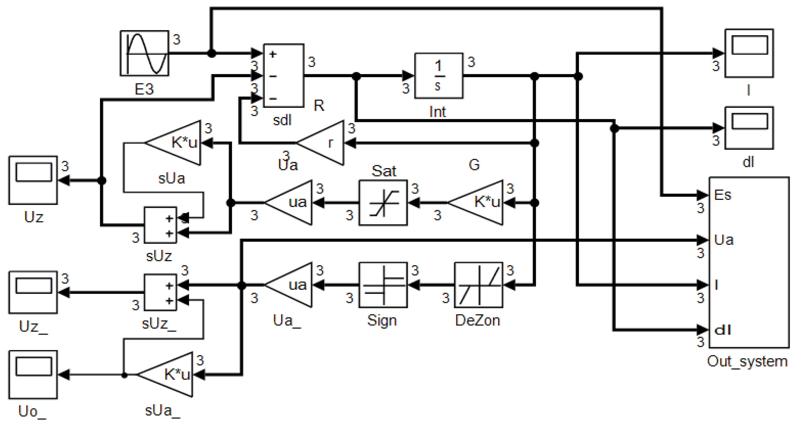
A three-phase circuit supplied from a sinusoidal three-phase voltage source is considered, containing an inductance and resistance in series with a non-linear element equal in each phase. For simulation purposes, the circuit depicted in Figure 1 was modelled in Simulink, as shown in Figure 2.

This diagram uses the possibility of implementing vector block operators. The connections shown in bold line refer to vectors of phase signals of the same type. The indices of the vectors denote the magnitudes of the individual phases of the circuit, as can be seen in (3).

The linear part of Equation (2) was realised on an sDI summator, an Int integrator and an R amplifier. The non-linearity defined by the signum function—Equation (1) led to computational issues, resulting in system hang-ups when variable-step methods for solving ordinary differential equations were employed. As a solution, the nonlinear load system was represented by a saturation block with a high gain (10⁴) for the linear portion of the characteristic. Saturation levels were proportional to the amplitude of the non-linear receiver voltages u_a. Based on the signals, the voltage u₀ is created as one-third of the summed phase voltages of load. The voltage u₀ is output of block labelled as sUa in Figure 2. The outputs sUa and vector of ua voltages result in an equivalent load voltage sUz. In such a system, the load characteristic in the form (1) is directly not observed. It can be noted that when the load voltage is close to the supply voltage, the current is close to zero. The reactive power of the load determined from this voltage can be misleading. Therefore, the diagram of Figure 2 contains additional blocks modelling a non-linear load whose characteristics are described by (1). Among these blocks is the DeZon (Dead Zone) block. The parameters r_o and u_a for a balanced system are scalars.

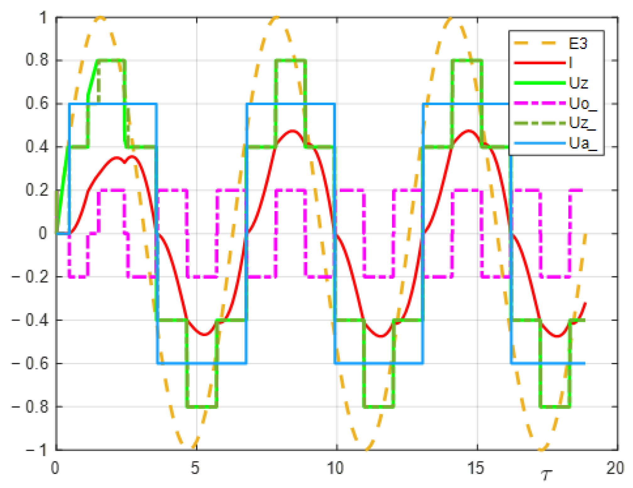
In Figure 3, the time-domain plots depict the dimensionless variables of the supply voltage, current derivative, current, and load voltage. These waveforms correspond to a nonlinear load with a voltage amplitude of u_a = 0.6 and a resistance r = 0.1.

When either of the phase currents is close to zero, there are differences between the voltages Uz and Uz_—Figure 3. These differences depend on the ODE solution method used. Following an analysis of the current waveform across different solution methods, the RK23 solver was ultimately applied. In the magnification, the near-zero current has the character of a relaxation oscillation, while the voltage of the non-linear element at this time section coincides with the supply voltage, i.e., the voltage drop across the inductance and resistance is close to zero. In order to obtain a voltage corresponding to model (1), an additional system for observing the load voltage was used, and its operation can be seen in the diagram.

The operating diagram in Figure 2 facilitates the observation of the instantaneous values of currents and voltages of the circuit in Figure 1. The steady-state uses the quantities characterising these quantities averaged over a period. That analysis of the earlier presented circuit divides the procedure into two stages: analysing the higher harmonics and subsequently analysing the fundamental harmonic. To execute this procedure numerically, the sine and cosine components of the fundamental harmonic, along with the mean value of the square of the instantaneous current, which equals the sum of the squares of the amplitudes of all harmonics, are determined within the output system.

$$\begin{array}{l}{i}_s=\frac{1}{\pi }{\displaystyle {\int }_0^{2\pi }i(\tau )}·\sin (\tau )·d\tau \\ i_c=\frac{1}{\pi }{\displaystyle {\int }_0^{2\pi }i(\tau )}·\cos (\tau )·d\tau \end{array}$$

(39)

$$i_{ms}^2=\frac{1}{\pi }{\displaystyle {\int }_0^{2\pi }i{(\tau )}^2}·d\tau$$

(40)

The time functions sin(τ) and cos(τ) used in these calculations are generated in a separate block. An exemplary scheme for determining the sin/cos components of the variable i(τ)—input In1 is shown in Figure 4. The functions sin(τ) and cos(τ) are input to vIn2.

At the output of the multiplication system, a vector of subintegral functions is obtained. Further computations are conducted for consecutive intervals and are synchronised via the sin(τ) signal (commencement of each period of the supply voltage) on integrators denoted as Int_1 and Int_2. Int_1 has to be configurated External reset as rising, Int_2 External reset as rising and Initial condition source as external. The former integrates the output signal (signal vector) derived from the multiplication system denoted as Pr_1, where inputs are furnished with an instantaneous quantity (e.g., current) and a vector of sin(τ) and cos(τ) waveforms. Before the start of a new period, the value of the Int_1 output integral is remembered in the Mem block and in the new period, it is passed to Int_2, whose output is divided by π and completes the averaging operation. The vector of sine and cosine components of the current (as (39)) is obtained at the output (outport Out).

When identical signals are applied to the inputs of the multiplication system (such as instantaneous current), the output yields the doubled average square of the root mean square (RMS) value, effectively representing the sum of the squares of the harmonic amplitudes.

In this way, a system was modelled to measure the sine, cosine and double square of the RMS value of the current, load and supply voltages. By subtracting the square of the RMS value of the current from the square of the base harmonic amplitude, the sum of the squares of the higher harmonic amplitudes is obtained, which is then called the square of the higher harmonic amplitudes [24]:

$${i_H}^2={\displaystyle \sum _{k=2}^{\infty }({i_k}^2})={i_{ms}}^2-{i_s}^2-{i_c}^2$$

(41)

The mentioned connections facilitate the calculation of ratios of harmonic content, the active power of circuit voltages and currents, and the values of equivalent circuit components. Consequently, this method allows for the computation of the supply voltage, voltage and current of non-linear loads, as well as the active and reactive power of fundamental harmonics and higher harmonics within the circuit.

5. Characteristics of a Model of a Three-Phase Balanced Circuit with a Non-Linear Load

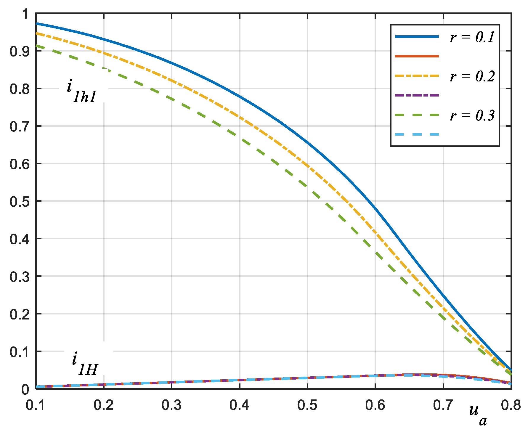
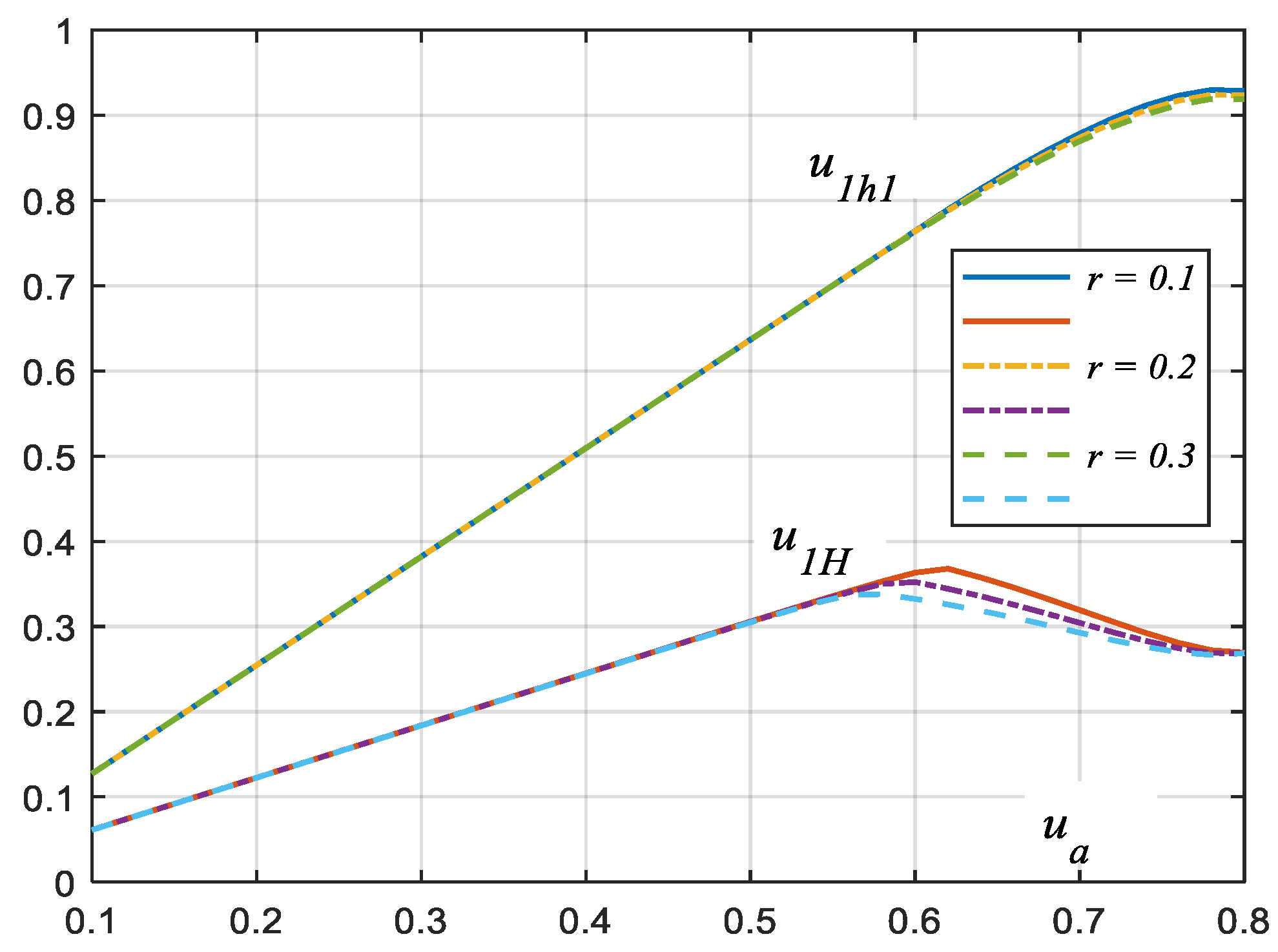
The simulation experiment was managed through a MATLAB program. Computations were conducted across 10 intervals of the supply voltage, where the voltage u_a ranged from 0.1 to 0.8, with varying values of r set at 0.1, 0.2, and 0.3. The obtained results were related to those of the single-phase circuit presented in [17]. On the basis of the current waveforms for u_a > 0.8, it was found that the amplitude of the dimensionless current is less than 5%, and the tested circuit is not efficient. The characteristics of the amplitude of the higher harmonics and the fundamental harmonic of the current are shown in Figure 5.

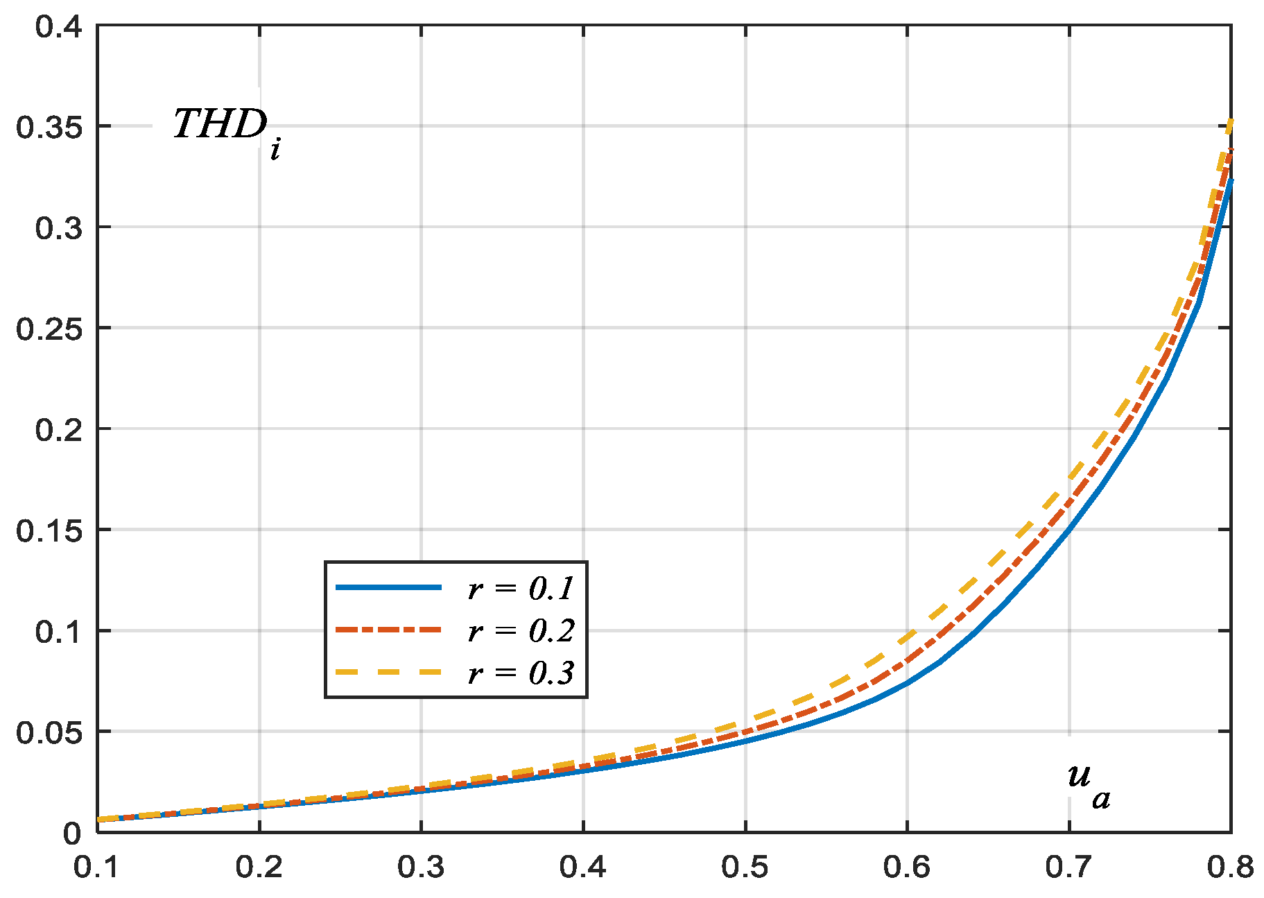
The graphs in Figure 5 show that the higher harmonic content of the current is approx. 3-fold lower for a three-phase circuit than for a single-phase circuit [17]. For u_a ≈ 0.6, the amplitude curves of the first harmonic have inflexion points, and as u_a increases further, they converge and tend towards zero. The same is true for the higher harmonics. As a result, an increase in the ratio of the higher harmonic content of the current in the circuit under consideration is observed—Figure 6.

Coefficient THD_i is not specified in the IEEE 519 standard [15]. Instead, TDD (total demand distortion) is introduced, which can be translated as total desired distortion. For a fairly stiff power system (the rms value of the short-circuit current is greater than one hundred rms values of the load current), in the band up to the 50th harmonic, the TDD factor should be less than 12%. Assuming such a limitation for THD_i, Figure 6 shows that, for u_a = 0.63, this ratio exceeds the value described in the IEEE 519 standard [15] and increases quite rapidly with the value of u_a. A slightly different character is found in the frequency spectrum of the load voltage. The characteristics of the amplitudes of the higher harmonics and the fundamental harmonic of this voltage are shown in Figure 7.

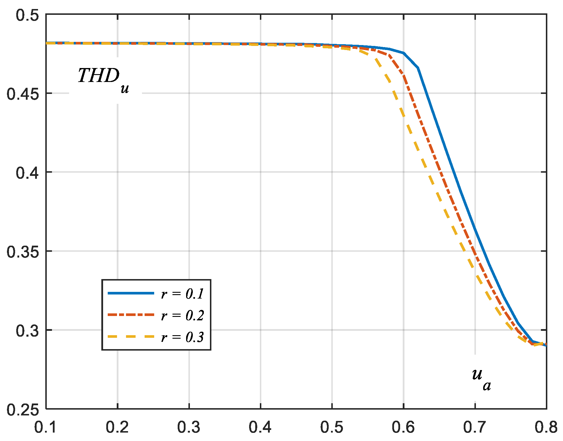
For u_a < 0.6, the graphs in Figure 7 can be considered linear. This is due to the constancy of the shape of the voltage waveform and its independence from the current. For the single-phase model [9], the voltage limit is lower and is approximately 0.5. The association between the higher harmonics and the fundamental harmonic of the load voltage is established through THD_u. This relationship is illustrated in Figure 8, where THD_u is depicted as a function of u_a and r.

In this graph, the value of THD_u for u_a < u_b is constant and independent of r. Only when u_a exceeds this value does THD_u decrease by almost twice. The minimum THD_u occurs for u_a ≈ 0.8.

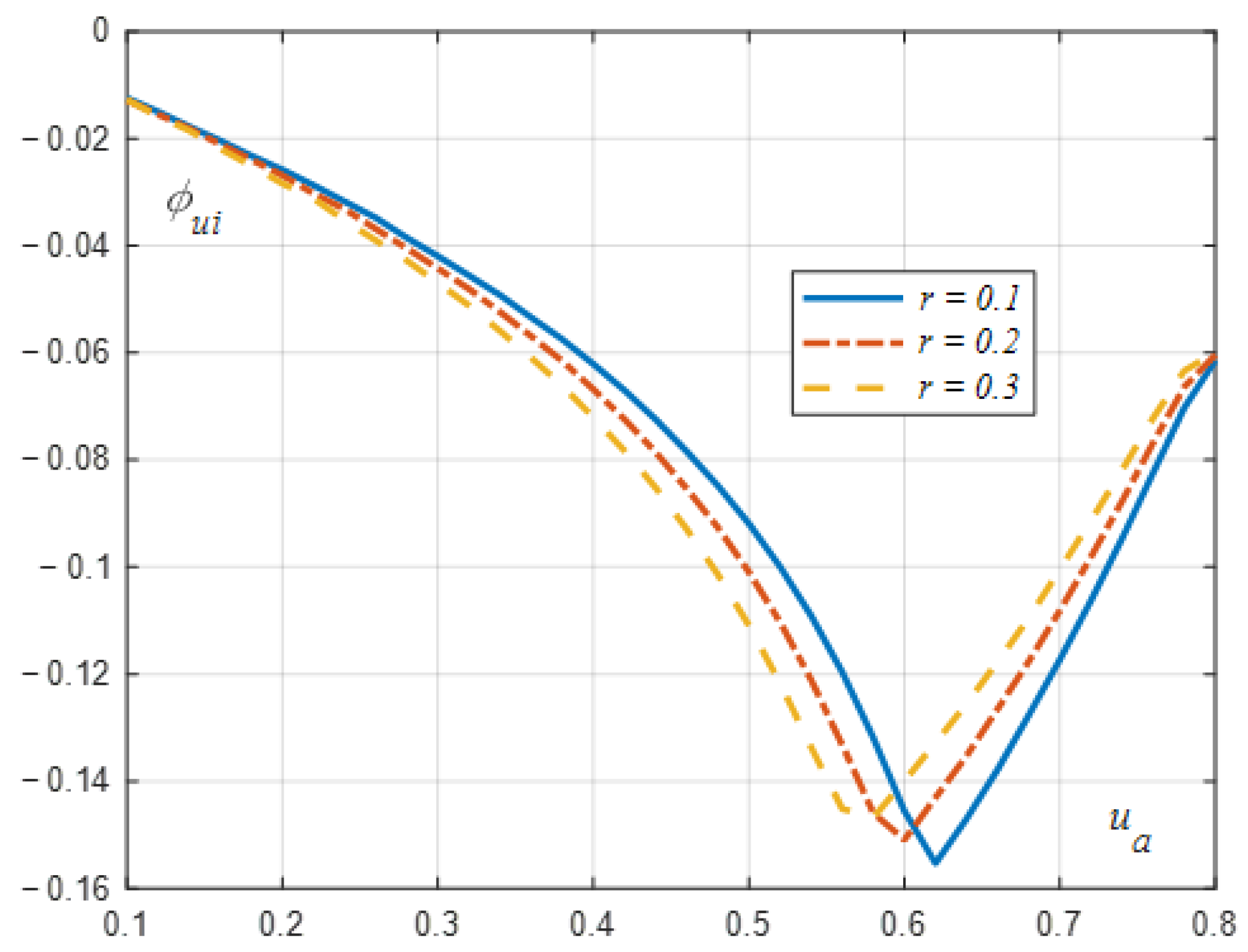
The Total Harmonic Distortion (THD) coefficients solely establish the connection between the amplitudes of currents and voltages within the fundamental harmonic circuit and the higher harmonic circuit. Energy transmission occurs from the voltage source to the resistance and non-linear load, primarily through the first harmonic of the current. The intensity of the current is contingent upon the characteristics of the load as perceived by the source. To identify this characteristic, it is crucial to ascertain the phase shift angle (ϕ_ui) between the current and voltage of the non-linear load. This angle is defined as the variance between the phase angles of the first harmonics of the load’s voltage and current concerning the voltage of the power source. Figure 9 illustrates a graph depicting the phase shift of the load (ϕ_ui).

The angle ϕ_ui is negative and has a minimum value equal to about −0.15 radians for u_a = u_b (38), for the maximum value of the load voltage amplitude at the load of the uninterruptible current flow. For a single-phase system, the value is lower and equal to approx. −0.24 radians. For uninterruptible current flow, the minimum value ϕ_ui increases slightly with the value of r. Associated with the negative phase shift is the inductance in the equivalent diagram of the non-linearity. The phase shift of the current with respect to the load voltage for u_a > u_b tends to zero as u_a increases. The values of the elements of the equivalent diagram of the nonlinear load are also determined by the amplitude of the fundamental harmonic of the current, which for u_a > u_b decreases quite rapidly with u_a. Therefore, the elements of the equivalent diagram (including the equivalent inductance) were determined on the basis of this phase shift of the current with respect to the supply voltage and the amplitudes of the fundamental harmonic of the current and the supply voltage.

Considering that energy flow in the analysed circuit is associated with the fundamental harmonic, the power factor is calculated as the cosine of the phase shift angle between the fundamental harmonic of the current and the fundamental harmonic of the supply voltage. A plot of the power factor of the circuit as a function of the non-linear load voltage and resistance is shown in Figure 10.

In the u_a domain, the power factor diagrams show two distinct regions: a lower interval characterised by uninterrupted current waveform and an upper interval where interruptions in current flow occur alongside a rapid increase in the equivalent resistance of the non-linear load. This distinction is also visible in Figure 10, where for u_a > u_b, a noticeable decrease in the slope of the characteristic representing the phase shift angle of the fundamental harmonic of the current relative to the fundamental harmonic of the supply voltage can be observed.

The calculation of active power in the circuit involves averaging the product of current and voltage over time, following the configuration outlined in Figure 4. This calculation considers both the supply voltage and the load voltage. Figure 11 illustrates the phase powers associated with these voltages, varying with the load voltage amplitude and resistance (r).

$$p=\frac{1}{kT}{\displaystyle \underset{\tau }{\overset{\tau +kT}{\int }} u·i·dt}=\frac{P}{S_r}, S_r=\frac{{E_s}^2}{\omega L_s}$$

(42)

The three-phase circuit powers presented in dimensionless form are related to 3S_r.

It should be noted that the maximum power value occurs for uninterruptible current flow for u_a ≈ 0.48. This finding is important for the efficiency of power transfer in the circuit. Obviously, as the resistance r increases, the efficiency of the circuit decreases.

By analogy, the dimensionless reactive powers of the load and the entire circuit were estimated—Figure 12. These powers of the circuit were also related to 3S_r.

Following previous analyses [17], the concept of reactive power was defined as the result of multiplying voltage by the rate of change of current over time. This interpretation enables the calculation of reactive power’s instantaneous values and aligns with one of the formulations outlined in IEEE 1459-2010 [24] (p. 4).

$$Q=\frac{1}{\omega ·kT}{\displaystyle \underset{\theta }{\overset{\theta +kT}{\int }} u·\frac{di}{d\tau }·d\tau }=\frac{1}{2\pi }{\displaystyle \oint u·di}$$

(43)

The variable θ, which marks the onset of the averaging period, needs to be synchronised with the initiation of the supply voltage cycle. The latter part of this relationship serves as a rationale for a significant phenomenon. According to the adopted definition, the total reactive power of a non-linear load characterised by (1) equals zero, regardless of the load magnitude and circuit resistance. In other words, the combined reactive power of the fundamental harmonic and the higher harmonics equals zero, implying that the reactive power of the higher harmonics is equivalent to the negative reactive power of the fundamental harmonic, which is positive. This indicates that the non-linear load acts as the source of reactive power for the higher harmonics, allowing for the summation of reactive powers defined for both fundamental and higher harmonics.

This statement can be extended to non-linearities whose current-voltage characteristics are described by an odd function and are unambiguous (without hysteresis). The statement does not apply to reactive power calculated according to the IEEE algorithm.

The reactive power (43) may be presented in dimensionless form as follows:

$$q=\frac{1}{kT}{\displaystyle \underset{\theta }{\overset{\theta +kT}{\int }} u·\frac{di}{d\tau }·d\tau }=\frac{Q}{S_r}$$

(44)

For the adopted definition of reactive power, an important phenomenon was observed for both single-phase [17] and three-phase systems [23]. The total reactive power of a non-linear load with unambiguous q_N characteristics was very close to zero, but the reactive power calculated for the first harmonic q_N1 of this load was positive, different from zero. In contrast, the reactive power of the higher harmonics q_NH is negative; that is, the non-linear load is a source of the reactive power of the higher harmonics. The total reactive power of the circuit is denoted q_S.

In the circuit where higher harmonic currents flow, there exists nonlinearity—acting as the source of these higher harmonics—along with inductance and resistance. The voltage source supplying the fundamental harmonic behaves like a short circuit for the higher harmonics. Consequently, the reactive power associated with the higher harmonics is equivalent to the negative reactive power of the fundamental harmonic, which is positive. Thus, the non-linear load serves as the origin of reactive power for the higher harmonics. The reactive power of the non-linearity is taken from the power source and converted into reactive power of the higher harmonics, which is transferred to the inductance L_s of the circuit. Consequently, within the fundamental harmonic circuit, there’s an evident rise in the circuit’s inductance, denoted as Lc, ascertainable through the following correlation:

$$\frac{Lc}{L_s}=\frac{\left|e\right|}{\left|i_1\right|}·\sin \left(-{\varphi }_{ei}\right)=-\frac{1}{\left|i_1\right|}·\sin \left({\varphi }_{ei}\right)$$

(45)

This inductance is shown as a function of load voltage amplitude in Figure 13.

For u_a < 0.3, the equivalent inductance of the circuit closely approximates the inductance L, whereas for u_a ≈ 0.7, it reaches a value of 2L_s. This phenomenon of increasing circuit inductance was similarly observed for a non-linear load within a three-phase circuit in [16] and was experimentally verified by S. Köhle [26], who conducted measurements of arc furnace circuit parameters.

6. Conclusions

The analysed three-phase circuit with a load described by the signum function of the current is a rather special case in the power system [27,28]. But, as presented in section three, in a steady state, it is possible to solve the equations of this circuit symbolically (analytically), taking into account all higher harmonics. The analysis of this solution was used to verify the results of the circuit simulation (section four). Dimensionless variables made it possible to reduce and simplify the complexity of the system analysis and simulation of its model.

The load is also special. For continuous current flow, the phase load voltage is a rectangular wave, and its harmonic content is constant, depending only on the amplitude of this voltage. This makes it easier to analyse the distribution of active and reactive power in a circuit and to track the power of higher harmonics. Furthermore, it can be used to estimate the parameters (resistance and reactance) of a system feeding a non-linear load.

It should be emphasised that the characteristics of this circuit were determined symbolically and numerically with MATLAB-Simulink R2021b using vector operations. The results of both analysis methods are consistent.

For the considered load for u_a < 0.646 (r₀ = 0), the phase currents flows are continuous. For the considered condition, the harmonic content factor THDu in the load voltage is constant. It can be seen in Figure 8 that the smallest THDu occurs for u_a > 0.646 and u_a < 0.8. This finding has practical implications for choosing the circuit’s inductance, as it helps to reduce the adverse effects of the non-linear load on system performance and its impact on the power supply network.

Harmonic balance analysis in this study involved separate consideration of the fundamental harmonic circuit and the higher harmonic circuit, aligning with the principles outlined in the IEEE 1459 standard. This waveform analysis methodology, employed in this paper, draws upon techniques previously utilised in the measurement system described in [29]. It’s worth noting that the analysis methodology advocated by IEEE 1459 holds significant utility, serving purposes ranging from system analysis to the design of measurement systems or power quality monitoring tools.

From the analysis of the dependence of the active power on the load voltage amplitude of a non-linear load, it follows that the maximum value of the load active power occurs for u_a ≈ 0.5—Figure 11.

An important phenomenon is observed in the applied definition of reactive power—Figure 12. The total reactive power of the non-linear load is equal to zero. Such a result can be obtained from symbolic analysis. Such a phenomenon will occur for loads with odd current-voltage characteristics. This does not mean that the reactive power of the fundamental harmonic is zero. The reactive power associated with the fundamental harmonic is positively non-zero and is precisely equivalent to the negative power of the higher harmonics. The negative sign of the reactive power of the higher harmonics means that the non-linear load is the source of the higher harmonics. In the circuit under consideration, this power is being released in the inductance of the circuit. Hence, an important conclusion follows that the reactive power of the circuit calculated for the fundamental harmonic is equal to the reactive power of the circuit calculated, taking into account the higher harmonics. This phenomenon also occurs for active power. This means that the apparent power calculated from active and reactive power in both cases is also the same. But this is not valid for apparent power calculated from rms values of current and voltage.

The algorithm used in the work to determine reactive power as the product of the voltage and current time derivative simplifies the energy accounting process. It allows reactive energy to be measured in accordance with the requirements set out in the standard [30]. A reactive energy meter, according to this standard, should measure the reactive energy of the fundamental harmonic with minimal harmonic influence. The definition of reactive power utilised in the article, represented as the product of voltage and the time derivative of current fulfils this criterion.

The inductance of the circuit, as seen from the terminals of the power source, includes the inductive component of the circuit and the equivalent inductance of the nonlinear load for the fundamental harmonic. As the voltage amplitude of the nonlinear load increases, a significant increase in the phase circuit inductance for the fundamental harmonic is observed. For u_a = 0.7, it is a twofold increase, and for u_a = 0.8, an increase of up to five times. This increase in inductance is due to the non-linearity of the load. This increase also causes an increase in the fundamental harmonic of the reactive power of the circuit. This means that the non-linearity of the load causes an increase in reactive power.

Only selected characteristics of the analysed circuit are presented in this paper. The algorithms for determining the individual quantities can be used in real measurement systems [29]. Of course, they were implemented digitally.

The circuit considered in this paper may be a model of a three-phase arc furnace circuit during the beginning of melting.