
Artificial Intelligence-Centric Low-Enthalpy Geothermal Field Development Planning

 , ,
, ,
Abstract
1. Introduction
2. Conventional Field Development Planning
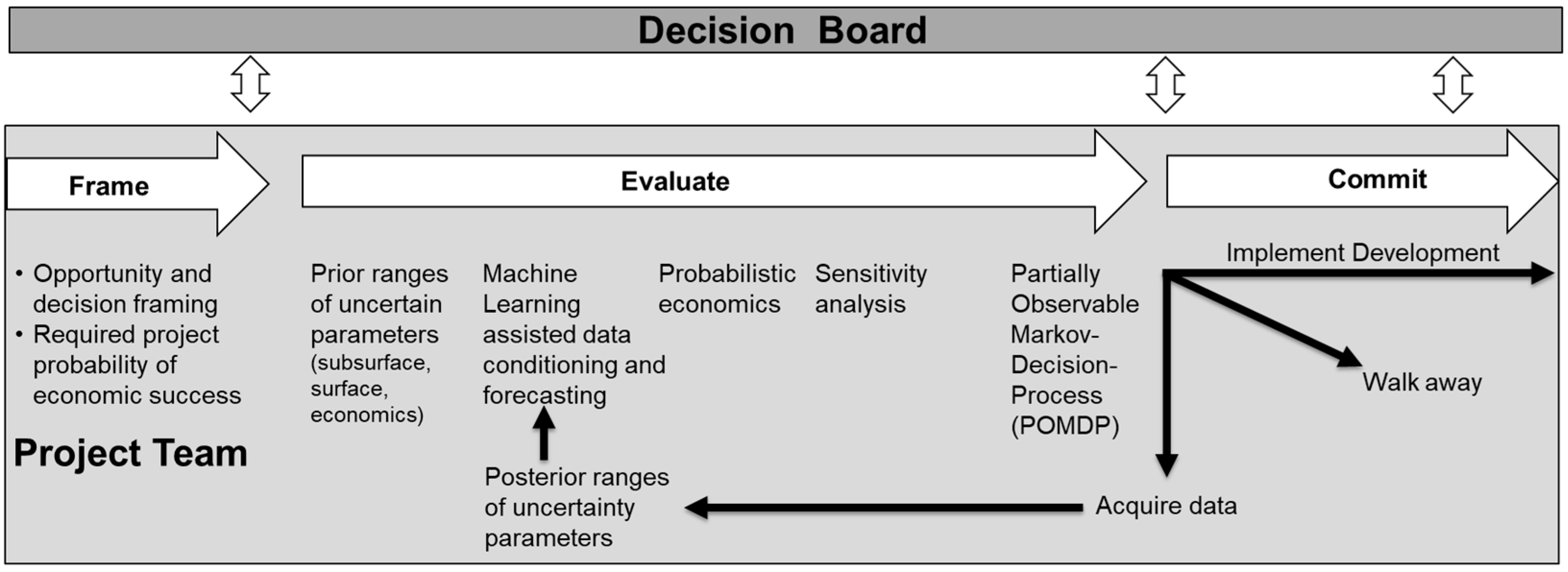
3. Artificial Intelligence-Centric Field Development Planning
3.1. Framing
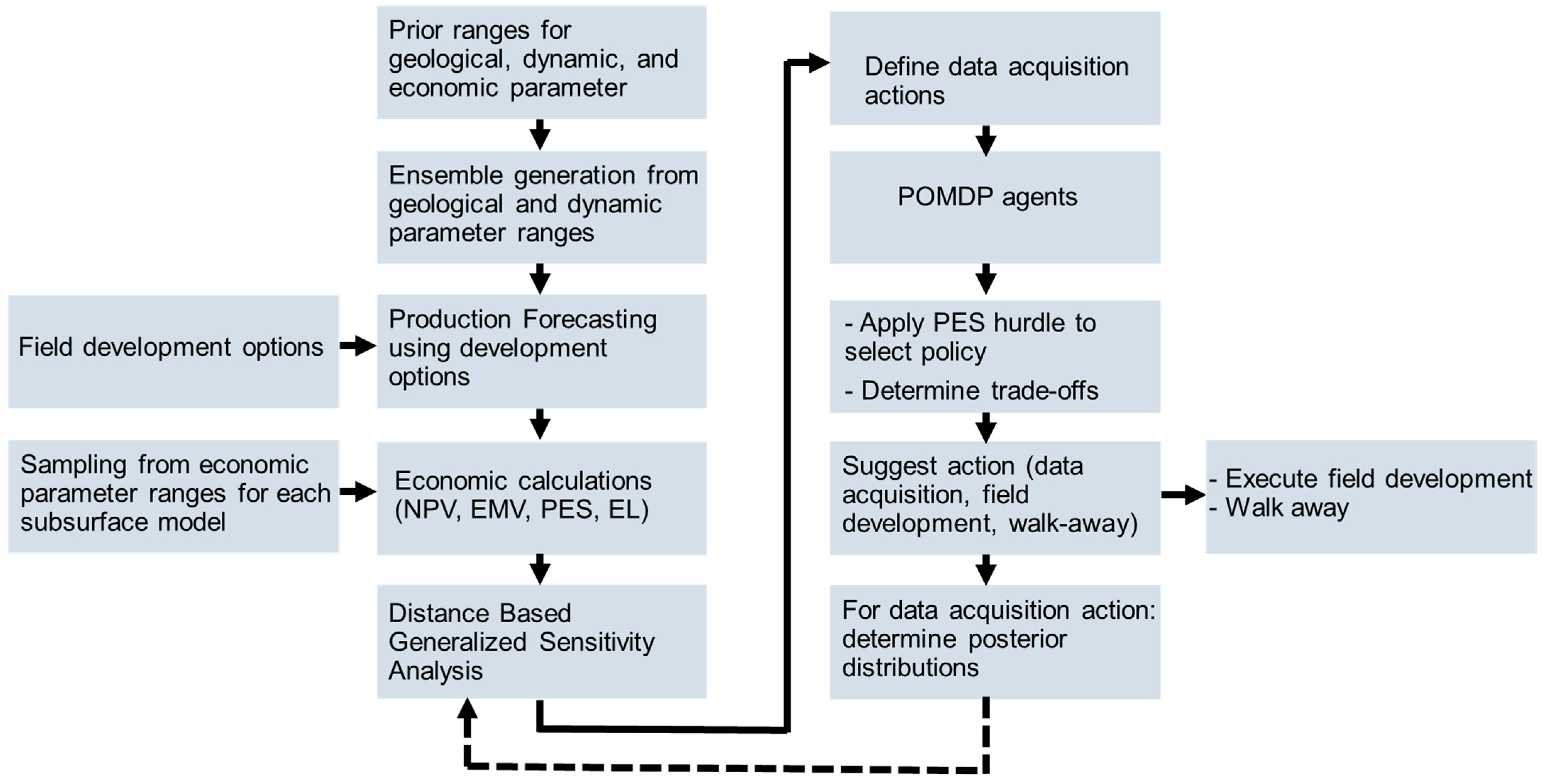
3.2. Evaluation
3.3. Commit
3.4. General Aspects
4. Case Study
4.1. Project Set-Up
4.2. Geothermal Reservoir Setting
4.3. Geological Reservoir Parameterisation
4.4. Dynamic Reservoir Parameterisation
4.5. Field Development Scenarios
4.6. Production Forecasts
4.7. Economic Parameters and Economic Analysis
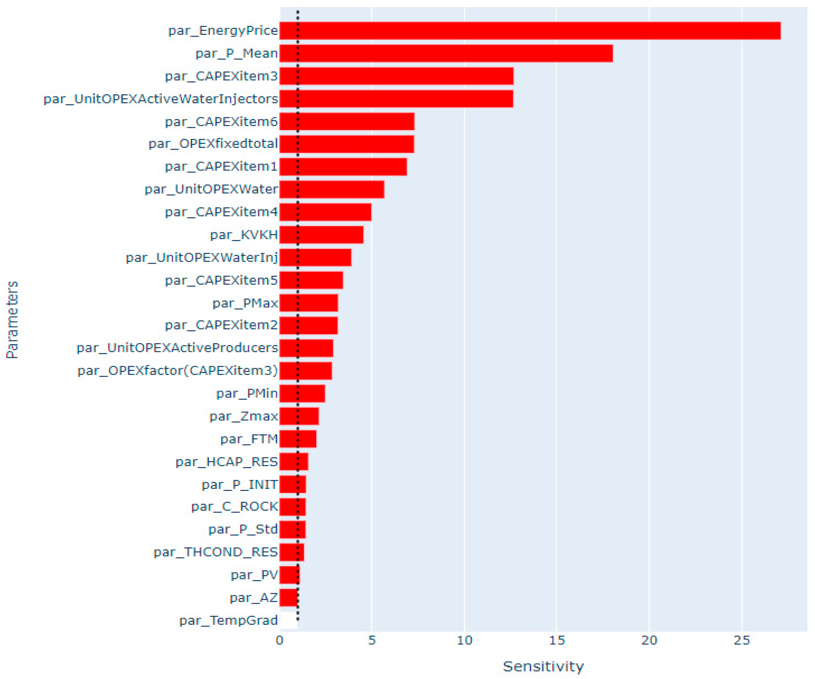
4.8. Sensitivity Analysis and Data Acquisition Actions
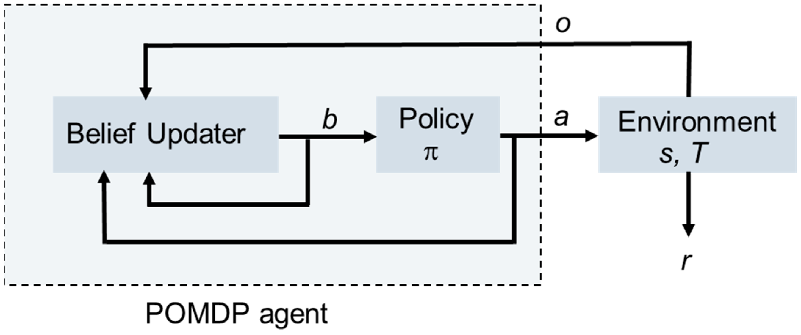
4.9. Partially Observable Markov Decision Process (POMDP)
4.9.1. Introduction of POMDP and Agent
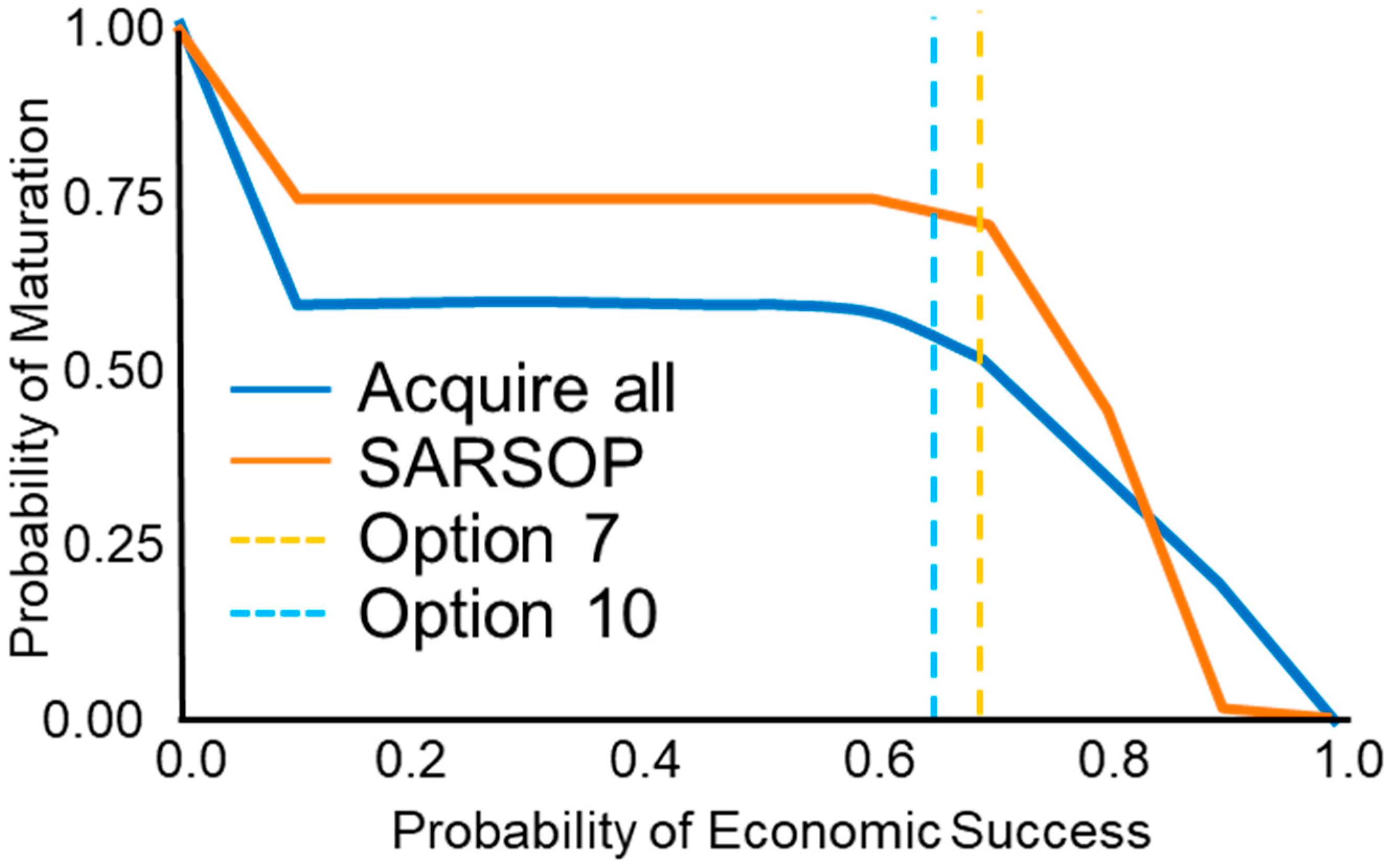
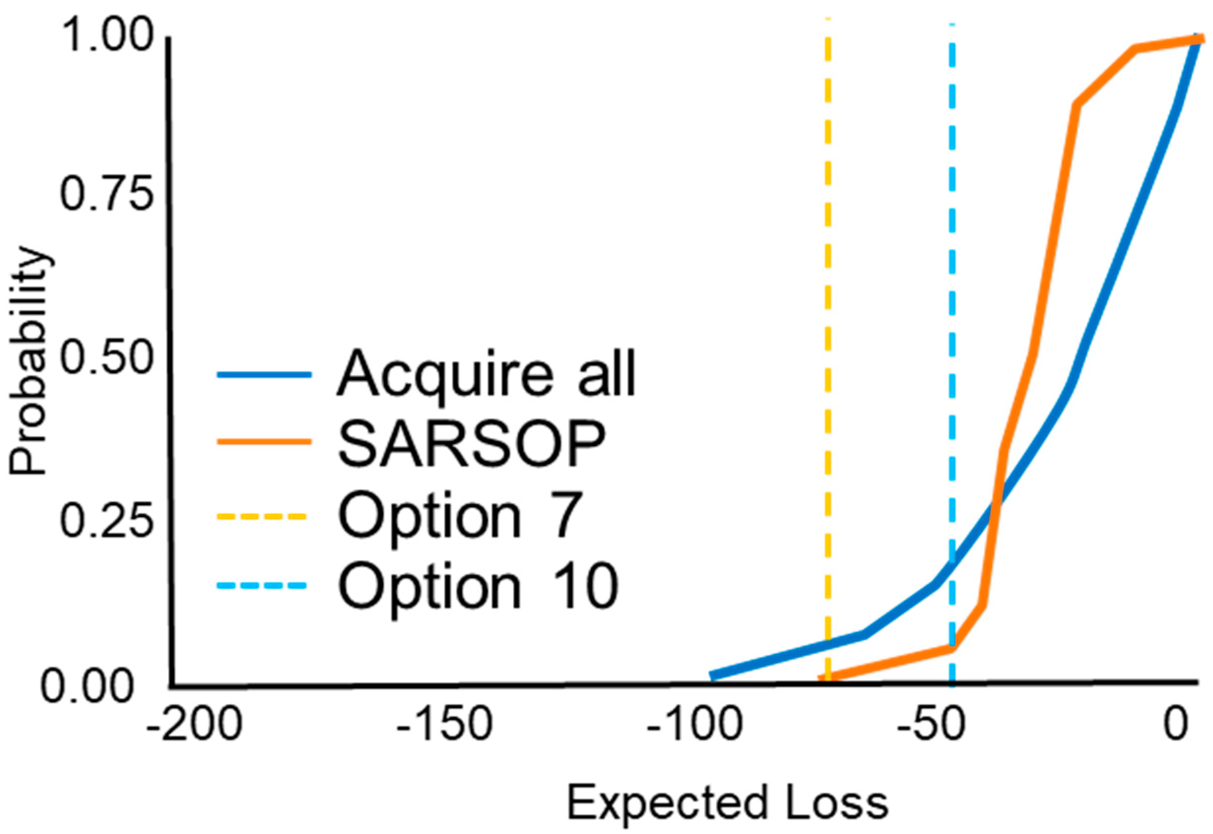
4.9.2. Results of the POMDP Agent
4.10. Human Suggested Data Acquisitions Strategies
4.11. Discussion of the Results of AI-Centric Evaluation Phase
5. Conclusions and Recommendations
Author Contributions
Funding
Data Availability Statement
Acknowledgments
Conflicts of Interest
Acronyms and Abbreviations
| AI | artificial intelligence |
| CAPEX | capital expenditures |
| CDF | cumulative distribution function |
| EMV | expected monetary value |
| FDP | field development plan |
| FID | final investment decision |
| KPI | key performance indicator |
| LHS | Latin hypercube sampling |
| NPV | net present value |
| OPEX | operating expenditures |
| P10, P50, P90 | 10%, 50%, 90% percentile |
| PES | probability of economic success |
| POM | probability of maturation |
| POMDP | partially observable Markov decision process |
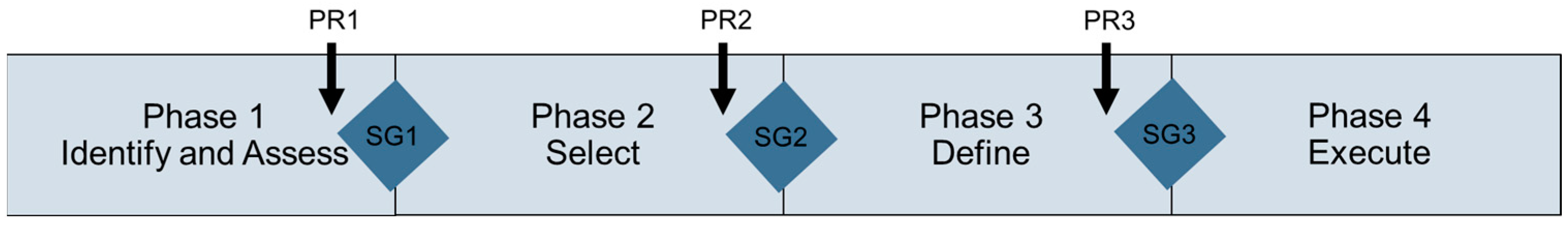
| PR | project review |
| VOI | value of information |
Appendix A


| Name | Minimum | Maximum | Unit |
|---|---|---|---|
| Porosity standard deviation | 0.01 | 0.02 | fraction |
| Porosity mean of the normal distribution | 0.065 | 0.135 | fraction |
| Azimuth of the variogram | 0 | 359 | degree |
| Variogram anisotropy—major direction | 200 | 5000 | m |
| Variogram anisotropy—minor direction | 200 | 1000 | m |
| Variogram anisotropy range—vertical direction | 10 | 100 | m |
| Fault transmissibility multiplier | 0 | 1 | - |
| Permeability ratio vertical/horizontal | 0.01 | 0.5 | - |
| Surface trend Z value maximum | 0.085 | 0.195 | - |
| Surface trend Z value minimum | 0.045 | 0.085 | - |
| Name | Minimum | Maximum | Unit |
|---|---|---|---|
| Water compressibility | 4.70 × 10⁻⁵ | 4.80 × 10⁻⁵ | 1/bar |
| Initial reservoir pressure | 240 | 250 | bar |
| Rock compressibility | 3.0 × 10⁻⁵ | 8.0 × 10⁻⁵ | 1/bar |
| Rock thermal conductivity | 238.7 | 292 | KJ/(mx dx K) |
| Rock heat capacity | 2303.5 | 3116.5 | KJ/(m3x K) |
| Temperature gradient | 0.025 | 0.035 |
| Name | Minimum | Maximum | Unit |
|---|---|---|---|
| Energy (heat) price | 1.1 10−5 | 1.67 10−5 | EUR/kJ |
| CAPEX injection well | 4 | 8 | EUR M |
| CAPEX production well | 4 | 8 | EUR M |
| CAPEX surface facilities | See Table A4 | See Table A4 | |
| CAPEX flowlines | See Table A4 | See Table A4 | |
| CAPEX production pump | 0.25 | 0.4 | EUR M |
| CAPEX injection pump | 0.15 | 0.25 | EUR M |
| OPEX fixed total | See Table A4 | See Table A4 | |
| OPEX surface facilities | 4.5 | 6 | % of Surface Facility CAPEX |
| OPEX water | 0.17 | 0.22 | EUR/(m3 year) |
| OPEX water injectors | 0.17 | 0.22 | EUR/(m3 year) |
| OPEX active producers | 0.09 | 0.15 | EUR/(well year) |
| OPEX active water injectors | 0.09 | 0.15 | EUR/(well year) |
| Option Number | Facility Type | CAPEX Surface Facilities | CAPEX Flowlines | OPEX Fixed Total |
|---|---|---|---|---|
| 1 | Large | EUR 300–500 M | EUR 100–140 M | EUR 27–39 M |
| 2 | Large | EUR 300–500 M | EUR 100–140 M | EUR 29–42 M |
| 3 | Large | EUR 300–500 M | EUR 100–140 M | EUR 26–38 M |
| 4 | Large | EUR 300–500 M | EUR 100–140 M | EUR 27–39 M |
| 5 | Medium | EUR 270–450 M | EUR 90–126 M | EUR 20–29 M |
| 6 | Medium | EUR 270–450 M | EUR 90–126 M | EUR 17–25 M |
| 7 | Small | EUR 255–425 M | EUR 85–119 M | EUR 12–18 M |
| 8 | Small | EUR 255–425 M | EUR 79–105 M | EUR 8–12 M |
| 9 | Medium | EUR 270–450 M | EUR 90–126 M | EUR 20–29 M |
| 10 | Medium | EUR 270–450 M | EUR 90–126 M | EUR 20–29 M |
| 11 | Medium | EUR 270–450 M | EUR 90–126 M | EUR 19–28 M |
| Human Expert Policy | EMV in EUR M | Number of Acquisition Actions | Data Acquisitions Costs in EUR M |
|---|---|---|---|
| 1 | 75 | 16 | −34 |
| 2 | 76 | 6 | −25 |
| 3 | 92 | 3 | −12 |
| 4 | 84 | 9 | −25 |
| 5 | 99 | 8 | −14 |
| 6 | 107 | 5 | −2 |
| 7 | 71 | 13 | −37 |
| 8 | 71 | 10 | −37 |
| 9 | 68 | 8 | −37 |
References
- IRENA; IGA. Global Geothermal Market and Technology Assessment; International Renewable Energy Agency: Abu Dhabi, United Arab Emirates; International Geothermal Association: The Hague, The Netherlands, 2023. [Google Scholar]
- Fraunhofer IWES/IBP (2017): Wärmewende 2030. Schlüsseltechnologien zur Erreichung der Mittel und Langfristigen Klimaschutzziele im Gebäudesektor. Studie im Auftrag von Agora Energiewende. Agora Energiewende, Berlin, Germany; Studie 107/01-S-2017/DE. Available online: https://www.agora-energiewende.de/ (accessed on 10 January 2024).
- Acksel, D.; Amann, F.; Bremer, J.; Bruhn, D.; Budt, M.; Bussmann, G.; Görke, J.-U.; Grün, G.; Hahn, F.; Hanßke, A.; et al. Roadmap Tiefe Geothermie für Deutschland—Handlungsempfehlungen für Politik, Wirtschaft und Wissenschaft für Eine Erfolgreiche Wärmewende. Strategiepapier von sechs Einrichtungen der Frauenhofer Gesellschaft und der Helmholtz-Gemeinschaft; Fraunhofer Einrichtung für Energieinfrastrukturen und Geothermie, Achen, Germany Helmholtz-Zentrum Potsdam Deutsches GeoForschungsZentrum: Potsdam, Germany, 2022. [Google Scholar] [CrossRef]
- Baumann, M.; Pauritsch, G.; Rohre, M. Roadmap zur Dekarbonisierung der Fernwärme in Österreich; Endbericht Austrian Energy Agency: Wien, Austria, 2020. [Google Scholar]
- BMK. FTI-Roadmap Geothermie—Vision und FTI-Politische Fragestellungen; Bericht, BMK Bundesministerium für Klimaschutz, Umwelt, Energie, Mobilität, Innovation und Technologie: Wien, Austria, 2022. [Google Scholar]
- Ciucci, M. Innovative Technologies in the Development of Geothermal Energy in Europe; Briefing Requested by the ITRE Committee; PE754.200; European Parliament: Luxembourg, 2023. [Google Scholar]
- Poulsen, S.E.; Balling, N.; Nielsen, S.B. A parametric study of the thermal recharge of low enthalpy geothermal reservoirs. Geothermics 2015, 53, 464–478. [Google Scholar] [CrossRef]
- Crooijmans, R.A.; Willems, C.J.L.; Nick, H.M.; Bruhn, D.F. The influence of facies heterogeneity on the doublet performance in low-enthalpy geothermal sedimentary reservoirs. Geothermics 2016, 64, 209–219. [Google Scholar] [CrossRef]
- Shetty, S.; Voskov, D.; Bruhn, D. Numerical Strategy for Uncertainty Quantification in Low Enthalpy Geothermal Projects. In Proceedings of the 43rd Workshop on Geothermal Reservoir Engineering Stanford University, Stanford, CA, USA, 12–14 February 2018. Paper SGP-TR-213. [Google Scholar]
- Ganguly, S.; Tan, L.; Date, A.; Kumar, M. Numerical investigation of temperature distribution in a confined heterogeneous geothermal reservoir due to injection-production. Energy Procedia 2017, 110, 143–148. [Google Scholar] [CrossRef]
- Rioseco, E.M.; Ziesch, J.; Wawerzinek, B.; Von Hartmann, H.; Thomas, R.; Buness, H. 3-D Geothermal Reservoir Modeling of the Upper Jurassic Carbonate Aquifer in the City of Munich (Germany) under the Thermal-Hydraulic Influence of Optimized Geothermal Multi-Well Patterns—Project GeoParaMoL. In Proceedings of the 43rd Workshop on Geothermal Reservoir Engineering Stanford University, Stanford, CA, USA, 12–14 February 2018. Paper SGP-TR-213. [Google Scholar]
- Babaei, M.; Nick, H.M. Performance of low-enthalpy geothermal systems: Interplay of spatially correlated heterogeneity and well-doublet spacings. Appl. Energy 2019, 253, 113569. [Google Scholar] [CrossRef]
- Willems, C.J.L.; Nick, H.M. Towards optimization of geothermal heat recovery: An example from the West Netherlands Basin. Appl. Energy 2019, 247, 582–593. [Google Scholar] [CrossRef]
- Bayerl, M.; Ebner, M.; Clemens, T. Forecasting Low Enthalpy Geothermal Heat Extraction from Saline Aquifers Under Uncertainty. In Proceedings of the SPE Europe Energy Conference Featured at the 84th EAGE Annual Conference and Exhibition, Vienna, Austria, 5–8 June 2023. Paper SPE-214413. [Google Scholar]
- Schulte, D.O.; Arnold, D.; Geiger, S.; Demyanov, V.; Sass, I. Multi-objective optimization under uncertainty of geothermal reservoirs using experimental design-based proxy models. Geothermics 2020, 86, 101792. [Google Scholar] [CrossRef]
- Juliusson, E.; Bjornsson, S. Optimizing production strategies for geothermal resources. Geothermics 2021, 94, 102091. [Google Scholar] [CrossRef]
- Trainor-Guitton, W.J.; Hoversten, G.M.; Nordquist, G.; Intani, R.G. Value of Information Analysis Using Geothermal Field Data: Accounting for Multiple Interpretations & Determining New Drilling Locations; SEG Technical Program Expanded Abstracts; Society of Exploration Geophysicists: Houston, TX, USA, 2015. [Google Scholar]
- Porlles, J.W.; Jabbari, H. Simulation-Based Patterns Optimization of Enhanced Geothermal Systems. In Proceedings of the 56th US Rock Mechanics/Geomechanics Symposium, Santa Fe, CA, USA, 26–29 June 2022. Paper ARMA 22-2321. [Google Scholar]
- Williams, C.F. Development of Revised Techniques for Assessing Geothermal Resources. In Proceedings of the Twenty-Ninth Workshop on Geothermal Reservoir Engineering Stanford University, Stanford, CA, USA, 26–28 January 2004. Paper SGP-TR-175. [Google Scholar]
- Falcone, G.; Gnoni, A.; Harrison, B.; Alimonti, C. Classification and Reporting Requirements for Geothermal Resources. In Proceedings of the European Geothermal Congress, Pisa, Italy, 3–7 June 2013. [Google Scholar]
- Dewi, M.P.; Setiawan, A.D.; Latief, Y.; Purwanto, W.W. Investment decisions under uncertainties in geothermal power generation. AIMS Energy 2022, 10, 844–857. [Google Scholar] [CrossRef]
- Nandurdikar, N.; Wallace, L. Failure to Produce: An Investigation of Deficiencies in Production Attainment. In Proceedings of the SPE Annual Technical Conference and Exhibition, Denver, CO, USA, 30 October–2 November 2011. Paper SPE 145437. [Google Scholar]
- Nesvold, E.; Bratvold, R.B. Field Features Do Not Explain Greenfield Production Forecasting Bias. SPE J. 2022, 28, 1290–1307. [Google Scholar] [CrossRef]
- Wang, L.; Oliver, D.S. Efficient Optimization of Well-Drilling Sequence with Learned Heuristics. SPE J. 2019, 24, 2111–2134. [Google Scholar] [CrossRef]
- Bailey, W.; Prange, M. Flow Control Valve Valuation and Value of Information under Uncertainty. SPE J. 2023, 28, 2036–2051. [Google Scholar] [CrossRef]
- Steineder, D.; Clemens, T. Hydrocarbon Field Re-Development in a Bayesian Framework. In Proceedings of the SPE Europec Featured at 82nd EAGE Conference and Exhibition, Amsterdam, The Netherlands, 18–21 October 2021. Paper SPE 205227. [Google Scholar]
- Soltani, M.; Kashkooli, F.M.; Souri, M.; Rafiei, B.; Jabarifar, M.; Gharali, K.; Nathwani, J.S. Envirnomental, economic and social impacts of geothermal energy systems. Renew. Sustain. Energy 2021, 140, 110750. [Google Scholar] [CrossRef]
- Russel, S.; Norvig, P. Artificial Intelligence: A Modern Approach, 4th ed.; Pearson: London, UK, 2021. [Google Scholar]
- Kochenderfer, M.J. Decision Making Under Uncertainty: Theory and Application; MIT Press: Cambridge, MA, USA, 2015. [Google Scholar]
- Ayer, O.A.; Stout, N.K. A POMDP Approach to Personalize Mammography Screening Decisions. Oper. Res. 2012, 60, 1019–1034. [Google Scholar] [CrossRef]
- Wang, Y.; Dong, W.; Yang, Q. Multi-stage optimal energy management of multi-energy microgrid in deregulated electricity markets. Appl. Energy 2022, 310, 118528. [Google Scholar] [CrossRef]
- De Paola, G.; Ibanez-Llano, C.; Rios, J.; Kollias, G. Reinforcement Learning for Field Development Policy Optimization. In Proceedings of the SPE Annual Technical Conference & Exhibition, Denver, CO, USA, 5–7 October 2020. Paper SPE 201254. [Google Scholar]
- He, J.; Tang, M.; Hu, C.; Tanaka, S.; Wang, K.; Wen, X.-H.; Nasir, Y. Deep Reinforcement Learning for Generalizable Field Development Optimization. SPE J. 2021, 27, 226–245. [Google Scholar] [CrossRef]
- Gehringer, M.; Loksha, V. Geothermal Handbook: Planning and Financing Power Generation; ESMAP Technical Report 002/12; The International Bank for Reconstruction and Development: Washington, DC, USA, 2012. [Google Scholar]
- IGA. Best Practices Guide for Geothermal Exploration; Report IGA Service GmbH; IGA: Bochum, Germany, 2014. [Google Scholar]
- Gudmundsson, Y. Geothermal Project Timelines. In Proceedings of the 6th African Rift Geothermal Conference, Addis Ababa, Ethiopia, 2–4 November 2016. [Google Scholar]
- Walkup, G.W.; Ligon, J.R. The Good, the Bad, and the Ugly of the Stage-Gate Project Management Process in the Oil and Gas Industry. In Proceedings of the 2006 SPE Annual Technical Conference and Exhibition, San Antonio, TX, USA, 24–27 September 2006. Paper SPE 102926. [Google Scholar]
- Merrow, E.W. Oil and Gas Industry Megaprojects: Our Recent Track Record. Oil Gas Facil. 2012, 1, 38–42. [Google Scholar] [CrossRef]
- Bratvold, R.B.; Bickel, J.E.; Lohne, H.P. Value of Information in the Oil and Gas Industry: Past, Present, and Future. SPE Reserv. Eval. Eng. 2009, 12, 630–6384. [Google Scholar] [CrossRef]
- Aragon, A.; Izquiedo-Montalvo, G.; Aragon-Gaspar, D.O.; Barreto-Rivera, D.N. Stages of as Integrated Geothermal Project. In Book Renewable Geothermal Energy Explorations; IntechOpen: London, UK, 2019. [Google Scholar] [CrossRef]
- Cooper, R.G. Stage-gate systems: A new tool for managing new products. Bus. Horizons 1990, 33, 44–54. [Google Scholar] [CrossRef]
- Mishar, S.N. Improving Major Project Development through a Front End Loading Management System: Medco’s way for Oil & Gas Development Project. In Proceedings of the SPE 162254 presented at the Abu Dhabi International Petroleum Exhibition & Conference, Abu Dhabi, United Arab Emirates, 11–14 November 2012. [Google Scholar]
- Ambrose, J.; Monette, S.A.; Malani, S. Make Better Decisions. In Proceedings of the SPE Hydrocarbon Economics and Evaluation Symposium, Houston, TX, USA, 19–20 May 2014. SPE Paper 169846. [Google Scholar]
- Khalil, T.; Balsubramanian, N.; Lugon, P. ADNOC Journey in Developing an Unified Value Assurance Process for Capital Investment Projects. In Proceedings of the Abu Dhabi International Petroleum Exhibition & Conference, Abu Dhabi, United Arab Emirates, 13–16 November 2017. Paper SPE 188485. [Google Scholar]
- Safra, E.B.; Antelo, S.B. Integrated Project Management Applied in World-Class Gas-Field Development Projects: From Theory to Practice. In Proceedings of the SPE Latin American & Caribbean Petroleum Engineering Conference, Lima, Peru, 1–3 December 2010. Paper SPE 139369. [Google Scholar]
- Gao, G.; Lu, H.; Wang, K.; Jost, S.; Shaikh, S.; Vink, J.; Blom, C.; Wells, T.; Saaf, F. A Practical Approach to Select Representative Deterministic Models Using Multiobjective Optimization from an Integrated Uncertainty Workstream. SPE J. 2023, 28, 2186–2206. [Google Scholar] [CrossRef]
- Balasubramanian, S.; Wang, B.; Li, Y.; Ginger, E.P.; Liang, B.; McKay, D.M.; Brinkman, J.J.; Ogden, K.A.; Kennedy, D.D.; Wilcox, W.T.; et al. Subsurface Appraisal and Field Development Planning of the Gas Condensate Field GVLA. In Proceedings of the Offshore Technology Conference, Houston, TX, USA, 6–9 May 2013. Paper OTC 24108. [Google Scholar]
- Alkhatib, M.; Ali, A.A.A.; Mukhtar, M.; Park, S.; Ghorayeb, K.; Nasiri, A.; Sha, A.R.; Ojha, A. A Novel Holistic Workflow for Field Development Planning in Green Field Envirnoment: A Case Study. In Proceedings of the Abu Dhabi International Petroleum Exhibition & Conference, Abu Dhabi, United Arab Emirates, 12–15 November 2018. Paper SPE 193140. [Google Scholar]
- Ibrahimov, T. History of History Match in Azeri Field. In Proceedings of the SPE Annual Caspian Technical Conference & Exhibition, Baku, Azerbaijan, 4–6 November 2015. Paper SPE 177395. [Google Scholar]
- Spetzler, C.; Winter, H.; Meyer, J. Decision Quality: Value Creation from Better Business Decisions; Wiley: Hoboken, NJ, USA, 2016. [Google Scholar]
- Sauve, R.; Lindvig, T.; Stenhaug, M.; Holyfield, S. Integrated Field Development: Process and Productivity. In Proceedings of the Offshore Technology Conference, Houston, TX, USA, 6–9 May 2019. Paper OTC-29631. [Google Scholar]
- Siler, D.L.; Pepin, J.D.; Vessilinov, V.V.; Mudunuru, M.K.; Ahmmed, B. Machine learning to identify geological factors associated with production in geothermal fields: A case-study using 3D geologic data, Brady geothermal field, Nevada. Geotherm. Energy 2021, 9, 17. [Google Scholar] [CrossRef]
- Suzuki, A.; Fukui, K.-I.; Onodera, S.; Ishizaki, J.; Hashida, T. Data-Driven Geothermal Reservoir Modeling: Estimating Permeability Distributions by Machine Learning. Geosciences 2022, 12, 130. [Google Scholar] [CrossRef]
- Major, M.; Daniilidis, A.; Hansen, T.M.; Khait, M.; Voskov, D. Influence of process-based, stochastic and deterministic methods for representing heterogeneity in fluvial geothermal systems. Geothermics 2023, 109, 102651. [Google Scholar] [CrossRef]
- Kochenderfer, M.J.; Tim, A.; Wheeler, T.A.; Wray, K.A. Algorithms for Decision Making; MIT Press: Cambridge, MA, USA, 2022. [Google Scholar]
- Tversky, A.; Kahneman, D. Judgment under Uncertainty: Heuristics and Biases. Science 1974, 185, 1124–1131. [Google Scholar] [CrossRef] [PubMed]
- Choi, S.; Kim, N.; Kim, J.; Kang, H. How Does AI Improve Human Decision-Making? Evidence from the AI-Powered Go Program. USC Marshall School of Business Research Paper Sponsored by iORB, No. Forthcoming. 2023. Available online: https://ssrn.com/abstract=3893835 (accessed on 14 January 2024).
- SPE. Guidance for Decision Quality for Multicompany Upstream Projects; Technical Report SPE 181246; Society of Petroleum Engineers: Dallas, TX, USA, 2016. [Google Scholar]
- Schuyler, J. Portfolio Management: What is the Contribution to Shareholder Value? In Proceedings of the SPE Hydrocarbon Economics and Evaluation Symposium, Dallas, TX, USA, 5–8 April 2003. Paper SPE 82031. [Google Scholar]
- Holden, C.W. Maximizing Portfolio Value with Specified Assurance. In Proceedings of the 2005 SPE Hydrocarbon Economics and Evaluation Symposium, Dallas, TX, USA, 3–5 April 2005. Paper SPE 94438. [Google Scholar]
- Allen, D.P.B. Handling Risk and Uncertainty in Portfolio Production Forecasting. SPE Econ. Manag. 2017, 9, 37–42. [Google Scholar] [CrossRef]
- Luan, P. How To Avoid Project Train Wrecks. Oil Gas Facil. 2016, 5, 24–28. [Google Scholar] [CrossRef]
- Paribelli, L.; Guarino, M. Project Strategic Framing Approach—The Strategy Table. In Proceedings of the Abu Dhabi International Petroleum Exhibition and Conference, Abu Dhabi, United Arab Emirates, 15–18 November 2021. Paper SPE 207323. [Google Scholar]
- Harzhauser, M.; Kranner, M.; Mandic, O.; Strauss, P.; Siedl, W.; Piller, W.E. Miocene lithostratigraphy of the northern and central Vienna Basin (Austria). Austrian J. Earth Sci. 2020, 113, 169–199. [Google Scholar] [CrossRef]
- Büchele, R.; Haas, R.; Hartner, M.; Hirner, R.; Hummel, M.; Kranzl, L.; Müller, A.; Ponweiser, K.; Bons, M.; Grave, K.; et al. Bewertung des Potenzials für den Hocheffizienten KWK und Effizienter Fernwärme- und Fernkälteversorgung; Technical Report TU Wien and Ecofys; Technical UniversityWien and Ecofys: Wien, Austria, 2015. [Google Scholar]
- Königshofer, K.; Domberger, G.; Gunczy, S.; Hingsamer, M.; Pucker, J.; Schreilechner, M.; Amtmann, J.; Goldbrunner, J.; Heiss, H.P.; Füreder, J.; et al. Potenzial der Tiefengeothermie für die Fernwärme- und Stromproduktion in Österreich; Joanneum Research Forschungsgesellschaft mbH: Graz, Austria, 2014. [Google Scholar]
- Wessely, G. Structure and development of the Vienna basin in Austria. Am. Assoc. Petrol. Geol. Mem. 1988, 45, 333–346. [Google Scholar]
- Arzmüller, G.; Buchta, S.B.; Ralbovsky, E.; Wessely, G. The Vienna Basin. In The Carpathians and Their Foreland: Geology and Hydrocarbon Resources, AAPG Memoir 84; Golonka, J., Picha, F.J., Eds.; American Association of Petroleum Geologists: Tulsa, OK, USA, 2006; pp. 191–204. [Google Scholar] [CrossRef]
- Weissenbäck, M. Lower to Middle Miocene sedimentation model of the central Vienna Basin. In Oil and Gas in Alpidic Thrustbelts and Basins of Central and Eastern Europe; Special Publications 5; European Association of Geoscientists and Engineers EAGE: Utrecht, The Netherlands, 1996; pp. 355–363. [Google Scholar]
- Corso, A.; Chiotoroiu, M.; Clemens, T.; Zechner, M.; Kochenderfer, M.J. Sequentially optimized data acquisition for a geothermal reservoir. Geothermics 2024, 120, 102983. [Google Scholar] [CrossRef]
- Sieberer, M.; Clemens, T.; Peisker, J.; Ofori, S. Polymer-Flood Field Implementation: Pattern Configuration and Horizontal vs. Vertical Wells. SPE Reserv. Eval. Eng. 2019, 22, 577–596. [Google Scholar] [CrossRef]
- Blank, L.; Rioseco, E.M.; Caiazzo, A.; Wilbrandt, U. Modeling, simulation, and optimization of geothermal energy production from hot sedimentary aquifers. Comput. Geosci. 2020, 25, 67–104. [Google Scholar] [CrossRef]
- Steineder, D.; Clemens, T. Including Oil Price Uncertainty in Development Option Selection Taking the Project Portfolio into Account. In Proceedings of the SPE Europec Featured at 81st EAGE Conference and Exhibition, London, UK, 3–6 June 2019. Paper SPE 195440. [Google Scholar]
- Narayanan, M.; Abdulazeez, M.; Bukhamsin, K.; Alshehri, N. Stochastic Economic Ranking—A Prudent Way to Address Risk and Uncertainty for Decision Makers. In Proceedings of the Middle East Oil, Gas and Geosciences Show, Manama, Bahrain, 19–21 February 2023. Paper SPE 213385. [Google Scholar]
- Demirmen, F. Use of “Value of Information” Concept in Justification and Ranking of Subsurface Appraisal. In Proceedings of the SPE Annual Technical Conference and Exhibition, Denver, CO, USA, 6–9 October 1996. Paper SPE 36631. [Google Scholar]
- Bratvold, R.B.; Mohus, E.; Petutschnig, D.; Bickel, E. Production Forecasting: Optimistic and Overconfident—Over and Over Again. SPE Reserv. Eval. Eng. 2020, 23, 0799–0810. [Google Scholar] [CrossRef]
- Fenwick, D.; Scheidt, C.; Caers, J. Quantifying Asymmetric Parameter Interactions in Sensitivity Analysis: Application to Reservoir Modeling. Math. Geosci. 2014, 46, 493–511. [Google Scholar] [CrossRef]
- Kurniawati, H.; Hsu, D.; Lee, W.S. SARSOP: Efficient point-based POMDP planning by approximating optimally reachable belief spaces. In Robotics: Science and Systems; MIT Press: Cambridge, MA, USA, 2008. [Google Scholar]
- Leeftink, T.; Velez, D.A.; Godderij, R. Overestimation in Operators Budgets and Long-Term Forecasting; A Non-Operator Perspective. In Proceedings of the SPE Europec featured at the 81st EAGE Conference and Exhibition, London, UK, 23–26 June 2019. Paper SPE 195519. [Google Scholar]
- Van der Haar, K. The Contingent Resources Class: Non-Differentiation of Contingent Resources and Its Implications. In Proceedings of the SPE/IATMI Asia Pacific Oil and Gas Conference and Exhibition, Jakarta, Indonesia, 10–12 October 2023. Paper SPE 215462. [Google Scholar]
- Koninx, J.P.M. Value of Information: From Cost Cutting to Value Creation. J. Pet. Technol. 2001, 53, SPE 69836. [Google Scholar] [CrossRef]
- Coopersmith, E.M.; Cunningham, P.C. A Practical Approach to Evaluating the Value of Information and Real Option Decisions in the Upstream Petroleum Industry. In Proceedings of the SPE Annual Technical Conference and Exhibition, San Antonio, TX, USA, 29 September–2 October 2002. Paper SPE 77582. [Google Scholar]
- Wills, H.A.; Graves, R.M.; Miskimins, J. Don’t Be Fooled by Bayes. In Proceedings of the SPE Annual Technical Conference and Exhibition, Houston, TX, USA, 26–29 September 2004. Paper SPE 90717. [Google Scholar]
- Santos, S.M.G.; Schiozer, D.J. Assessing the Value of Information According to Attitudes Towards Downside Risk and Upside Potential. In Proceedings of the SPE Europec Featured at 79th EAGE Annual Conference and Exhibition, Paris, France, 12–15 June 2017. Paper SPE 185841. [Google Scholar]
- Steineder, D.; Clemens, T.; Osivandi, K.; Thiele, M.R. Maximizing the Value of Information of a Horizontal Polymer Pilot Under Uncertainty Incorporating the Risk Attitude of the Decision Maker. SPE Reserv. Eval. Eng. 2018, 22, 756–774. [Google Scholar] [CrossRef]
- El Souki, O.A.; Saad, G.A. A Stochastic Approach for Optimal Sequencing of Appraisal Wells. SPE Reserv. Eval. Eng. 2016, 20, 334–341. [Google Scholar] [CrossRef]
- Trainor-Guitton, W. The value of geophysical data for geothermal exploration: Examples from empirical, field, and synthetic data. Geophysics 2020, 39, 864–872. [Google Scholar] [CrossRef]
- Akar, S.; Young, K.R. Assessment of New Approaches in Geothermal Exploration Decision Making. In Proceedings of the 40th Workshop on Geothermal Reservoir Engineering, Sanford, FL, USA, 26–28 January 2015. [Google Scholar]
- Bang, D.; Frith, C.D. Making better decisions in groups. R. Soc. Open Sci. 2017, 4, 170193. [Google Scholar] [CrossRef]
- Felfernig, A.; Müslum, A.; Martin Stettinger, M.; Tran, T.N.T.; Leitner, G. Biases in Group Decisions. In Group Recommender Systems—An Introduction; Felfernig, A., Boratto, L., Stettinger, M., Tkalcic, M., Eds.; Springer: Cham, Switzerland, 2018. [Google Scholar]


| Scenario Number | Facility Type | Pattern Type | Well Spacing in m | Number of Injectors | Number of Producers |
|---|---|---|---|---|---|
| 1 | Large | 5-spot | 400 | 39 | 39 |
| 2 | Large | LD EW | 400 | 37 | 42 |
| 3 | Large | LD NS | 400 | 41 | 38 |
| 4 | Large | 5-spot | 400 | 39 | 39 |
| 5 | Medium | 5-spot | 450 | 29 | 29 |
| 6 | Medium | 5-spot | 500 | 25 | 25 |
| 7 | Small | 5-spot | 600 | 18 | 18 |
| 8 | Small | 5-spot | 700 | 12 | 12 |
| 9 | Medium | LD EW | 450 | 29 | 29 |
| 10 | Medium | LD NS | 450 | 29 | 29 |
| 11 | Medium | LD EW | 465 | 28 | 28 |
| Option Number | EMV in EUR M | P10 NPV in EUR M | P50 NPV in EUR M | P90 NPV in EUR M | PES as Fraction |
|---|---|---|---|---|---|
| 1 | −86.74 | −488.28 | −102.89 | 344.09 | 0.38 |
| 2 | −40.48 | −466.64 | −57.73 | 417.19 | 0.44 |
| 3 | 3.81 | −437.88 | −12.75 | 472.34 | 0.49 |
| 4 | −111.85 | −604.72 | −105.14 | 367.17 | 0.38 |
| 5 | 28.42 | −333.13 | 15.58 | 411.85 | 0.52 |
| 6 | 81.63 | −279.84 | 74.21 | 460.50 | 0.60 |
| 7 | 105.98 | −201.51 | 106.19 | 423.01 | 0.65 |
| 8 | −6.21 | −236.42 | −6.24 | 233.66 | 0.49 |
| 9 | 59.04 | −324.04 | 48.01 | 464.37 | 0.56 |
| 10 | 105.07 | −294.11 | 95.85 | 524.52 | 0.62 |
| 11 | 95.80 | −291.37 | 85.10 | 504.01 | 0.61 |
| Name | Cost in EUR M | Duration in Years | Observed Variables | Observation Uncertainty |
|---|---|---|---|---|
| Water compressibility | −0.05 | 0.038 | Water compressibility | 5 × 10⁻⁵ 1/bar |
| Initial reservoir pressure | −0.01 | 0.058 | Initial reservoir pressure | 5 bar |
| Fault transmissibility multiplier | −2 | 0.16 | Fault transmissibility multiplier | 0.015 |
| Permeability ratio | −0.05 | 0.082 | Permeability ratio (vert/horiz) | 367.17 |
| Rock compressibility | −0.05 | 0.082 | Rock compressibility | 411.85 |
| Rock thermal conductivity | −0.05 | 0.082 | Rock thermal conductivity | 460.50 |
| Rock heat capacity | −0.05 | 0.082 | Rock heat capacity | 423.01 |
| Temperature gradient | −0.1 | 0.058 | Temperature gradient | 233.66 |
| Drill 3 wells | −9 | 0.74 | Porosity standard deviation Porosity mean Variogram anisotropy (major) Variogram anisotropy (minor) Variogram anisotropy (vertical) Variogram azimuth Surface trend Z max Surface trend Z min | 0.0025 0.025 1000 m 200 m 10 m 45 ° 0.045 0.015 |
| CAPEX injection well | −1.2 | 0.082 | CAPEX injection well | EUR 0.3 M |
| CAPEX production well | −1.2 | 0.082 | CAPEX production well | EUR 0.3 M |
| CAPEX surface facilities | −10 | 0.16 | CAPEX surface facilities | EUR 18 M |
| CAPEX flowlines | −10 | 0.16 | CAPEX flowlines | EUR 5.5 M |
| CAPEX production pump | −0.03 | 0.082 | CAPEX production pump | EUR 0.0162 M |
| CAPEX injection pump | −0.02 | 0.082 | CAPEX injection pump | EUR 0.01 M |
| OPEX fixed total | −3.5 | 0.082 | OPEX fixed total | 1.0 M EUR/year |
| OPEX water | −0.02 | 0.082 | OPEX water | 0.00975 EUR/m3/year |
| OPEX water injectors | −0.02 | 0.082 | OPEX water injectors | 0.00975 EUR/m3/year |
| OPEX active producers | −0.01 | 0.082 | OPEX active producers | 0.006 EUR/well/year |
| OPEX active water injectors | −0.01 | 0.082 | OPEX active water injectors | 0.006 EUR/well/year |
| Parameter | Value |
|---|---|
| epsilon | 0.5 |
| precision | 1 × 10⁻³ |
| kappa | 0.5 |
| delta | 1 × 10⁻¹ |
| max_time | 10 |
| max_steps | ∞ |
| init_lower | BlindLowerBound(bel_res = 1 × 10⁻²) |
| init_upper | FastInformedBound(bel_res = 1 × 10⁻²) |
| prunethresh | 0.1 |
| Policy | EMV in EUR M | Correct Go/No-Go | Correct Development Scenario | Number of Data Acquisition Actions | Expected Data Acquisition Costs in EUR M |
|---|---|---|---|---|---|
| Scenario 7 | 106 | 0.66 | 0.18 | 0 | 0 |
| Scenario 10 | 105 | 0.62 | 0.32 | 0 | 0 |
| Acquire all | 77 | 0.73 | 0.49 | 14.1 | 32 |
| SARSOP | 136 | 0.74 | 0.48 | 6.4 | 1.4 |
| Policy | EMV in EUR M | Correct Go/No-Go Decision | Correct Development Scenario | Data Acquisition Cost in EUR M |
|---|---|---|---|---|
| SARSOP | 136 | 0.737 | 0.476 | −1.4 |
| Best human (EMV, data acquisition): expert 6 | 107 | 0.66 | 0.32 | −2.2 |
| Best human (correct go/no-go and correct dev scen option): expert 1 | 75 | 0.728 | 0.5 | −33.8 |
| Average human | 83 | 0.67 | 0.38 | −24.7 |
Disclaimer/Publisher’s Note: The statements, opinions and data contained in all publications are solely those of the individual author(s) and contributor(s) and not of MDPI and/or the editor(s). MDPI and/or the editor(s) disclaim responsibility for any injury to people or property resulting from any ideas, methods, instructions or products referred to in the content. |
© 2024 by the authors. Licensee MDPI, Basel, Switzerland. This article is an open access article distributed under the terms and conditions of the Creative Commons Attribution (CC BY) license (https://creativecommons.org/licenses/by/4.0/).
Share and Cite
Clemens, T.; Chiotoroiu, M.-M.; Corso, A.; Zechner, M.; Kochenderfer, M.J. Artificial Intelligence-Centric Low-Enthalpy Geothermal Field Development Planning. Energies 2024, 17, 1887. https://doi.org/10.3390/en17081887
Clemens T, Chiotoroiu M-M, Corso A, Zechner M, Kochenderfer MJ. Artificial Intelligence-Centric Low-Enthalpy Geothermal Field Development Planning. Energies. 2024; 17(8):1887. https://doi.org/10.3390/en17081887
Chicago/Turabian StyleClemens, Torsten, Maria-Magdalena Chiotoroiu, Anthony Corso, Markus Zechner, and Mykel J. Kochenderfer. 2024. "Artificial Intelligence-Centric Low-Enthalpy Geothermal Field Development Planning" Energies 17, no. 8: 1887. https://doi.org/10.3390/en17081887
APA StyleClemens, T., Chiotoroiu, M.-M., Corso, A., Zechner, M., & Kochenderfer, M. J. (2024). Artificial Intelligence-Centric Low-Enthalpy Geothermal Field Development Planning. Energies, 17(8), 1887. https://doi.org/10.3390/en17081887