


Non-Iterative Coordinated Optimisation of Power–Traffic Networks Based on Equivalent Projection


Abstract
1. Introduction
2. Power–Traffic Coupled Model Equation
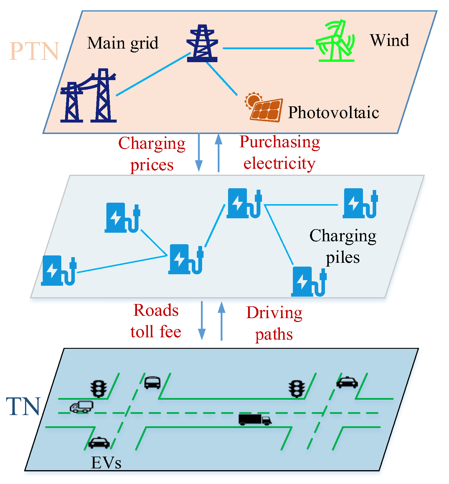
2.1. Interaction of the Coupled PTNs
2.2. A Traffic Model for the Travel Characteristics of Vehicles
2.2.1. Road Congestion Analysis Based on Various Types of EVs
- Charging links with EVCSs
- 2.
- Regular links without EVCSs
- 3.
- Bypass links
2.2.2. Modelling the Costs of Vehicles Based on Different Driving Behaviours
- The travel costs of EVs with charging
- 2.
- The travel costs of regular EVs
2.2.3. A Traffic Model Based on User Equilibrium
2.3. Modelling of the Optimal Power Flow in the PDN
2.4. Modelling of the Coupled PTN
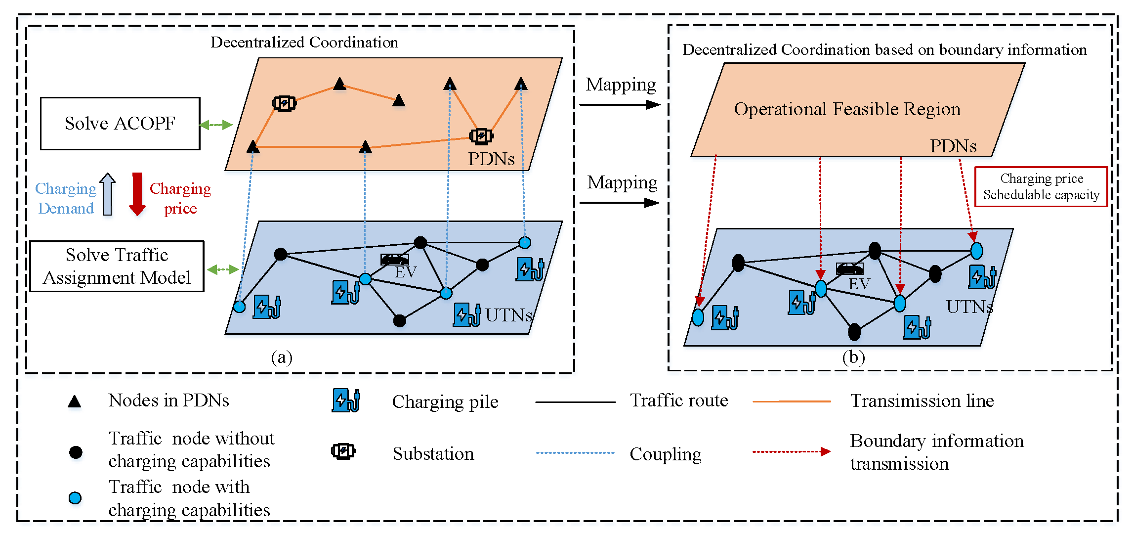
3. Decoupled Model of the PTN Based on the Feasible Region of the PDN
4. Mapping Optimal Costs of the PDNs
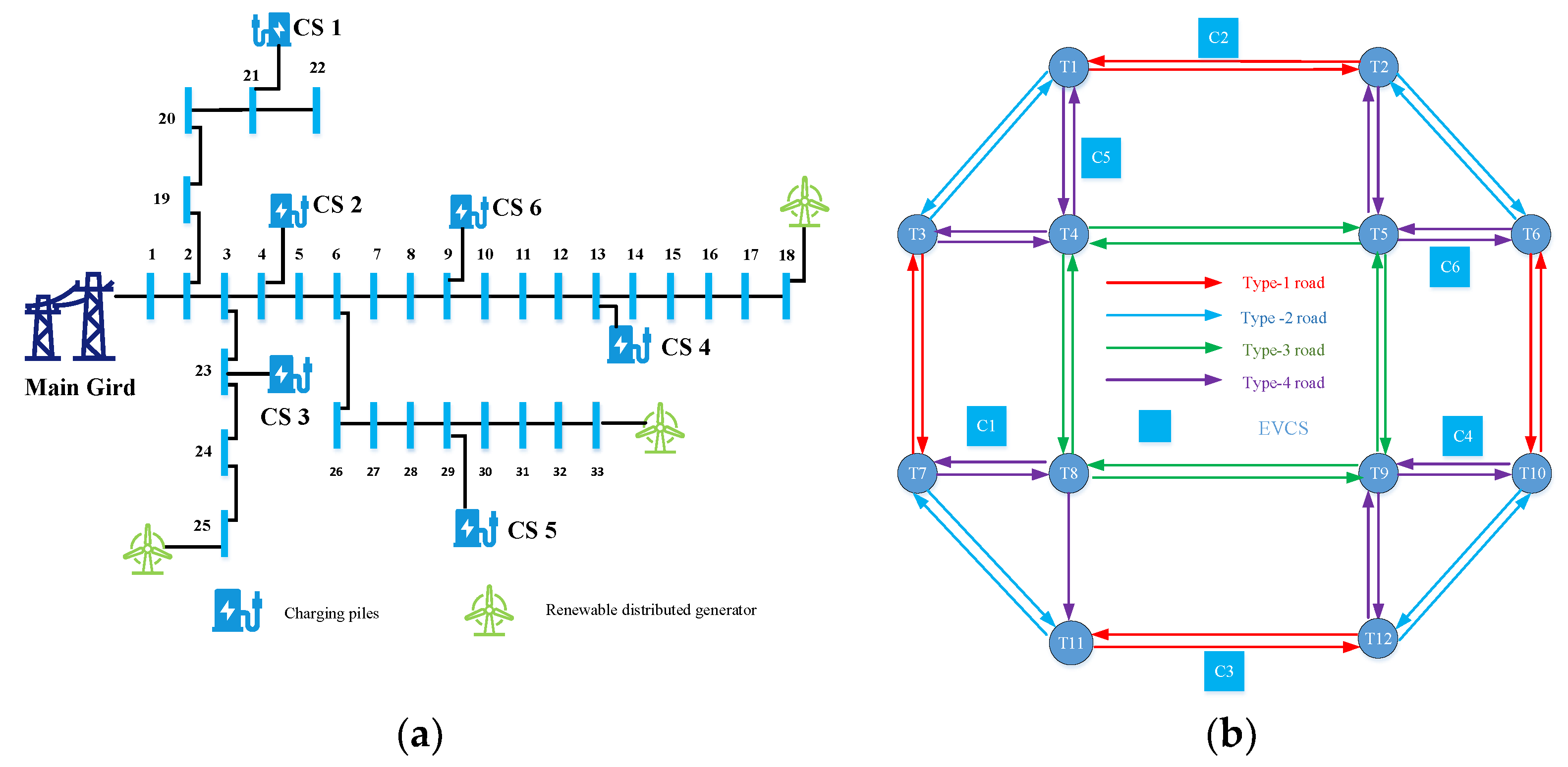
5. Case Study
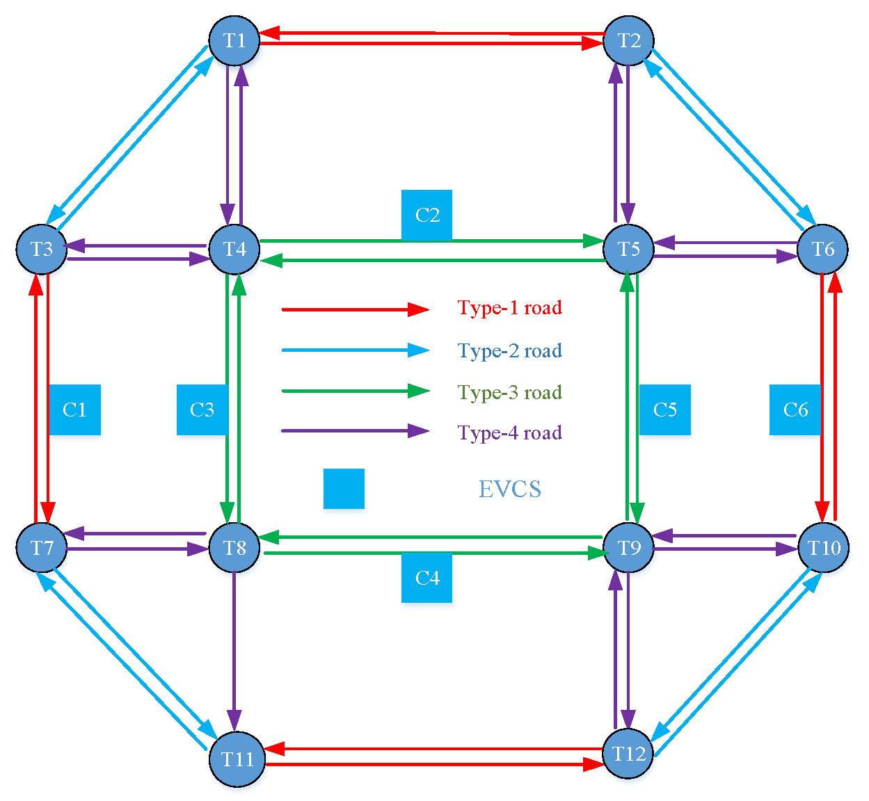
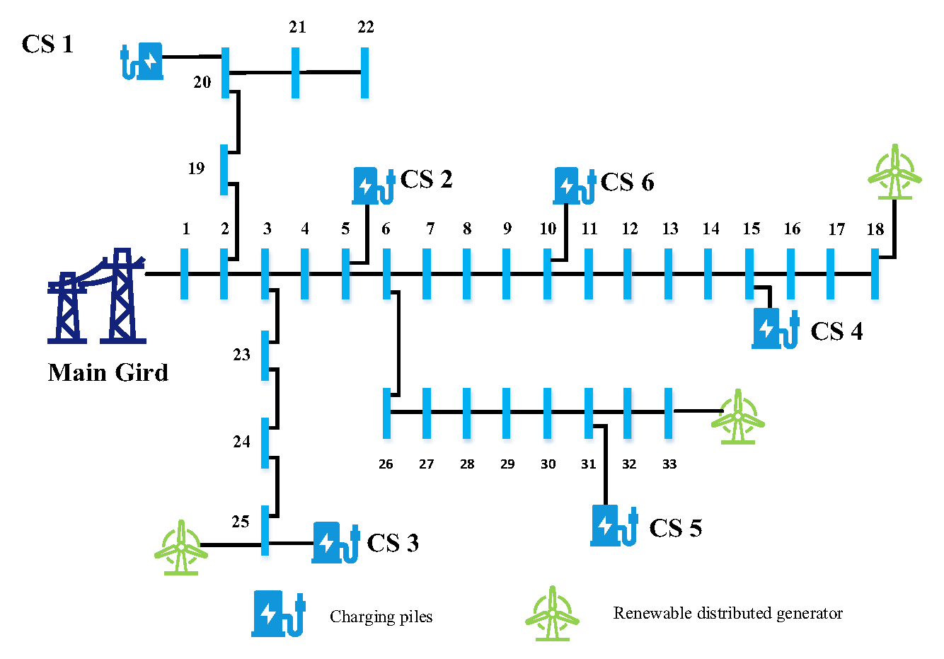
5.1. Basic Settings
5.2. Analysis Discussion
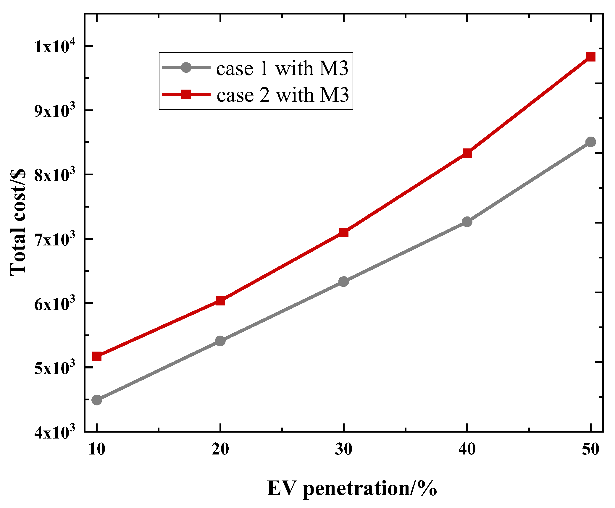
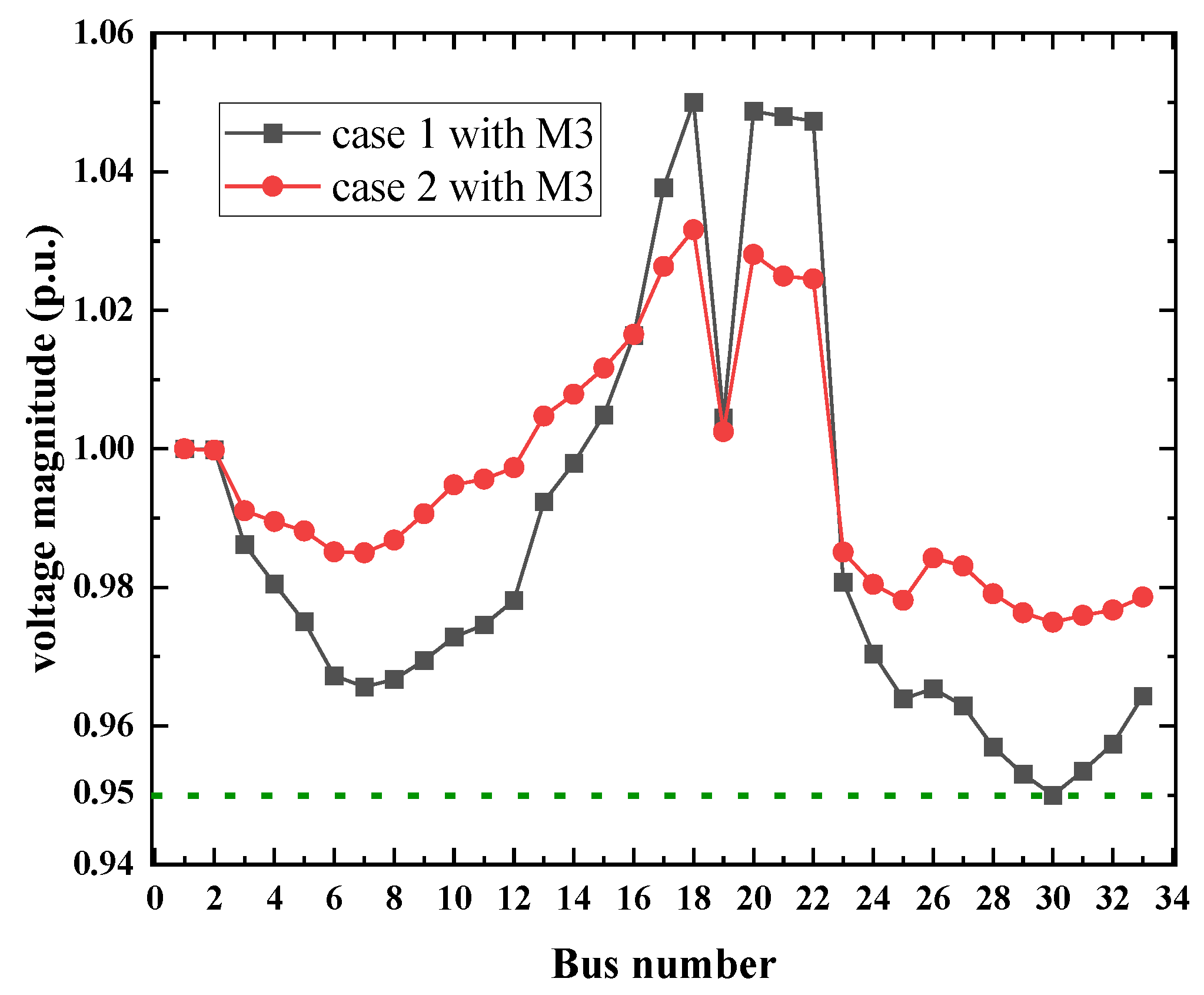
5.3. Comparative Analysis of the Case Studies
6. Conclusions
Author Contributions
Funding
Data Availability Statement
Acknowledgments
Conflicts of Interest
References
- Lopes, J.A.P.; Soares, F.J.; Almeida, P.M.R. Integration of Electric Vehicles in the Electric Power System. Proc. IEEE 2011, 99, 168–183. [Google Scholar] [CrossRef]
- Global EV Outlook 2022 [EB/OL]. [Online]. Available online: https://www.iea.org/reports/global-ev-outlook-2022 (accessed on 25 December 2023).
- Kezunovic, M.; Waller, S.T.; Damnjanovic, I. Framework for studying emerging policy issues associated with phevs in managing coupled power and transportation systems. In Proceedings of the 2010 IEEE Green Technologies Conference, Grapevine, TX, USA, 15–16 April 2010; pp. 1–8. [Google Scholar]
- Yang, W.; Liu, W.; Chung, C.Y.; Wen, F. Joint planning of EV fast charging stations and power distribution systems with balanced traffic flow assignment. IEEE Trans. Ind. Inform. 2020, 17, 1795–1809. [Google Scholar]
- Zhang, H.; Hu, Z.; Song, Y. Power and transport nexus: Routing electric vehicles to promote renewable power integration. IEEE Trans. Smart Grid 2020, 11, 3291–3301. [Google Scholar] [CrossRef]
- Wei, W.; Wu, L.; Wang, J.; Mei, S. Network equilibrium of coupled transportation and power distribution systems. IEEE Trans. Smart Grid 2017, 9, 6764–6779. [Google Scholar] [CrossRef]
- Shi, B.; Dai, W.; Luo, C.; Goh, H.H.; Li, J. Modeling and Impact Analysis for Solar Road Integration in Distribution Networks. IEEE Trans. Sustain. Energy 2022, 14, 935–947. [Google Scholar] [CrossRef]
- Qian, T.; Shao, C.; Li, X.; Wang, X.; Shahidehpour, M. Enhanced coordinated operations of electric power and transportation networks via EV charging services. IEEE Trans. Smart Grid 2020, 11, 3019–3030. [Google Scholar] [CrossRef]
- Sun, Y.; Chen, Z.; Li, Z.; Tian, W.; Shahidehpour, M. EV charging schedule in coupled constrained networks of transportation and power system. IEEE Trans. Smart Grid 2018, 10, 4706–4716. [Google Scholar] [CrossRef]
- Baghali, S.; Guo, Z.; Wei, W.; Shahidehpour, M. Electric Vehicles for Distribution System Load Pickup Under Stressed Conditions: A Network Equilibrium Approach. IEEE Trans. Power Syst. 2023, 38, 2304–2317. [Google Scholar] [CrossRef]
- Guo, Z.; Afifah, F.; Qi, J.; Baghali, S. A stochastic multiagent optimization framework for interdependent transportation and power system analyses. IEEE Trans. Transp. Electrif. 2021, 7, 1088–1098. [Google Scholar] [CrossRef]
- Shao, C.; Li, K.; Qian, T.; Shahidehpour, M.; Wang, X. Generalized user equilibrium for coordination of coupled power-transportation network. IEEE Trans. Smart Grid 2022, 14, 2140–2151. [Google Scholar] [CrossRef]
- Sadhu, K.; Haghshenas, K.; Rouhani, M.; Aiello, M. Optimal joint operation of coupled transportation and power distribution urban networks. Energy Inform. 2022, 5, 35. [Google Scholar] [CrossRef]
- Sun, G.; Li, G.; Xia, S.; Shahidehpour, M.; Lu, X.; Chan, K.W. ALADIN-based coordinated operation of power distribution and traffic networks with electric vehicles. IEEE Trans. Ind. Appl. 2020, 56, 5944–5954. [Google Scholar] [CrossRef]
- Liu, J.; Lin, G.; Huang, S.; Zhou, Y.; Rehtanz, C.; Li, Y. Collaborative EV routing and charging scheduling with power distribution and traffic networks interaction. IEEE Trans. Power Syst. 2022, 37, 3923–3936. [Google Scholar] [CrossRef]
- Aghajan-Eshkevari, S.; Ameli, M.T.; Azad, S. Optimal routing and power management of electric vehicles in coupled power distribution and transportation systems. Appl. Energy 2023, 341, 121126. [Google Scholar] [CrossRef]
- Lu, Z.; Xu, X.; Yan, Z.; Shahidehpour, M. Multistage robust optimization of routing and scheduling of mobile energy storage in coupled transportation and power distribution networks. IEEE Trans. Transp. Electrif. 2021, 8, 2583–2594. [Google Scholar] [CrossRef]
- Lv, S.; Chen, S.; Wei, Z. Coordinating Urban Power-Traffic Networks: A Subsidy-Based Nash–Stackelberg–Nash Game Model. IEEE Trans. Ind. Inform. 2022, 19, 1778–1790. [Google Scholar] [CrossRef]
- Xie, S.; Xu, Y.; Zheng, X. On dynamic network equilibrium of a coupled power and transportation network. IEEE Trans. Smart Grid 2021, 13, 1398–1411. [Google Scholar] [CrossRef]
- Xie, S.; Wu, Q.; Hatziargyriou, N.D.; Zhang, M.; Zhang, Y.; Xu, Y. Collaborative pricing in a power-transportation coupled network: A variational inequality approach. IEEE Trans. Power Syst. 2022, 38, 783–795. [Google Scholar] [CrossRef]
- Lai, X.; Xie, L.; Xia, Q.; Zhong, H.; Kang, C. Decentralized multi-area economic dispatch via dynamic multiplier-based Lagrangian relaxation. IEEE Trans. Power Syst. 2014, 30, 3225–3233. [Google Scholar] [CrossRef]
- Jiang, H.; Zhang, Y.; Chen, Y.; Zhao, C.; Tan, J. Power-traffic coordinated operation for bi-peak shaving and bi-ramp smoothing–A hierarchical data-driven approach. Appl. Energy 2018, 229, 756–766. [Google Scholar] [CrossRef]
- Xie, S.; Chen, Z.; Zhang, Y.; Cao, S.; Chen, K. Decentralized optimization of multi-area power-transportation coupled systems based on variational inequalities. CSEE J. Power Energy Syst. 2023. early access. [Google Scholar] [CrossRef]
- Huang, S.; Wu, Q. Dynamic tariff-subsidy method for PV and V2G congestion management in distribution networks. IEEE Trans. Smart Grid 2019, 10, 5851–5860. [Google Scholar] [CrossRef]
- Alizadeh, M.; Wai, H.T.; Chowdhury, M.; Goldsmith, A.; Scaglione, A.; Javidi, T. Optimal pricing to manage electric vehicles in coupled power and transportation networks. IEEE Trans. Control Netw. Syst. 2016, 4, 863–875. [Google Scholar] [CrossRef]
- Zhou, Z.; Liu, Z.; Su, H.; Zhang, L. Integrated pricing strategy for coordinating load levels in coupled power and transportation networks. Appl. Energy 2022, 307, 118100. [Google Scholar] [CrossRef]
- Mouna, K.-B. Charging station location problem: A comprehensive review on models and solution approaches. Transp. Res. Part C Emerg. Technol. 2021, 132, 103376. [Google Scholar]
- Loaiza, Q.C.; Arbelaez, A.; Climent, L. Robust ebuses charging location problem. IEEE Open J. Intell. Transp. Syst. 2022, 3, 856–871. [Google Scholar] [CrossRef]
- Efthymiou, D.; Chrysostomou, K.; Morfoulaki, M.; Aifantopoulou, G. Electric vehicles charging infrastructure location: A genetic algorithm approach. Eur. Transp. Res. Rev. 2017, 9, 27. [Google Scholar]
- Majhi, R.C.; Ranjitkar, P.; Sheng, M.; Covic, G.A.; Wilson, D.J. A systematic review of charging infrastructure location problem for electric vehicles. Transp. Rev. 2021, 41, 432–455. [Google Scholar] [CrossRef]
- Burak, K.Ö.; Gzara, F.; Alumur, S.A. Full cover charging station location problem with routing. Transp. Res. Part B Methodol. 2021, 144, 1–22. [Google Scholar]
- Kun, A. Battery electric bus infrastructure planning under demand uncertainty. Transp. Res. Part C Emerg. Technol. 2020, 111, 572–587. [Google Scholar]
- An, Y.; Gao, Y.; Wu, N.; Zhu, J.; Li, H.; Yang, J. Optimal scheduling of electric vehicle charging operations considering real-time traffic condition and travel distance. Expert Syst. Appl. 2023, 213, 118941. [Google Scholar] [CrossRef]
- Padraigh, J.; Climent, L.; Arbelaez, A. Smart and Sustainable Scheduling of Charging Events for Electric Buses. EU Cohesion Policy Implementation—Evaluation Challenges Opportunities; Springer Nature: Berlin/Heidelberg, Germany, 2023; pp. 121–129. [Google Scholar]
- Manshadi, S.D.; Khodayar, M.E.; Abdelghany, K.; Üster, H. Wireless charging of electric vehicles in electricity and transportation networks. IEEE Trans. Smart Grid 2017, 9, 4503–4512. [Google Scholar] [CrossRef]
- Alizadeh, M.; Wai, H.T.; Goldsmith, A.; Scaglione, A. Retail and wholesale electricity pricing considering electric vehicle mobility. IEEE Trans. Control Netw. Syst. 2018, 6, 249–260. [Google Scholar] [CrossRef]
- Qiao, W.; Han, Y.; Zhao, Q.; Si, F.; Wang, J. A distributed coordination method for coupled traffic-power network equilibrium incorporating behavioral theory. IEEE Trans. Veh. Technol. 2022, 71, 12588–12601. [Google Scholar] [CrossRef]
- Tao, D.; Bie, Z. Parallel augmented Lagrangian relaxation for dynamic economic dispatch using diagonal quadratic approximation method. IEEE Trans. Power Syst. 2016, 32, 1115–1126. [Google Scholar]
- Benders, J.F. Partitioning procedures for solving mixed-variables programming problems. Comput. Manag. Sci. 2005, 2, 3–19. [Google Scholar] [CrossRef]
- Li, Z.; Wu, W.; Zhang, B.; Wang, B. Decentralized multi-area dynamic economic dispatch using modified generalized benders decomposition. IEEE Trans. Power Syst. 2015, 31, 526–538. [Google Scholar] [CrossRef]
- Lin, C.; Wu, W. A nested decomposition method and its application for coordinated operation of hierarchical electrical power grids. arXiv 2020, arXiv:2007.02214. [Google Scholar]
- Tan, Z.; Yan, Z.; Zhong, H.; Xia, Q. Non-Iterative Solution for Coordinated Optimal Dispatch via Equivalent Projection—Part II: Method and Applications. IEEE Trans. Power Syst. 2023, 39, 899–908. [Google Scholar] [CrossRef]
- Tan, Z.; Yan, Z.; Zhong, H.; Xia, Q. Non-Iterative Solution for Coordinated Optimal Dispatch via Equivalent Projection—Part I: Theory. IEEE Trans. Power Syst. 2024, 39, 890–898. [Google Scholar] [CrossRef]
- Dai, W.; Wang, C.; Goh, H.; Zhao, J.; Jian, J. Hosting Capacity Evaluation Method for Power Distribution Networks Integrated with Electric Vehicles. J. Mod. Power Syst. Clean Energy 2023, 11, 1564–1575. [Google Scholar] [CrossRef]
- Bolognani, S.; Zampieri, S. On the existence and linear approximation of the power flow solution in power distribution networks. IEEE Trans. Power Syst. 2015, 31, 163–172. [Google Scholar] [CrossRef]
- Yang, J.; Zhang, N.; Kang, C.; Xia, Q. A state-independent linear power flow model with accurate estimation of voltage magnitude. IEEE Trans. Power Syst. 2016, 32, 3607–3617. [Google Scholar] [CrossRef]


| Road | Type 1 | Type 2 | Type 3 | Type 4 | EVCS |
|---|---|---|---|---|---|
| 100 | 100 | 80 | 60 | 15 | |
| 5 | 8 | 5 | 7 | 20 |
| O-D Pair | ||
|---|---|---|
| T1–T6 | 9 | 1 |
| T1–T10 | 36 | 4 |
| T1–T11 | 18 | 2 |
| T1–T12 | 27 | 3 |
| T3–T6 | 9 | 1 |
| T3–T10 | 27 | 3 |
| T3–T11 | 18 | 2 |
| T3–T12 | 27 | 3 |
| Different EV Penetrations | (s) | (s) | (s) |
|---|---|---|---|
| 10% | 14.42 | 46.14 | 169.34 |
| 20% | 15.13 | 47.39 | 170.05 |
| 30% | 15.98 | 49.36 | 171.96 |
| 40% | 16.56 | 50.47 | 172.56 |
| 50% | 17.26 | 52.30 | 173.31 |
Disclaimer/Publisher’s Note: The statements, opinions and data contained in all publications are solely those of the individual author(s) and contributor(s) and not of MDPI and/or the editor(s). MDPI and/or the editor(s) disclaim responsibility for any injury to people or property resulting from any ideas, methods, instructions or products referred to in the content. |
© 2024 by the authors. Licensee MDPI, Basel, Switzerland. This article is an open access article distributed under the terms and conditions of the Creative Commons Attribution (CC BY) license (https://creativecommons.org/licenses/by/4.0/).
Share and Cite
Dai, W.; Zeng, Z.; Wang, C.; Zhang, Z.; Gao, Y.; Xu, J. Non-Iterative Coordinated Optimisation of Power–Traffic Networks Based on Equivalent Projection. Energies 2024, 17, 1899. https://doi.org/10.3390/en17081899
Dai W, Zeng Z, Wang C, Zhang Z, Gao Y, Xu J. Non-Iterative Coordinated Optimisation of Power–Traffic Networks Based on Equivalent Projection. Energies. 2024; 17(8):1899. https://doi.org/10.3390/en17081899
Chicago/Turabian StyleDai, Wei, Zhihong Zeng, Cheng Wang, Zhijie Zhang, Yang Gao, and Jun Xu. 2024. "Non-Iterative Coordinated Optimisation of Power–Traffic Networks Based on Equivalent Projection" Energies 17, no. 8: 1899. https://doi.org/10.3390/en17081899
APA StyleDai, W., Zeng, Z., Wang, C., Zhang, Z., Gao, Y., & Xu, J. (2024). Non-Iterative Coordinated Optimisation of Power–Traffic Networks Based on Equivalent Projection. Energies, 17(8), 1899. https://doi.org/10.3390/en17081899