Integrated Black Oil Modeling for Efficient Simulation and Optimization of Carbon Storage in Saline Aquifers

Abstract

Carbon capture and storage technologies play a crucial role in mitigating climate change by capturing and storing carbon dioxide emissions underground. Saline aquifers, among other geological formations, hold promise for long-term CO₂ storage. However, accurately assessing their storage capacity and CO₂ behavior underground necessitates advanced numerical simulation and modeling techniques. In this study, we introduce an approach based on a solubility thermodynamic model that leverages cubic equations of state offline from the simulator. This approach enables the precise prediction of CO₂–brine equilibrium properties and facilitates the conversion of compositional data into black oil PVT data suitable for black oil simulations. By incorporating industry-scale saline aquifer properties, we simulate a carbon storage scheme using the black oil model technique, significantly reducing computation time by at least four times while preserving the essential physical phenomena observed in underground carbon storage operations. A comparative analysis between black oil and compositional simulations reveals consistent results for reservoir pressure, CO₂ saturation distributions, and mass fraction of trapping mechanisms, with differences of less than 4%. This validation underscores the reliability and efficiency of integrating the black oil model technique into carbon storage simulations in saline aquifer formations, offering tangible benefits to industry operators and regulators by striking a balance between accuracy and efficiency. The capability of this approach to extend to temperatures of up to 300 °C and pressures of up to 600 bars broadens its applicability beyond conventional CCS applications, serving as a valuable tool for optimizing decision-making processes in CCS projects, particularly in scenarios where profitability may be marginal.

1. Introduction

Carbon capture and storage (CCS) encompasses a diverse range of technological interventions strategically crafted to address climate change by mitigating carbon dioxide (CO₂) emissions [1]. The core principle of CCS involves capturing CO₂ emissions and securely storing them in subsurface formations, preventing their release into the atmosphere [2,3,4]. Commonly known as CCUS, where the “U” denotes utilization, the primary application involves enhanced oil recovery. Nevertheless, there are alternative uses including direct applications of CO₂, such as heat transfer fluids or yield boosters, as well as its indirect utilization as fuels, chemicals, or building materials through biological and chemical conversion processes [5,6]. While conversion processes are energy-intensive, and global CO₂ utilization represents approximately 1% of annual global energy-related carbon emissions [7], the established CCUS technology predominantly focuses on the permanent geological storage of captured CO₂ in deep rock formations, constituting designated carbon dioxide storage sites.

Dedicated geological storage formations encompass deep saline aquifers [8] and depleted oil or gas fields that are no longer economically viable for hydrocarbon production [9]. Saline aquifers stand out as particularly promising, boasting the highest storage potential, estimated globally between 400 and 10,000 gigatons of CO₂ [10]. The technical and commercial viability of CO₂ storage in saline aquifers has been affirmed through various large-scale commercial projects worldwide [11], including the Sleipner project in Norway and the Gorgon project in Australia. Furthermore, ongoing major commercial scale projects in Europe, such as the Northern Light CCS Project in Norway and the Prinos CCS Project in Greece, with a potential storage capacity of around 200 million tons combined equivalent to 1.5 million car emissions every year for the project duration, emphasize the significance of saline aquifers in the effective pursuit of the mitigation of CO₂ emissions.

The accurate assessment of a saline aquifer’s capacity for CO₂ sequestration and the dynamics of injected fluids throughout all phases of the CCUS project—ranging from injection/operation to closure and post-closure—requires sophisticated numerical simulations and modeling [12,13]. Leveraging Computational Fluid Dynamics (CFD), potentially coupled with geochemical and geomechanical models, enables the comprehensive capture of a CO₂ plume’s behavior and destiny, encompassing potential leaks or migration to the surrounding area or existing storage complex. Furthermore, this modeling framework offers a means to comprehend both short-term (e.g., 25 years during the injection phase) and long-term (post-closure spanning 100–1000 years) behavior of the in-situ CO₂ injected, as well as the impact of injection strategies on critical aspects of the field development plan and subsurface, such as (1) the dynamic storage capacity of the field, (2) the CO₂-entrapped fraction governed by various trapping mechanisms at both microscopic and macroscopic scales, (3) field and caprock integrity, and other important parameters that become transparent through these simulations [14]. This comprehensive analysis of a carbon storage plan is crucial for gaining a holistic understanding of its overall performance in terms of storage effectiveness, containment, safety, and integrity.

Meanwhile, in the context of reservoir simulation for underground carbon storage in saline aquifers, a key factor demanding precise attention is the accurate representation of brine and CO₂ fluid volumetric data, known as PVT (Pressure-Volume-Temperature) data. This precision is vital for effective modeling, ensuring that simulations mirror the real-world behavior of in-situ CO₂/brine systems. For instance, when CO₂ dissolves into in-situ brine, the density of the brine phase slightly exceeds that of pure brine, triggering convection mechanisms [15,16]. This, in turn, amplifies dissolution processes over larger distances and shorter time scales compared to pure diffusive flow [17,18,19]. Therefore, an accurate representation of the thermodynamic behavior of CO₂ and brine is essential to maintain precision in simulations and authentically replicate the interactions between CO₂ and in-situ brine. In the pursuit of an accurate representation of thermodynamic behavior and phase properties, the conventional approach leans towards compositional reservoir simulations [20]. However, these methods, while suitable for applications like enhanced oil recovery with miscible injection, rely on intricate equations of state (EoSs) and dissolution models. The inherent complexity and computational demand of these methods often pose challenges, slowing down decision-making processes. Typically, a single trial run in compositional fluid modeling, one of the hundreds required for a comprehensive reservoir analysis, can consume numerous hours due to computational demands. This is a considerable obstacle, particularly in the context of simulating carbon storage in saline aquifers where extensive databases are not readily available. In scenarios where multiple simulations are needed for tasks such as allocating well locations, determining injection strategies, history matching, and optimization processes, the use of compositional simulation may be considered excessive and financially burdensome. Therefore, striking a balance between accuracy and efficiency is essential in optimizing decision-making processes for carbon storage in saline aquifers [14].

In this study, we study an alternative fluid model approach by integrating a black oil model (BoM) fluid model, commonly used in oil and gas production simulations, into carbon storage simulations in saline aquifers. This methodology incorporates a relatively simple thermodynamic model capable of accurately predicting CO₂–brine equilibrium properties, thus reducing computational overheads. By leveraging the Equation of State (EoS) for predicting compositional data offline, we generate precise Pressure-Volume-Temperature (PVT) data essential for black oil model simulations. Our numerical flow simulations of CO₂ storage using both the black oil model and the compositional model demonstrate a close match between the two fluid models (BoM and EoS), validating the reliability of BoM application for carbon storage simulation. This advancement accelerates simulation runs by reducing execution times to less than one-fourth of what compositional models require, while maintaining comparable simulation accuracy.

The thermodynamic model utilized in this study builds upon previous work by Spycher et al., (2003, 2005, and 2008) [21,22,23] and Duan and Sun (2003 and 2006) [24,25], accommodating all types of salts encountered in saline brine formations beyond limitations to NaCl. Operating within typical temperature and pressure ranges suitable for carbon storage in saline aquifers (up to 100 °C and 600 bars), this model also extends to higher temperature and pressure ranges (300 °C and 600 bars), finding applications in both CO₂–saline aquifers and Enhanced Geothermal Systems. In addition to introducing the thermodynamic model, we generate black oil tables tailored for black oil simulations, considering the properties and well injection schedules of industry-scale projects. We analyze in full detail the outcomes of the BoM in terms of plume extension/migration, average reservoir pressure, dissolution, and mobile mass profiles as they constitute crucial components in assessing carbon storage security, containment, and site integrity over a simulation period of 100 years. Finally, we compare the performance of the black oil model to the compositional model, verifying its reliability for efficient decision-making in carbon storage operations. When it comes to the plume extension, we observe minor deviations in terms of one grid block (~150 m) in both x and y directions and magnitude differences on the order of less than 4% for the average reservoir pressure, attributed mainly to grid resolution itself rather than the fluid model.

The paper Is structured as follows: Section 2 describes the thermodynamic model used in this study. Section 3 focuses on generating black oil PVT tables and their use in black oil simulation for carbon storage. In Section 4, we perform a performance comparison of black oil and compositional simulations. Finally, Section 5 summarizes our findings and draws conclusions.

Overall, this work enhances access to efficient reservoir analyses, particularly benefiting small to medium oil and gas/carbon storage operators and regulators. It provides tools for making informed investment decisions and achieving CCS targets, even when economic benefits may initially appear marginal.

2. Thermodynamic Model

The temperatures and pressures typically considered for geologic storage fall within the range of <120 °C and 200–400 bars. Under these conditions, the mixing of CO₂ with water results in two immiscible phases: an H₂O-rich liquid phase and a CO₂-rich compressed “dense” phase (supercritical fluid) that contains only small amounts of water (typically < 2 mol%) [21]. At higher temperatures relevant to saline aquifers in hot basins and CO₂-based Enhanced Geothermal Systems (EGS), the same two-phase behavior persists. However, the amount of water in the CO₂-rich phase increases significantly, reaching values of up to about 40–50 mol% at temperatures ~275 °C and pressures between 200 and 600 bars [26,27,28]. Eventually, at 300 °C, water and CO₂ eventually become fully miscible at pressures above ~567 bars [28]. While the accuracy of Pressure-Volume-Temperature (PVT) data is critical for predicting the flow of water and CO₂ in the subsurface using numerical models, the phase-partitioning behavior needs to be computed reliably and efficiently.

Several models have been proposed to compute the aqueous solubility of CO₂, with or without the consideration of water solubility in the CO₂ phase (see reviews by Hu et al. [29], 2007). However, most of these models are either too computationally intensive for incorporation into efficient multiphase flow simulators or consider only the solubility of CO₂ in water. In this work, we adopted the model of Spycher et al. (2003) [21] and its extension to account for electrolyte solutions in Spycher et al. (2005) [22], further extending it to cover a higher temperature range (up to 300 °C), as seen in Spycher et al. (2010) [23]. The predictions of this model are verified against a large amount of experimental data on the solubility of CO₂ at different pressures, temperatures, and salinity concentrations, as reported in the same studies demonstrating its efficacy in predicting CO₂ solubility at both low and high temperatures and pressure ranges.

Based on the above, in this Section, we discuss the adopted model in a “block wise” manner. The first block focuses on the original model of Spycher et al. (2003) [21], aimed at predicting CO₂ solubility in pure water. The second block extends the original model to account for the presence of salt in the aqueous phase, relevant to saline aquifers. Both blocks target temperatures of up to 100 °C and pressures of up to 600 bars. In the third block, we discuss the extension of the model to high-temperature saline aquifers and CO₂-EGS/CPG [30]. Finally, we conclude the Section by presenting the numerical implementation of the model in our work.

2.1. Equilibrium Definition

At equilibrium, the composition of gas–liquid mixtures is defined by equating the chemical potentials of species in the liquid ${\mu }_i^l$ and gas ${\mu }_i^g$ phases as follows:

$${\mu }_i^l={\mu }_i^g$$

(1)

where i refers to H₂O and CO₂; the individual chemical potentials for the liquid (${\mu }_i^l$) and gas $\left({\mu }_i^g\right)$ phases are expressed as follows:

$${\mu }_i^l={\mu }_i^{0,l}+RTln\left(\raisebox{1ex}{$f_i^l$}\!\left/ \!\raisebox{-1ex}{$f_i^{0,l}$}\right.\right)$$

(2)

$${\mu }_i^g={\mu }_i^{0,g}+RTln\left(\raisebox{1ex}{$f_i^g$}\!\left/ \!\raisebox{-1ex}{$f_i^{0,g}$}\right.\right)$$

(3)

Here, i represents each species at equilibrium, g and l refer to the gas and liquid phases, respectively, $f$ the fugacities, and ${\mu }_i^l$ and $f^0$ represent the chemical potentials and fugacities at a specified reference standard state. Note that although the CO₂-rich phase is called a “gaseous” one, typically it corresponds to a supercritical, dense phase exhibiting density and viscosity similar to that of a standard liquid and gas, respectively. Assuming the reference state for both phases to be the standard state, Equations (1)–(3) simplify the equating of fugacities as follows:

$$f_i^l=f_i^g$$

(4)

$$f_i^l={\phi }_i{x}_{i}P$$

(5)

$$f_i^g={\phi }_i{y}_{i}P$$

(6)

where $\phi$ denotes the fugacity coefficient, P is the total pressure, y is the mole fraction in the gaseous phase, and x is the mole fraction in the liquid phase.

Spycher et al., (2003) [21] reformulated the equality of chemical potentials (Equation (1)) using “true” equilibrium constants for the reactions between the phases, extendable to account for nonideality in the liquid phase, such as the presence of salts:

$${\mathrm{H}}_2\mathrm{O} (l) \rightleftharpoons {\mathrm{H}}_2\mathrm{O} (g)\hspace{1em}\hspace{1em}\hspace{1em}\hspace{1em}\hspace{1em}{K}_{H_{2}O}=\frac{f_{H_{2}O \left(g\right)}}{a_{H_{2}O \left(l\right)}}$$

(7)

$${\mathrm{CO}}_2(\mathrm{aq}) \rightleftharpoons {\mathrm{CO}}_2(g)\hspace{1em}\hspace{1em}\hspace{1em}\hspace{1em}\hspace{1em}{K}_{C{O}_2 }=\frac{f_{C{O}_2 \left(g\right)}}{a_{C{O}_2 \left(aq\right)}}$$

(8)

where a represents the activity of components in the liquid (aqueous) phase. Since K parameters depend on pressure and temperature, a pressure correction is applied when pressure deviates from the reference pressure (standard state). This correction can be approximated by the “Poynting” factor:

$$K_{(T,P)}=K_{(T,P^0)}^0\mathrm{e}\mathrm{x}\mathrm{p} \left(\frac{\left(P-P^0\right)\overline{V_i}}{RT}\right)$$

(9)

where $\overline{V_i}$ is the average partial molar volume of the pure condensed component i over the pressure intervals $P^0$ to $P$, with $P^0$ as the reference pressure (1 bar). Values for $K_{H_{2}O}^0$, $K_{C{O}_2}^0$, ${\overline{V}}_{H_{2}O}$, and ${\overline{V}}_{C{O}_2}$ are derived from the literature and/or fitted to experimental solubility data (discussed below). When CO₂ transitions from a gaseous to a liquid state, especially at subcritical temperatures, extra free energy terms related to the phase transition are considered in Equation (9). Spycher et al., 2003’s approach to tackle this problem aims of defining another equilibrium constant: $K_{C{O}_2, \left(l\right)}^0$, referring to liquid CO₂, replaces $K_{C{O}_2, \left(g\right)}^0$ when the temperature is subcritical and the pressure is above the CO₂ saturation pressure. Note that $K_{C{O}_2, \left(g\right)}^0$=${ K}_{C{O}_2, \left(l\right)}^0$ at critical temperature.

2.2. The Solubility Model: Mole Fractions of H₂O in the Gas Phase and CO₂ in the Liquid Phase

Following the definitions above, the mole fraction of water in the gas phase and carbon dioxide in the liquid is defined here. Substituting fugacities from Equation (6) into Equations (7) and (8) results in the following:

$$f_{H_{2}O}={\phi }_{H_{2}O}{y}_{H_{2}O}{P}_{tot}=K_{H_{2}O}{a}_{H_{2}O \left(l\right)}$$

(10)

$$f_{C{O}_2}={\phi }_{C{O}_2}{y}_{C{O}_2}{P}_{tot}=K_{C{O}_2}{a}_{C{O}_2 \left(aq\right)}$$

(11)

Recasting Equation (10) to express the water mole fraction in the gas phase and applying the pressure correction to $K_{H_{2}O}$ using Equation (9) yields the following:

$$y_{H_{2}O}=\frac{K_{H_{2}O}{a}_{H_{2}O \left(l\right)}}{{\phi }_{H_{2}O}{P}_{tot}}$$

(12)

$$y_{H_{2}O}=\frac{K_{H_{2}O}^0{a}_{H_{2}O \left(l\right)}}{{\phi }_{H_{2}O}{P}_{tot}}\mathrm{e}\mathrm{x}\mathrm{p} \left(\frac{\left(P-P^0\right)\overline{V_i}}{RT}\right)$$

(13)

Using Equation (13), water mole fractions in the CO₂-rich phase can be computed. To do so, two approaches are discussed for computing $a_{H_{2}O \left(l\right)}$: the first aims at assuming it to be at unity (a reasonable approximation within 10% deviation for the specified P-T range up to 600 bars and a temperature of 100 °C); however, at high pressure the water activity deviation from unity caused by dissolved CO₂ should be taken into consideration. The second approach involves adopting Raoult’s law since CO₂ solubility is sufficiently small at the specified P-T range, where $a_{H_{2}O \left(l\right)}$ can be set equal to its mole fraction in the water phase ($x_{H_{2}O})$. Therefore, for a system where H₂O-CO₂ are the only two components, $x_{H_{2}O}$ is directly calculated as (1−$x_{C{O}_2})$.

On the other hand, the mole fraction of aqueous CO₂ ($x_{C{O}_2}$) is computed from its molality m (i.e., $\mathrm{m}\mathrm{o}\mathrm{l}\mathrm{e}\mathrm{s}$/$\mathrm{k}\mathrm{g}$) as follows:

$$x_{C{O}_2}=\frac{m_{C{O}_2}}{m_{C{O}_2}+m_{H_{2}O pure}}=\frac{m_{C{O}_2}}{m_{C{O}_2}+55.508}$$

(14)

In turn, molality is calculated from Equation (11) by setting the following:

$$a_{C{O}_2 \left(aq\right)}= \gamma m_{C{O}_2}$$

(15)

where $\gamma$ is the activity coefficient of dissolved CO₂ where in the absence of salt:

$$\gamma =\frac{1}{1+\raisebox{1ex}{$m_{C{O}_2}$}\!\left/ \!\raisebox{-1ex}{$55.508$}\right.}$$

(16)

Substituting in Equation (15), yields the following relationship:

$$x_{C{O}_2}=\frac{a_{C{O}_2 \left(aq\right)}}{55.508}$$

(17)

Further, substituting Equations (11) and (9) gives the mole fraction of aqueous CO₂ ($x_{C{O}_2}$) expression:

$$x_{C{O}_2}=\frac{{\phi }_{C{O}_2 }\left(1-y_{H_{2}O}\right)P_{tot}}{55.508K_{C{O}_2 \left(g\right)}^0} \mathrm{e}\mathrm{x}\mathrm{p} \left(-\frac{\left(P-P^0\right)\overline{V_i}}{RT}\right)$$

(18)

Equations (13) and (18) represent the expressions for the mole fraction of water in the gas phase and CO₂ in the liquid phase. This is done by setting A and B to the following:

$$A=\frac{K_{H_{2}O}^0}{{\phi }_{H_{2}O}{P}_{tot}}\mathrm{e}\mathrm{x}\mathrm{p} \left(\frac{\left(P-P^0\right)\overline{V_i}}{RT}\right)$$

(19)

$$B=\frac{{\phi }_{C{O}_2 }{P}_{tot}}{55.508K_{C{O}_2 \left(g\right)}^0} \mathrm{e}\mathrm{x}\mathrm{p} \left(-\frac{\left(P-P^0\right)\overline{V_i}}{RT}\right)$$

(20)

Equations (13) and (18) can be expressed in a compact form:

$$y_{H_{2}O}=A(1-x_{C{O}_2})=\frac{(1-B)}{(1/A-B)}$$

(21)

$$x_{C{O}_2}=B(1-y_{H_{2}O})$$

(22)

2.3. Extended Solubility Model Considering Salinity

With the aim of efficiently computing the solubility of CO₂ in the aqueous phase and the solubility of H₂O in the compressed gas phase in the presence of salt, Spycher and Pruess (2005) [22] expanded upon their solubility model to encompass moderately saline solutions up to 6 m of NaCl and 4 m of CaCl₂.

The formulation of the basic model presented above in Section 2.2 is extended with the addition of activity coefficient for aqueous CO₂ and a correction to the activity of the water to account for the effects of dissolved salts. As the dissolved salts are non-volatile in the P-T range of 600 bars and temperature of 100 °C, the extended formulation barely changes with the water mole fraction in the CO₂-rich phase ($y_{H_{2}O}$) and the CO₂ mole fraction in the aqueous phase ($x_{C{O}_2}$), represented by Equations (13) and (18), are respectively expressed for systems with an electrolyte solution as the following:

$$y_{H_{2}O}=\frac{K_{H_{2}O}^0{a}_{H_{2}O \left(l\right)}}{{\phi }_{H_{2}O}{P}_{tot}}\mathrm{e}\mathrm{x}\mathrm{p} \left(\frac{\left(P-P^0\right)\overline{V_i}}{RT}\right)$$

(23)

$$x_{C{O}_2}=\frac{{\phi }_{C{O}_2 }\left(1-y_{H_{2}O}\right)P_{tot}}{55.508{{\gamma }^{\prime }}_{C{O}_2}{K}_{C{O}_2 \left(g\right)}^0} \mathrm{e}\mathrm{x}\mathrm{p} \left(-\frac{\left(P-P^0\right)\overline{V_i}}{RT}\right)$$

(24)

where ${{\gamma }^{\prime }}_{C{O}_2}$ is the activity coefficient for aqueous CO₂. Equations (23) and (24) are solved as previously done by setting A′ and B′ to the following:

$$A^{\prime }=\frac{K_{H_{2}O}^0}{{\phi }_{H_{2}O}{P}_{tot}}\mathrm{e}\mathrm{x}\mathrm{p} \left(\frac{\left(P-P^0\right)\overline{V_i}}{RT}\right)$$

(25)

$$B^{\prime }=\frac{{\phi }_{C{O}_2 }{P}_{tot}}{55.508{{\gamma }^{\prime }}_{C{O}_2}{K}_{C{O}_2 \left(g\right)}^0} \mathrm{e}\mathrm{x}\mathrm{p} \left(-\frac{\left(P-P^0\right)\overline{V_i}}{RT}\right)$$

(26)

By further adopting Raoult’s law for the approximation of the activity of the water component, ${(a}_{H_{2}O \left(l\right)}=x_{H_{2}O}=1-x_{C{O}_2}-x_{salt})$, Equations (23) and (24) can therefore be rewritten as follows:

$$y_{H_{2}O}=A^{\prime }(1-x_{C{O}_2}-x_{salt}) =\frac{(1-B^{\prime }-x_{salt})}{(\raisebox{1ex}{$1$}\!\left/ \!\raisebox{-1ex}{$A^{\prime }$}\right.-B^{\prime })}$$

(27)

$$x_{C{O}_2}=B^{\prime }(1-y_{H_{2}O})$$

(28)

Equations (27) and (28) are therefore employed to compute the mole fraction of water in the gas phase and CO₂ in the liquid phase in the presence of salt.

2.4. Fugacity and Activity Coefficient Models

To solve Equations (25) and (26), or (19) and (20), the fugacity coefficient must be computed and derived from the PVT properties of H₂O and CO₂, preferably using an Equation of State (EoS). Additionally, the activity coefficient of CO₂ in the aqueous phase in Equation (26) must be determined. In this work, we adopted the approach of Spycher et al., (2003) [21], using their tunned Redlich–Kwong equation of state (1949) [21], (RK-EoS) to calculate component fugacities in the CO₂-rich phase. In addition, the Duan and Sun (2003) model is used to derive the activity coefficient of CO₂. Meanwhile, although Spycher and Pruess (2005) [22] treated $x_{salt}$ as a variable in their model to account for variations in salt concentration in equilibrium calculations, their finding indicated that $x_{salt}$ is fairly constant for the pressure and temperature range of CO₂ storage in a saline aquifer, as the solubility of CO₂ in the aqueous phase is relatively low. Therefore, for the purpose of generating black oil PVT data and simplification, $x_{salt}$ is assumed constant in this work.

2.4.1. Fugacity Model and Equilibrium Constant

The fugacity of each component in the CO₂-rich phase is computed by employing the tunned RK EoS by Spycher et al., 2003. The decision of Spycher to use the Redlich–Kwong EoS over other options (e.g., Peng Robinson) or other virial EoSs is grounded in its successful representation of H₂O-CO₂ mixtures across various pressure–temperature (P-T) ranges in numerous studies. Additionally, the RK EoS excels in representing the properties of gases and their mixtures well over extended P-T ranges, particularly in the vicinity of the critical point. In terms of computational effort and simplicity, mixing rules for parameters of the RK EoS yield relatively simple expressions compared to other EoSs. Compared to virial equations of state, which are expressed solely in terms of pressure and temperature, making them easier to implement in numerical models, the treatment of gas mixtures within virial expressions can be more complex. Especially beyond the second virial coefficient, this limitation for gas mixtures degrades accuracy in the vicinity of the critical point. Therefore, to compute the fugacity of each component in the CO₂-rich phase, the RK EoS is employed with Prausnitz et al., 1986’s [31] mixing rules as follows:

$$P=\frac{RT}{V-b_{mix}}-\frac{a_{mix}}{T^{0.5}V(V+b_{mix})}$$

(29)

$$a_{mix}=\sum _{i=1}^n\sum _{j=1}^n{y}_i{y}_j{a}_{ij} b_{mix}=\sum _{i=1}^n{y}_i{b}_i$$

(30)

where V is the molar volume of the CO₂-rich phase (gas phase), P represents pressure, T represents temperature, R represents the gas constant, and parameters a and b characterize intermolecular attraction and repulsion. Furthermore, to compute the fugacity coefficient ${\phi }_k$ of a component in mixtures with other components i, Prausnitz et al., 1986’s [31] expression is used:

$$\begin{gathered} ln\left({\phi }_{k }\right)=\ln \left(\frac{V}{V-b_{mix}}\right)+\left(\frac{b_k}{V-b_{mix}}\right)-\left(\frac{2{\sum }_{i=1}^n{y}_i{a}_{ik}}{R{T}^{1.5}{b}_{mix}}\right)\mathrm{l}\mathrm{n} \left(\frac{V+b_{mix}}{V}\right) \\ +\left(\frac{a_{mix{ b}_k}}{R{T}^{1.5}{b_{mix}}^2}\right)\left[\ln \left(\frac{V+b_k}{V}\right)-\left(\frac{b_{mix}}{V+b_{mix}}\right)\right]-\mathrm{l}\mathrm{n} \left(\frac{PV}{RT}\right) \end{gathered}$$

(31)

Taking into consideration Equation (31), in addition to pressure and temperature, the fugacity coefficient of each component in the gas mixture depends on the mixture’s composition. Therefore, it could be said that Equations (31), (29), (27) and (28) should be solved in an iterative scheme, which is a significant burden to be implemented in an already computationally expensive fluid model. By taking advantage of the work of King et al., 1992 [32] that shows that at low temperatures (15 to 40 °C), infinite H₂O dilution can be assumed in the CO₂-rich phase and extended further up to 100 °C, Spycher et al., 2003’s [21] assumption aims to set $y_{H_{2}O}$ = 0 and $y_{C{O}_2}=1$ in the mixing rules applied to the RK EoS. By doing so, the fugacity coefficients ${\phi }_{H_{2}O}$ and ${\phi }_{C{O}_2}$ can be computed in a direct non-iterative manner. While considering the assumption discussed above, Spycher et al., 2003 [21] have tuned the RK EoS to a system of H₂O-CO₂, deriving values for EoS parameters as well as for equilibrium constants at a reference standard state presented in

Table 1. Redlich–Kwong EoS Parameters.

Parameter	Value	Units
${\mathit{a}}_{\mathit{C}{\mathit{O}}_2}$	7.54 × ${10}^7-$ 4.02 × ${10}^4$ × T (in °K) Fitted T range: 280–380 °K	bar ${\mathrm{c}\mathrm{m}}^6{\mathrm{K}}^{0.5}{\mathrm{m}\mathrm{o}\mathrm{l}}^{-2}$
${\mathit{b}}_{\mathit{C}{\mathit{O}}_2}$	27.86	${\mathrm{c}\mathrm{m}}^3/\mathrm{m}\mathrm{o}\mathrm{l}$
${\mathit{b}}_{{\mathit{H}}_2\mathit{O}}$	18.10	${\mathrm{c}\mathrm{m}}^3/\mathrm{m}\mathrm{o}\mathrm{l}$
${\mathit{a}}_{{\mathit{H}}_2\mathit{O}-\mathit{C}{\mathit{O}}_2}$	7.89 × ${10}^7$	bar ${\mathrm{c}\mathrm{m}}^6{\mathrm{K}}^{0.5}{\mathrm{m}\mathrm{o}\mathrm{l}}^{-2}$

Note: the $a_{H_{2}O }$value is not needed in the equations due to the assumption that $y_{H_{2}O}$ = 0 and $y_{C{O}_2}=1$.

and

Table 2. Equilibrium constants and average partial molar volume used in this work.

Regression Function $\mathbf{l}\mathbf{o}\mathbf{g}{ \left({\mathit{K}}^0\right)}_{\mathit{T}.1\mathit{b}\mathit{a}\mathit{r}}=\mathit{a}+\mathit{b}\mathit{T}+\mathit{c}{\mathit{T}}^2+\mathit{d}{\mathit{T}}^3+\mathit{e}{\mathit{T}}^4$ (T in °C)						${\overline{\mathit{V}}}_{\mathit{i}}$ ${(\mathbf{c}\mathbf{m}}^3/\mathbf{m}\mathbf{o}\mathbf{l})$
	Regression Coefficient
Species	a	b	c	d	e
H2O	−2.215	3.162 × ${10}^{-2}$	−1.294 × ${10}^{-4}$	4.187 × ${10}^{-7}$	−7.331 × ${10}^{-10}$	18.5
CO2 (g)	1.188	1.307 × ${10}^{-2}$	−5.445 × ${10}^{-5}$	0.0	0.0	32.1
CO2 (l)	1.168	1.361 × ${10}^{-2}$	−5.135 × ${10}^{-5}$	0.0	0.0	32.1

:

2.4.2. Activity Coefficient Model

Numerous studies have presented data and equations that allow for the derivation of activity coefficients for aqueous CO₂ in various electrolyte solutions, including NaCl. While many of these studies highlight the temperature dependence of salting-out effects, the work by Duan and Sun (2003 and 2006) [24,25] goes a step further by incorporating a pressure dependence to accurately replicate experimental solubilities. Their comprehensive investigation covers a broad range of conditions, encompassing temperature (up to 260 °C), pressure (up to 2000 bars), and different electrolyte concentrations (6.5 m NaCl and 3.9 m CaCl₂). However, it is important to note that their model cannot be directly applied to determine ${\gamma \prime }_{C{O}_2}$ in B′ (as per Equation (26)) due to the assumption of ideal mixing that does not consider salt effects when expressing the partial pressure of H₂O in the gas phase, yet it is considered by other fit parameters in the model. Meanwhile, CO₂ partial pressure remains the same over pure saline water. Based on this, their activity model yields the quantity:

$$\check{\gamma }=\frac{m_o}{m}$$

(32)

where $m_o$ is the CO₂ molality in pure water and m is the molality in saline water (at the same given P and T). Their coefficient formulation is implemented in the solubility model by first applying Equation (14), then computing the CO₂ solubility in saline solutions using Equation (31) with $\check{\gamma }$ using the Pitzer formulation fitted to experimental data by Duan and Sun (2003):

$$\begin{gathered} ln\check{\gamma }=2\lambda (m_{Na}+m_K{+2m}_{Ca}+2m_{Mg}) \\ +\mathsf{\xi }{m}_{Cl}(m_{Na}+m_K{+m}_{Ca}+m_{Mg}) - 0.07m_{SO4} \end{gathered}$$

(33)

with $m$ being the molalities (valid for ionic strength up to 4.3 m with a max of 6 m NaCl and 4 CaCl₂), and $\lambda$ and $\mathsf{\xi }$ being the interaction parameters calculated using the regression fitted expressions:

$$Parameter \left(T,P\right)=z_1+z_{2}T+z_3{T}^{-1}+z_{4}P{T}^{-1}+z_{5}P {(630-T)}^{-1}+z_{6}Tln\left(P\right)$$

(34)

where T is the temperature in K (valid between 273 and 533 K), P is the pressure in bar (up to 2000 bars), and $z_1$ to $z_6$ are coefficients given in

Table 3. Interaction parameter coefficients in Equation (34).

Coefficient	$\mathit{\lambda }$	$\mathsf{\xi }$
${\mathit{z}}_{\mathbf{1}}$	−0.411370585	3.36389723 × ${10}^{-4}$
${\mathit{z}}_{\mathbf{2}}$	6.07632013 × ${10}^{-4}$	−1.98298980 × ${10}^{-5}$
${\mathit{z}}_{\mathbf{3}}$	97.5347708	0
${\mathit{z}}_{\mathbf{4}}$	−0.0237622469	2.12220830 × ${10}^{-3}$
${\mathit{z}}_{\mathbf{5}}$	0.0170656236	−5.24873303 × ${10}^{-3}$
${\mathit{z}}_{\mathbf{6}}$	1.41335834 × ${10}^{-5}$	0

below:

2.5. Extended Solubility Model Considering Wider T (up to 300 °C)

Motivated by potential applications in CO₂–Enhanced Geothermal Systems (CO₂-EGS) and CO₂ geologic storage at higher temperatures, Spycher et al. (2010) [23] extended the mutual solubility model. This extension covers temperatures up to 300 °C and includes the formulation of the model, spanning from the pure water aqueous phase to the electrolyte aqueous phase, expressed in Equations (19) and (20) (A and B) and reformulated in Equations (25) and (26) (A′ and B′). Further extending this to cover a broader temperature range (up to 300 °C) while considering the saline solution, A″ and B″ are given by the following:

$$A^{″}=\frac{K_{H_{2}O }^0{\gamma }_{H_{2}O}}{{\phi }_{H_{2}O}{P}_{tot}}\mathrm{e}\mathrm{x}\mathrm{p} \left(\frac{\left(P-P^0\right)\overline{V_i}}{RT}\right)$$

(35)

$$B″=\frac{{\phi }_{C{O}_2 }{P}_{tot}}{55.508{\gamma }_{C{O}_2}{{\gamma }^{\prime }}_{C{O}_2}{K}_{C{O}_2\left(g\right)}^0} \mathrm{e}\mathrm{x}\mathrm{p} \left(-\frac{\left(P-P^0\right)\overline{V_i}}{RT}\right)$$

(36)

In these expressions, the activity coefficient ${\gamma }_{H_{2}O}$ is added to A′ and ${\gamma }_{C{O}_2}$ to B′, resulting in A″ and B″. At a temperature of ≤100 °C and a pressure of interest (up to 600 bars), the solubility of CO₂ in water is limited, and satisfactory accuracy is achieved by assuming ${\gamma }_{H_{2}O}$= 1 and ${\gamma }_{C{O}_2}$ = 1. However, at higher temperatures, the CO₂ solubility in water increases significantly, and a unit activity coefficient can no longer be assumed. For applications at temperatures of >100 °C, an activity coefficient model needs to be implemented. Spycher et al., 2008 used the Margules expression modified after Carlson and Colburn (1942) [33] to yield unit activity coefficients for pure water (${\gamma }_{H_{2}O})$ and ${(\gamma }_{C{O}_2})$, expressed as follows:

$$\ln \left({\gamma }_{H_{2}O}\right)=(A_M-2A_M{x}_{H_{2}O})x_{C{O}_2}^2$$

(37)

$$\ln \left({\gamma }_{C{O}_2}\right)=2A_M{x}_{C{O}_2}{x}_{H_{2}O}^2$$

(38)

where $A_M$ is the Margules parameter expressed as a function of temperature:

$$\mathrm{For} T\le 100 °\mathrm{C} A_M=0 ({\gamma }_{H_{2}O} \& {\gamma }_{C{O}_2}=1)$$

(39)

$$\mathrm{For} T>100 °\mathrm{C} A_M=a\left({ T}_K-373.15\right)+b{\left({ T}_K-373.15\right)}^2$$

(40)

Within the P–T range of interest (up to P = 600 bars, T = 300 °C), values of ${\gamma }_{H_{2}O}$ remain close to 1; however, this is not the case for ${\gamma }_{C{O}_2}$ at elevated CO₂ concentrations. Moreover, considering Equation (9), equilibrium constants are computed as functions of temperature and pressure, where for T $\le$ 100 °C the regression function and parameters defined in Table 2 with $P_{ref}$ = 1 bar are employed to compute $K^0$. Meanwhile, for T > 100 °C, the regression parameters defined in Table 2 do not produce satisfactory results. Therefore, further tuning by Spycher et al., 2008 result in different regression parameters for the system with T > 100 °C while using different $P_{ref}$ than 1 bar, with an average partial molar volume valid over the pressure interval $P_{ref}$ to P.

Furthermore, the fugacity coefficients H₂O and CO₂ are computed using a modified Redlich–Kwong equation of state that is unchanged from the model discussed above. However, for applications at temperatures of >100 °C, the mixing rules (Equation (30)) are applied to include asymmetric binary interaction parameters as follows:

$$a_{ij}=\sqrt{a_{ii}{a}_{jj}}(1-k_{ij})$$

(41)

$$k_{ij}=K_{ij}{y}_i+K_{ji}{y}_j$$

(42)

where parameters $k_{ii}$ and $K_{ii}$ are always zero and $K_{ij} \ne K_{ji}$; if set to 0, the mixing rules revert back to their original form (Van der Waals mixing rules). Parameters $a_{ii}$, $K_{ij}$, and $K_{ji}$ are expressed as a function of temperature, $F\left(T_K\right)$ in the following form:

$$F\left(T_K\right)=a+b{T}_K$$

(43)

Note, however, that in the low temperature model discussed above, the parameter $a_{ij}$ is not computed using Equation (41), but is directly obtained from Equation (43).

Moreover, as Duan and Sun’s model is not intended for temperatures above 260 °C, leading to significant deviations at 300 °C, the Pitzer expression of Duan and Sun’s model (Equation (33)), i reparametrized to yield values of ${{\gamma }^{\prime }}_{C{O}_2}$ suitable for Equation (36) and the P–T range of interest. The Pitzer expression (Equation (36)) is converted to a (CO₂-free) mole fraction scale as follows:

$$ln\check{\gamma }=\left(1+\frac{\sum m_{i\ne \mathrm{C}{\mathrm{O}}_2}}{55.508}\right)\mathrm{e}\mathrm{x}\mathrm{p} \left\{\begin{array}{c}2\lambda \left(m_{Na}+m_K{+2m}_{Ca}+2m_{Mg}\right)+\\ \mathsf{\xi }{m}_{Cl}\left(m_{Na}+m_K{+m}_{Ca}+m_{Mg}\right)– 0.07m_{SO4}\end{array}\right\}$$

(44)

The first term is the conversion factor from a molality to mole-fraction scale, with parameters $\lambda$ and $\mathsf{\xi }$ being computed as a function of temperature:

$$F\left(T_K\right)=a+b/T_K+c/{T_K}^2$$

(45)

All model parameters are given in

Table A1. The parameters for the CO₂-H₂O mutual solubility model.

Low-temperature parameters: 12–109 °C, 1–600 bar (Spycher et al., 2003) [21]
Parameter	Parameter units	Regression coefficients
		a	b	c	d	e
$a_{{CO}_2}$	bar cm6 K0.5 mol−2	7.54 × 107	−4.13 × 104
$a_{H_{2}O}$a	bar cm6 K0.5 mol−2	0.0	0.0
$a_{{CO}_2-H_{2}O}$	bar cm6 K0.5 mol−2	7.89 × 107	0.0
$b_{{CO}_2}$	cm3 mol−1	27.80
$b_{H_{2}O}$	cm3 mol−1	18.18
log ( $K_{H_{2}O}^0$ )	bar	−2.209	3.097 × 10−2	−1.089 × 10−4	2.048 × 10−7	0.0
log ( $K_{{CO}_2}^0$ ) (L) b	bar mol−1	1.169	1.368 × 10−2	−5.380 × 10−5	0.0	0.0
log ( $K_{{CO}_2}^0$ )	bar mol−1	1.189	1.304 × 10−2	−5.446 × 10−5	0.0	0.0
$\overline{V}$CO2	cm3 mol−1	32.6	0.0
$\overline{V}$H2O	cm3 mol−1	18.1	0.0
$A_M$	N/A	0.0	0.0
$P_{ref}$	bar	1.0	0.0	0.0	0.0	0.0
High-temperature parameters: 99–300 °C, 1–600 bar (Spycher et al., 2010) [23]
$a_{{CO}_2}$	bar cm6 K0.5 mol−2	8.008 × 107	−4.984 × 104	0.0	0.0	0.0
$a_{H_{2}O}$	bar cm6 K0.5 mol−2	1.337 × 108	−1.4 × 104	0.0	0.0	0.0
$a_{{CO}_2-H_{2}O}$	bar cm6 K0.5 mol−2	$\mathrm{Computed} \mathrm{from} K_{H_{2}O-{CO}_2}$ and $K_{{CO}_2-H_{2}O}$ below
$K_{H_{2}O-{CO}_2}$	NA	1.427 × 10−2	−4.037 × 10−4
$K_{{CO}_2-H_{2}O}$	NA	0.4228	−7.422 × 10−4
$b_{{CO}_2}$	cm3 mol−1	28.25
$b_{H_{2}O}$	cm3 mol−1	15.70
log ( $K_{H_{2}O}^0$ )	bar	−2.1077	2.8127 × 10−2	−8.4298 × 10−5	−1.4969 × 10−7	−1.1812 × 10−10
log ( $K_{{CO}_2}^0$ )	bar mol−1	1.668	3.992 × 10−3	−1.156 × 10−5	1.593 × 10−9	0.0
$\overline{V}$CO2	cm3 mol−1	32.6	3.413 × 10−2
$\overline{V}$H2O	cm3 mol−1	18.1	3.137 × 10−2
$A_M$	NA	−3.0840 × 10−2	1.927 × 10−5
$P_{ref}$ (T ≤ 100 °C)	bar	1.0	0.0	0.0	0.0	0.0
$P_{ref}$ (T > 100 °C) c	bar	1.9906 × 10−1	2.0471 × 10−3	1.0152 × 10−4	−1.4234 × 10−6	1.4168 × 10−8
CO2 activity coefficient for salt effects: ~20–305 °C
λ	ΝA	2.217 × 10−4	1.074	2648
ξ	ΝA	1.30 × 10−5	−20.12	5259

^a—The value of $a_{H_{2}O}$ is not needed because of the assumption that $y_{H_{2}O}$ = 0 in mixing rules; ^b—fliquid CO₂ below 31 °C and above CO₂ saturation pressures; ^c—water saturation pressure.

in Appendix A.

2.6. Numerical Implementation

The combined formulation above is utilized to calculate the concentrations of CO₂ and water, thereby determining the equilibrium ratios necessary for generating black oil PVT (provided the necessary formulation of the equations reported below) data for a CO₂–water mixture.

For systems with temperature T $\le$ 100 °C, the fugacity coefficients of CO₂ and H₂O in the gas mixture are calculated using Equation (31). This involves calculating the volume of the mixture under T and pressure P conditions utilizing Equation (29). This equation is transformed into a general cubic equation in terms of volume, where $y_{H_{2}O}$ = 0 and $y_{C{O}_2}=1$ while employing Redlich–Kwong parameters from Table 2. Below the critical point, this equation may yield multiple volume values, reflecting the liquid–gas phase transition. The volume of the gas phase corresponds to the maximum root, while the volume of the liquid phase is represented by the minimum root. Once the volume of the CO₂-rich phase is determined, it is substituted into Equation (31) to calculate fugacity coefficients. By setting, $y_{H_{2}O}$ = 0 and $y_{C{O}_2}=1$ into Equation (31) and the mixing rules, the fugacity coefficients of CO₂ and H₂O in the gas mixture are computed independently.

Using the computed fugacity coefficients, Equations (19) and (20) (for pure water) or Equations (25) and (26) (when salinity is considered) can be solved. For the case of saline aquifers (Equations (25) and (26)), the process involves computing ${{\gamma }^{\prime }}_{C{O}_2}$, the activity coefficient for aqueous CO₂ using the set of Equations (32)–(34). Subsequently, Equations (21) and (22) (A and B for pure water) or Equations (27) and (28) (A′ and B′ when salinity is considered) are used to compute the targeted mole fractions of H₂O in the gas phase and CO₂ in the liquid phase. These phase compositions are essential for generating the black oil PVT table (discussed below).

For systems with temperature T $>$ 100 °C, the same model is applied but with the high-temperature parameters provided in Appendix A, Table A1. Since infinite dilution cannot be assumed, as discussed in Section 2.5, an iterative procedure is necessary to compute Equations (21) and (22) (for pure water) and Equations (27) and (28) (when salinity is considered), however by adopting A″ and B″ (Equations (35) and (36)) except for A, B and A′, B′, respectively. This is achieved by using Equations (21) or (27) depending on if salts are present; however, with A″ and B″ (Equations (35) and (36)) and simple back substitution, a satisfactory convergence is achieved by assuming an initial $y_{H_{2}O}$ = $P_{sat \left(H_{2}O\right)}/P$ (ideal mixing) and an initial $x_{C{O}_2}=0.009$in a concentration of ~0.5 molal.

3. CO₂–Brine Phase Behavior in Black Oil Simulation: Representation and Application

The injection of CO₂ into geological formations initiates various trapping mechanisms, each crucial for ensuring the security and stability of storage. These mechanisms encompass physical, chemical, and dissolution processes, each carrying implications for the long-term fate of stored CO₂. Physical trapping manifests when CO₂ is stored as a free gas or supercritical fluid, categorized into static trapping within stratigraphic and structural traps, and residual trapping within the pore space at an irreducible gas saturation. Additionally, CO₂ can undergo solubility trapping through dissolution in subsurface fluids and may engage in chemical reactions with the rock matrix, leading to mineral trapping. Solubility, residual, and mineral trapping are considered safe mechanisms. Solubility trapping is secure as CO₂ dissolved in brine remains unlikely to escape the solution unless subjected to significant pressure drops at the storage site. Residual trapping is also deemed safe, representing the swiftest method to extract CO₂ from its free phase, with timescales ranging from a few years to decades. Mineral trapping occurs when dissolved CO₂ combines with metal cations precipitating carbonate minerals. Although mineral trapping is the most stable and secure mechanism, it is notably slow in typical sedimentary rocks, with timescales spanning centuries or millennia. Over a typical operational injection period of 30 years, residual gas, dissolution, and particularly mineral trapping mechanisms contribute relatively minimally to underground CO₂ storage compared to structural trapping.

Over the long term, dissolution, mineralization, and residual trapping synergize within the reservoir, complementing each other to maximize CO₂ immobilization and containment. After injection ceases, the CO₂ plume within the reservoir evolves as it interacts with the surrounding environment. A significant process is the migration of the CO₂ plume driven by pressure differentials and buoyancy forces. As the plume migrates, it encounters fresh brine in different reservoir regions, enhancing dissolution into the brine and increasing solubility and diffusion within the aqueous phase. Over time, this dissolution process significantly contributes to the gradual immobilization of the CO₂ plume within the reservoir. Moreover, mineralization has become increasingly prominent as a long-term trapping mechanism. Through chemical reactions with minerals in the reservoir rock, CO₂ undergoes mineralization, forming stable carbonate compounds. This process permanently sequesters CO₂ within the rock matrix, effectively trapping it over geological timescales. Consequently, accurate modeling of these effects is crucial for simulating carbon storage operations, necessitating precise models to capture fluid behavior at both operational scales (e.g., 25 years) and long-term storage performances (e.g., 1000 years).

The flow of oil, gas, and water in a porous medium is handled as a case of a diffusion-type flow problem. The resulting differential equations are partial in space and time and are formed by combining the fundamental principles of conservation of mass and Darcy’s law (which acts as a conservation of momentum). To further consider multiphase flow, such as that of supercritical CO₂ and brine, Darcy’s single-phase fluid law is extended by utilizing relative permeability curves as a function of phase saturation. Capillarity may also be considered by incorporating capillary pressure curves so that the pressures of CO₂ and brine may differ. Meanwhile, for the phase behavior phenomena concerned, two primary methods are utilized to model fluid behavior in subsurface formations: black oil simulation and compositional formulation. Black oil simulation, known for its simplicity yet effectiveness, is commonly employed in conventional oil reservoirs. This approach offers computational efficiency into primary recovery mechanisms as it operates on the premise of representing multiphase flow behavior within reservoirs as a composite mixture of oil, gas, and water functions of temperature and pressure rather than delving into the granular details of individual components present in each phase and their interactions. In contrast, compositional simulation provides a detailed representation by considering phase components and their interactions, making it suitable for reservoirs with complex fluid properties and unconventional resources. While compositional simulation offers accurate phase behavior predictions and enhanced recovery processes, its computational demands can be challenging, especially for large-scale modeling. In the context of saline aquifers for carbon capture and storage, black oil simulation emerges as a pragmatic choice due to its balance between accuracy and computational efficiency. While this simplification is fundamental to the model’s approach, the aim of this work is to assess the suitability of the assumption, and therefore the applicability of the black oil modeling technique for simulating carbon storage in saline aquifer formation. In this Section, we present the utilization of the black oil simulator by first introducing the representation of the PVT CO₂–brine equations necessary for a black oil simulator through the incorporation of the solubility model presented in Section 2. Moreover, using the introduced equations, we generate PVT data for a typical saline aquifer case and simulate carbon storage using a modified version of the black oil model in the MRST simulator tailored for simulating carbon storage. Furthermore, we compare the performance of black oil simulation and compositional simulation for the same case in terms of result accuracy and computational effort (CPU time) using different maximum allowed time steps.

3.1. The Representation of PVT CO₂–Brine Equations in a Black Oil Simulator

To evaluate the feasibility of employing the black oil model technique for simulating carbon storage in saline aquifer formations, the following factors must be considered:

• Phases encountered underground
• Thermodynamic mechanisms at play

In saline aquifers, the primary phases consist of “gas” (supercritical CO₂) and brine with key underground thermodynamic mechanisms including the following:

• Dissolution of CO₂ into the brine. Under isothermal reservoir conditions, the dissolution is a function of a pressure change in the reservoir from the initial pressure to maximum pressure (typically 90% of fracture pressure).
• Change in volume of the brine solution (swelling or shrinking) due to dissolution or the release of CO₂ from the aqueous phase. Under isothermal condition, this mechanism is also a function of pressure.
• Compression and expansion of the CO₂ free phase, which is also a function of pressure changes.
• Vaporization of brine into the gas phase which is ignored in this context due to its negligible effect.

Since all described effects are solely functions of pressure (and temperature which, however, is typically constant in aquifers), the viability for the adoption of the black oil model is demonstrated. With only two components, CO₂ and brine, experimental data are not directly required, and accurate thermodynamic predictions can be made based on the model discussed in Section 2. By adjusting the oil phase in the simulator to represent brine and the gas phase to represent the CO₂-rich phase, the required PVT inputs to the black oil simulation are as follows:

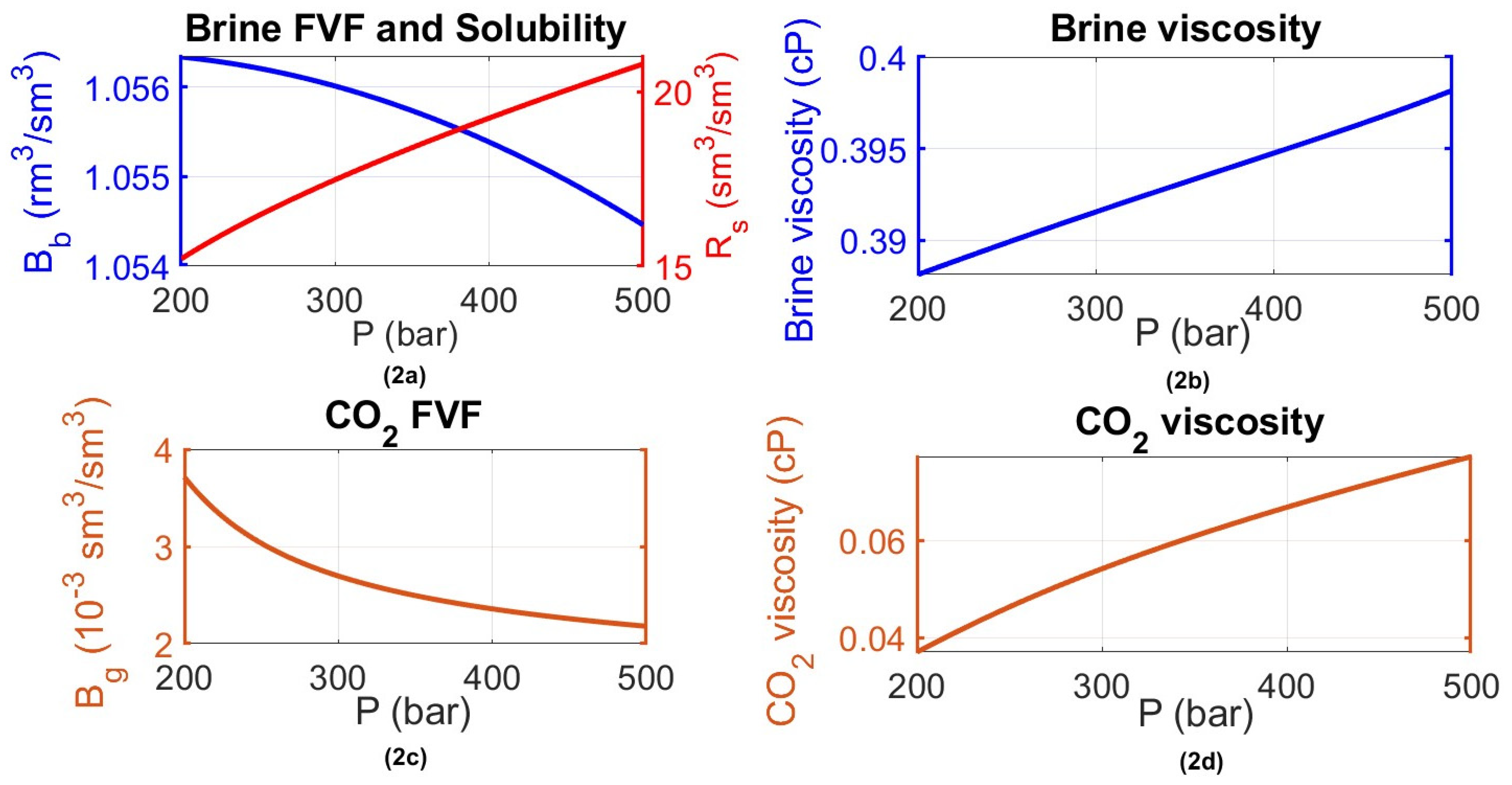
• $R_s$ (solution gas–oil ratio or CO₂–brine ratio) as a function of pressure, assessing the dissolution effect of CO₂ into brine while covering pressure levels anticipated in the reservoir ($P_{initial}$ to $P_{closure}$).
• Brine formation volume factor ($B_b$) to account for the change in the volume of the brine solution due to CO₂ solubility and therefore swelling and/or shrinking in the case of CO₂ release from the solution as a function of the reservoir pressure state.
• CO₂ formation volume factor ($B_g$) to describe the compression and expansion of the free CO₂ phase volume with a pressure change at different stages of the CCS project (injection/closure/post-closure monitoring).

Based on the above, the solution gas–oil ratio, altered to the CO₂–brine ratio and the oil formation volume factor altered to the brine FVF are defined as follows:

$$R_s=\frac{V_{dC{O}_2}^{sc}}{V_b^{sc}}$$

(46)

$$B_b=\frac{V_b^{res}}{V_b^{sc}}=\frac{V_{dC{O}_2}^{res}+V_b^{res}}{V_b^{sc}}$$

(47)

where $V_{dC{O}_2}^{sc}$ and $V_{dC{O}_2}^{res}$ are the volumes of dissolved CO₂ in the formation brine at standard and reservoir conditions (P and T), respectively, and $V_b^{sc}$ and $V_b^{res}$ are the formation brine volumes at standard and reservoir conditions, respectively. Reforming Equations (46) and (47) to be expressed in terms of phase composition/equilibrium properties obtained from the thermodynamic model described in Section 2, the solution gas–oil ratio, herein CO₂ solubility, and the formation volume factor describing brine shrinkage/swelling due to CO₂ release or dissolution are presented after Hassanzadeh et al., 2008 [34] as follows:

$$R_s=\frac{V_{dC{O}_2}^{sc}}{V_b^{sc}}=\frac{{{\overline{\rho }}_{ }}_b^{sc}{x}_{C{O}_2}}{{\overline{\rho }}_{C{O}_2}^{sc}(1-x_{C{O}_2})}$$

(48)

$$B_b=\frac{V_b^{res}}{V_b^{sc}}=\frac{{\rho }_b^{sc}}{{\rho }_b^{res}(1-{\omega }_{C{O}_2})}$$

(49)

Here, ${{\overline{\rho }}_{ }}_b^{sc}$ and ${\overline{\rho }}_{C{O}_2}^{sc}$ are the formation brine and CO₂ molar density at standard conditions, $x_{C{O}_2}$ is the CO₂ mole fraction in the aqueous phase, ${\rho }_b^{sc}$ and ${\rho }_b^{sc}$ are the formation brine mass density at standard and reservoir conditions, respectively, and ${\omega }_{C{O}_2}$ is the CO₂ mass fraction in the aqueous phase. With these equations and the thermodynamic model (solubility model) presented in Section 2, the PVT data package includes the gas–oil ratio, herein CO₂ solubility $(R_s$), and the formation volume factor of brine ($B_b)$ as a function of pressure.

Furthermore, additional input parameters needed for a black oil simulation of carbon storage in saline aquifers are computed using sampled data or correlations. For instance, CO₂ properties such as density, herein CO₂ formation volume factor ($B_g$) as a function of pressure, and viscosity are computed using built-in functions in the MATLAB Reservoir Simulation Toolbox (MRST) [35,36], specifically “CO2props”, which embeds several member functions based on sampled data covering a pressure and temperature range of 0.1 to 400 MPa and 278 to 524 K, respectively. On the other hand, other properties needed for the brine phase, such as density and viscosity at standard conditions correlated to brine salinity, are calculated using the Rowe and Chou (1970) [37] correlation and the Kestin et al., (1981) [38] methods presented in Appendix B.

It should be noted that in cases of several-phase coexistence, such as carbon storage in depleted oil fields, the presence of additional phases such as remaining and residual oil and hydrocarbon gas necessitates a more comprehensive approach accounting for four phases and their interactions. For instance, when the oil phase in the form of remaining oil is included in the problem, the dissolution of CO₂ should be accounted for in both the formation brine and the already existing oil. In such scenarios, an extended black oil model capable of accommodating all four phases (supercritical CO₂, hydrocarbon gas, brine, and oil) and their interactions may offer a more suitable solution. Such an enhanced model would require additional PVT data inputs to accurately capture the complex thermodynamic interactions that occur when multiple phases coexist.

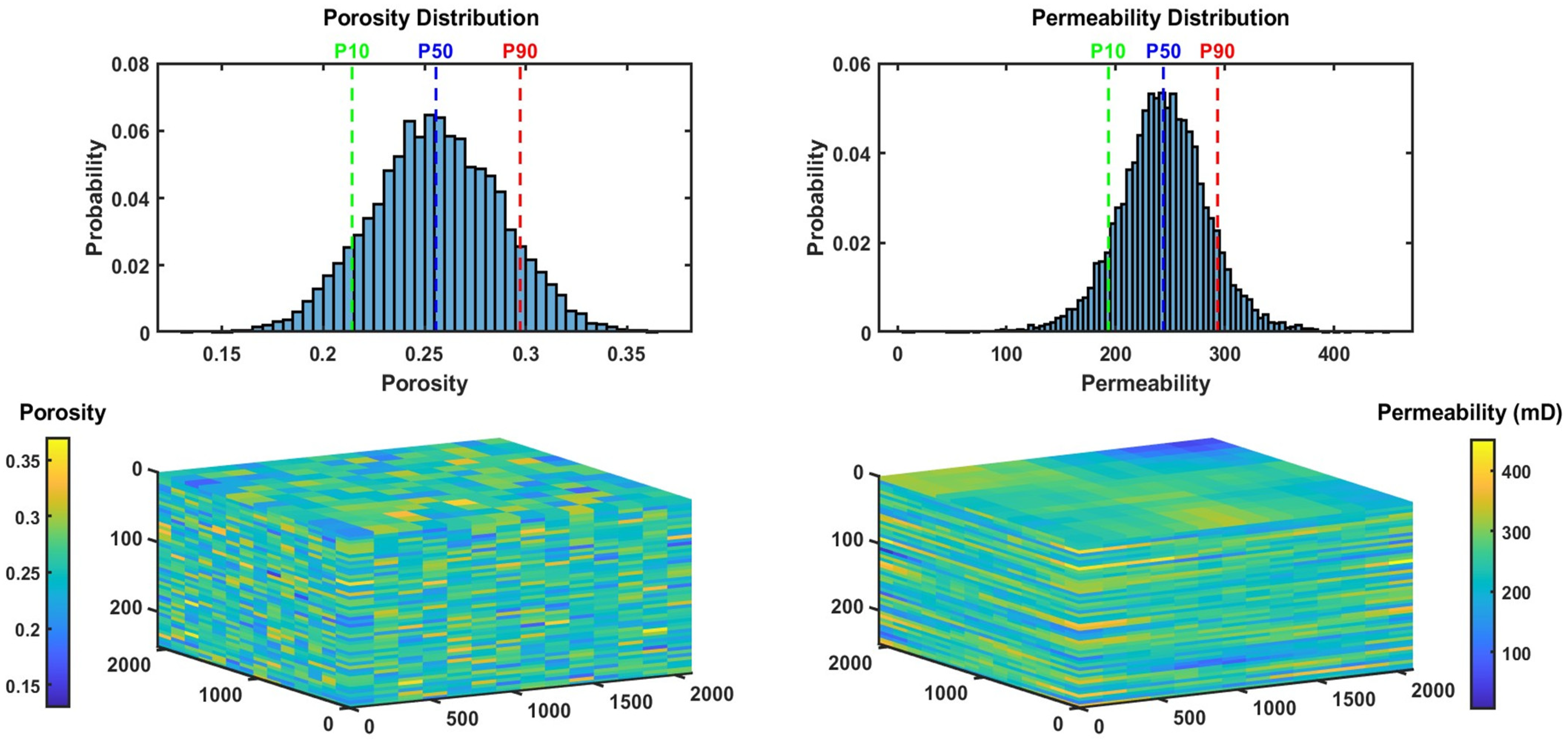
3.2. Black Oil Simulation and Generation of PVT CO₂–Brine Data: A Case Study of Typical Saline Aquifer Conditions

Overall, temperature and pressure play significant roles in determining the phase behavior of CO₂ and brine within a reservoir. Changes in temperature and pressure can alter the solubility of CO₂ in brine, affecting the extent of dissolution and thus the overall storage capacity of the reservoir. Salinity also influences the equilibrium properties by affecting the density and composition of the brine, thereby impacting the solubility of CO₂. As the solubility of the CO₂ decreases while brine salinity increases, an increase in brine salinity decreases storage efficiency due to the reduced soluble mass of CO₂ dissolved in the aqueous phase. As saline aquifers used for carbon storage are of an isothermal nature with homogeneous equilibrated salinity, pressure is typically considered to be the key factor influencing carbon storage operations and therefore simulation outcomes in carbon storage scenarios. In addition, pressure directly affects the phase behavior of CO₂, determining whether it remains in a supercritical state or transitions to a gaseous or liquid phase. Additionally, pressure variations can influence the density and compressibility of the brine, further affecting CO₂ solubility and storage capacity.

The interplay between temperature, pressure, and salinity is complex and depends on the specific geological conditions of the storage site. While pressure is commonly regarded as the predominant driver of simulation outcomes, the combined effects of temperature and salinity should also be carefully assessed to accurately predict CO₂–brine equilibrium properties in carbon storage simulations. The numerical black oil simulation in this study is conducted using the open-source MATLAB 2023a Reservoir Simulation Toolbox (MRST). The MRST provides the “CO2lab” model library tailored for carbon storage simulations, which primarily focuses on vertical equilibrium, but lacks consideration for dynamic flow processes such as fluid displacement and mixing. While efficient for assessing CO₂ migration, including the extension and migration of the CO₂ plume (containment), screening exercises, sensitivity analyses, and preliminary design decisions, it operates under the assumption of quasi-steady-state conditions presuming that pressure and density gradients stabilize relatively quickly. Therefore, for this study, the MRST black oil model originally designed for oil and gas production and full scale, fully dynamic simulation has been chosen, with necessary modifications to suit the specific requirements of simulating carbon storage in saline aquifers.

3.2.1. Black Oil Simulation: Characteristics and PVT Data

A simplified 3D Cartesian model is utilized to simulate the two-phase flow of CO₂, incorporating in-house collected characteristics observed in significant commercial projects worldwide which offer a thorough representation of the current progress in CCS and are summarized in

Table 4. Summary of Key Characteristics of Large-Scale Commercial Projects.

Project Name	Location	Inj. Start	Aquifer Unit (Lithology)	Average Porosity	Average Permeability	Depth	Thickness (m)	Temperature (ICI)	Pressure (MPa)
Snohvit	Barents Sea, Norway	2008	Tubasen Formation (Sandstone)	13	450	2550	60	95	28.5
Sleipner	North Sea, Norway	1996	Utsira Formation (Sandstone)	37	5000	1000	250	37	10.3
In Salah	Krechba, Algeria	2004	Krechba Formation (Sandstone)	17	5	1850	29	90	17.9
Gorgon	Barrow Island, WA, Australia	2014	Dupuy Formation (Sandstone)	20	25	2300	N/A	100	22

. The simulated aquifer spans 2100 m in both length and width, with a maximum observed thickness of 250 m. The grid resolution is set to 150 m in the x and y directions and 5 m in the z direction, resulting in a grid configuration of 14 × 14 × 50 cells. The reservoir exhibits Gaussian distributed heterogeneity, with porosity ranging from 13% to 37% and permeability ranging from 5 to 450 mD covering the spectrum observed in large-scale commercial projects except for the Sleipner case, which features a specific permeability of 5 Darcy. Figure 1 illustrates the distribution of these properties, offering insights into reservoir heterogeneity.

The top reservoir is positioned at a depth of 1925 m derived from the weighted average of all cases. The reservoir is assumed to be horizontally layered and therefore isothermal, with a maximum observed temperature of 100 °C. In addition, in the absence of publicly available salinity data, a salinity of 150,000 ppm is adopted, referencing the L. Tuscaloosa Sandstone Formation in the SECARB Mississippi Pilot project [39]. This results in a top pressure of 206.1 bars, correlated to a brine standard density of 1092 kg/m³ and a reservoir density of 1057 kg/m³. Additionally, the rock compressibility is assumed at 40 × 10⁻⁷ (1/psi), and relative permeabilities are produced using a connate water saturation of 0.27 and a residual CO₂ saturation of 0.20, utilizing built-in functions of MRST.

The primary PVT data for black oil modeling, including the solution gas–oil ratio altered to the CO₂–brine ratio and the oil formation volume factor altered to brine, are produced as functions of pressure for the aquifer with the specified characteristics (T = 100 °C and salinity of 150,000 ppm) using Equations (48) and (49), in combination with the solubility model discussed in Section 2. The brine density at standard conditions and reservoir viscosity are determined from correlations discussed before, while the standard density, reservoir viscosity as well as CO₂ formation volume factor tables are determined using the MRST CO2prop built-in functions. Figure 2 summarizes the main PVT data parameters produced and utilized when simulating carbon storage in the described aquifer. Additionally,

Table 5. PVT parameters introduced.

Parameter	Value
Standard brine density	1092 kg/m3
Standard CO2 density	1.8 kg/m3
Average brine viscosity	0.393 cp
Average CO2 viscosity	0.06 cp

provides an overview of the standard input PVT parameters introduced and the approximation of viscosity data.

Two injection wells were situated on one side of the reservoir (XY: 1,1 and 1,14), while two producers were positioned on the opposite side (XY: 14,1 and 14,14). Each injector was set to be rate-controlled, injecting 0.5 million tons per annum (0.5 Mtpa) into the last three layers (48:50), corresponding to a 15 m long perforation. A constraint was imposed on the bottom hole pressure of 500 bars, aligning with the maximum pressure buildup allowed. Conversely, the producers were configured to extract brine to alleviate pressure buildup, facilitating more efficient carbon injection and storage. Thus, they were set to be rate controlled at 2550 stb/day each and perforated in the last three layers (15 m) to minimize the production of CO₂.

The simulation encompassed a typical injection period of 25 years, corresponding to the standard duration for storage operation permits, followed by a 75-year post-closure monitoring phase, resulting in a total simulation time of 100 years. During the operational phase, the simulation employed a monthly time step to yield results, whereas during the post-closure period, it utilized quarterly intervals thanks to the significantly lower pressure and saturation change rate during equilibrium.

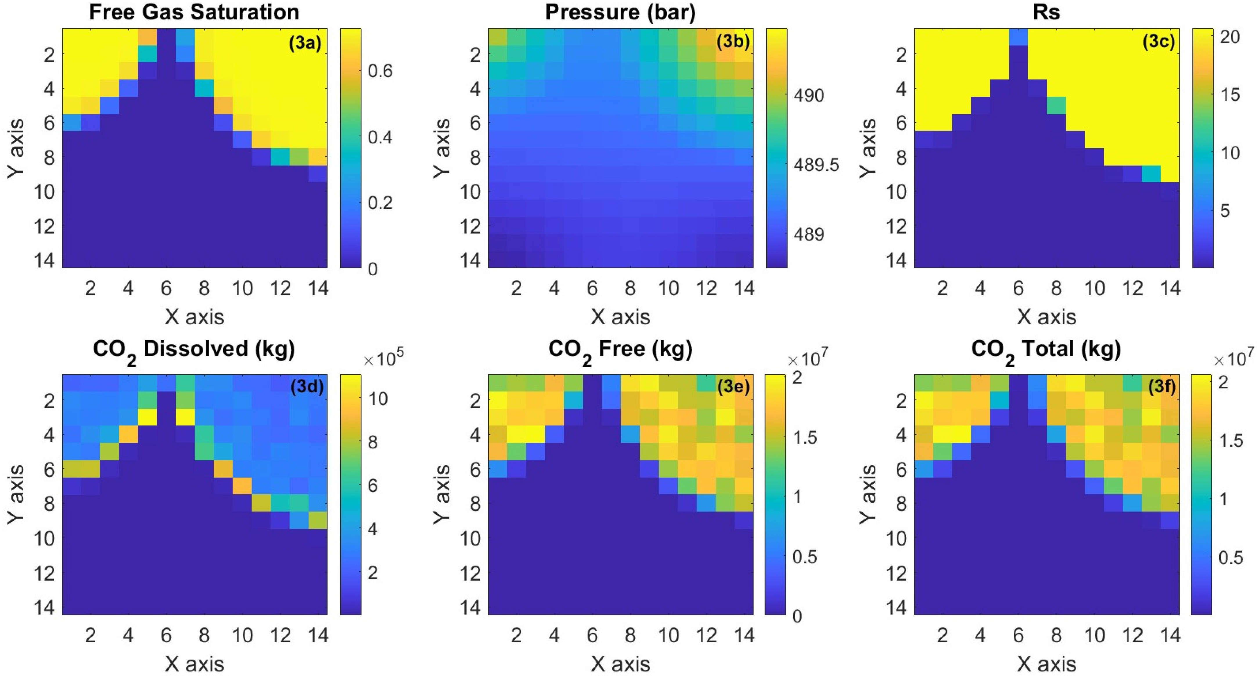
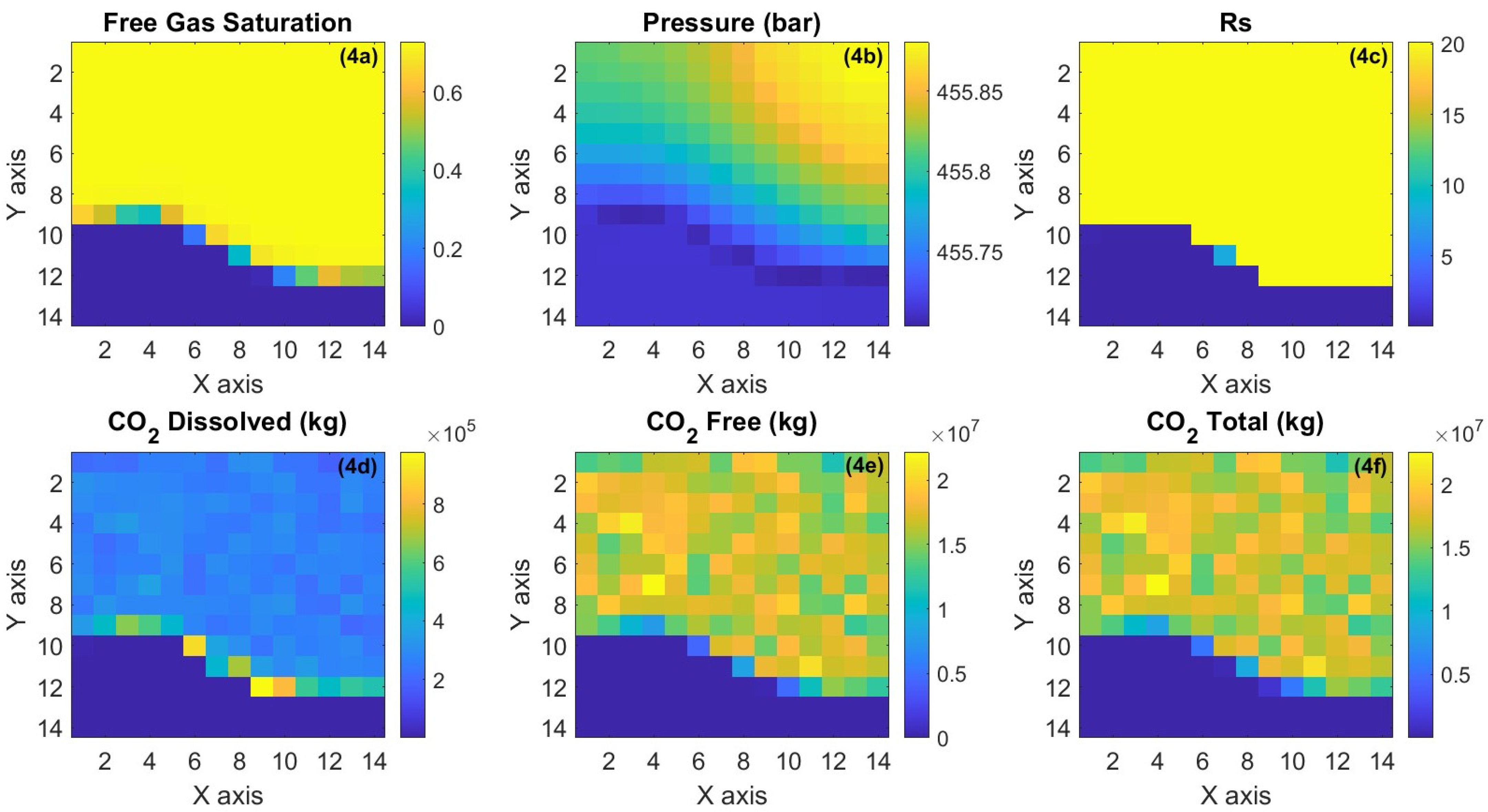
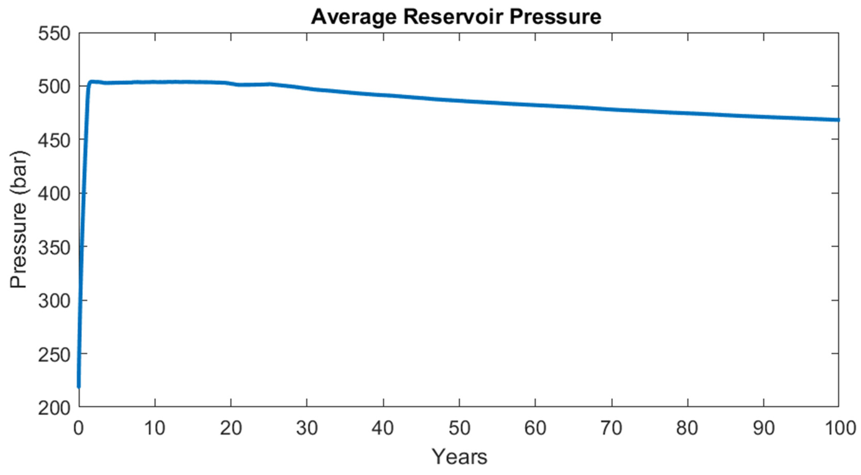
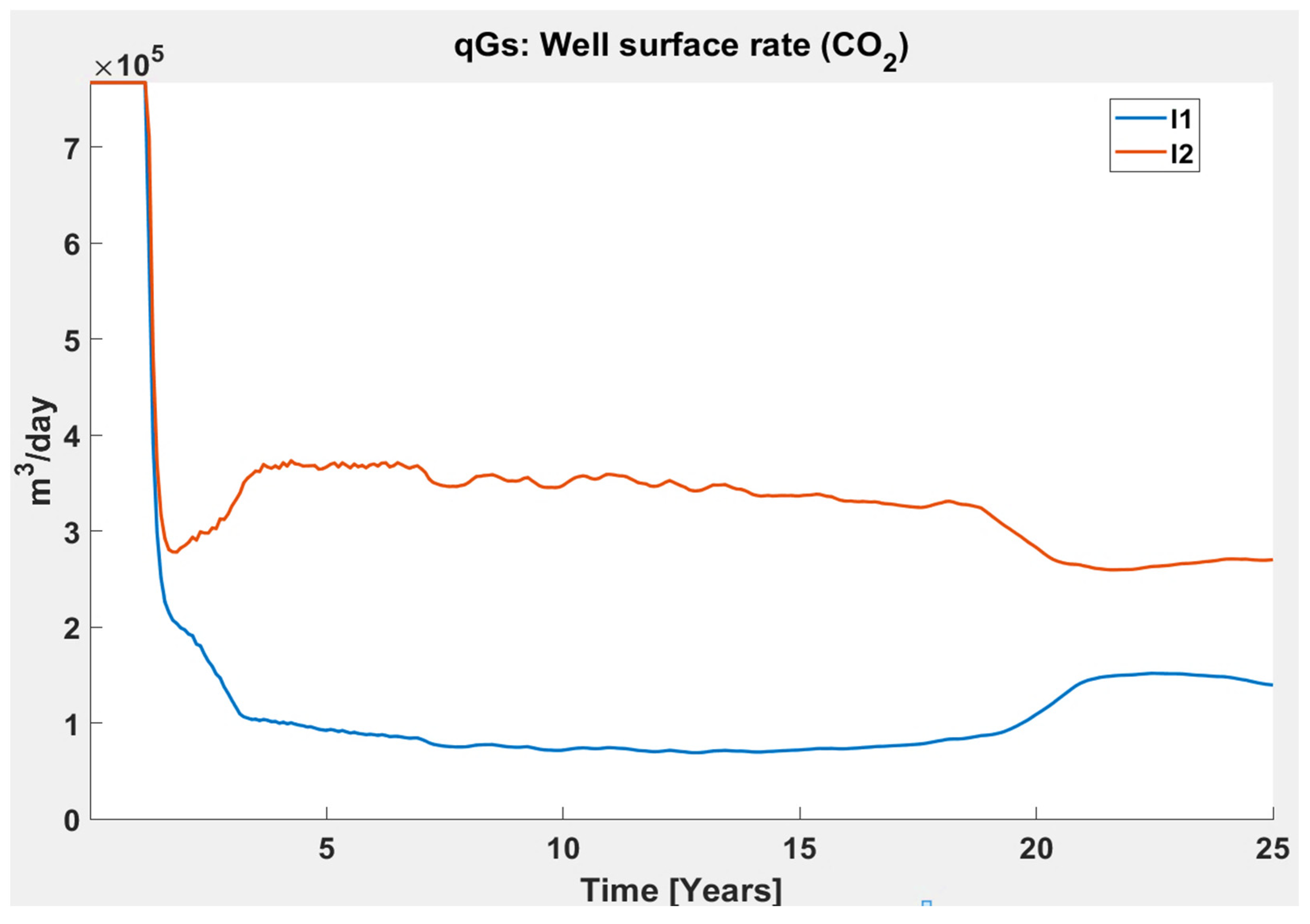
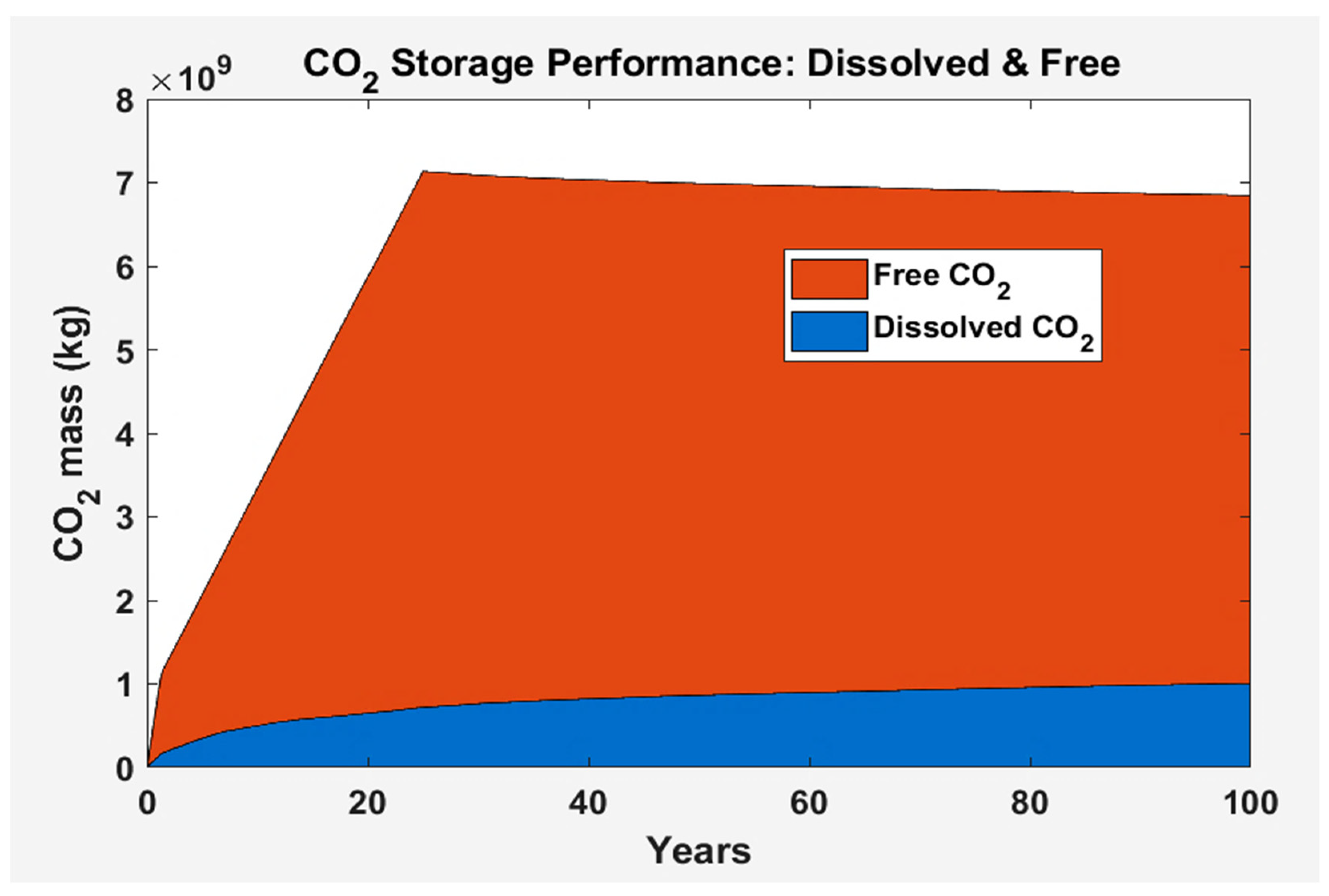
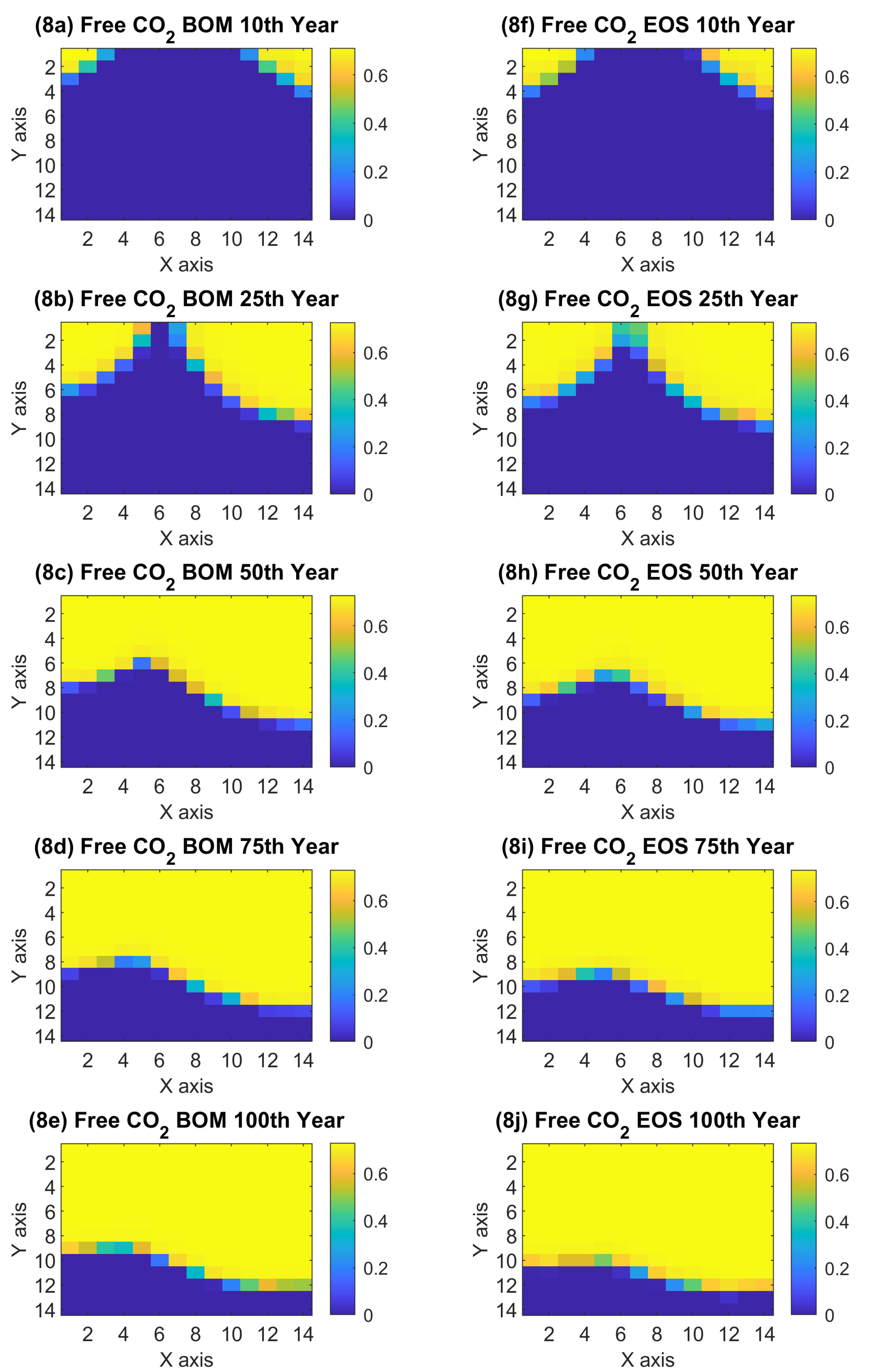
3.2.2. Black Oil Simulation: Results

To comprehensively evaluate the simulation outcomes, we conducted an exhaustive analysis of a diverse array of datasets. Our primary focus was on tracking the extension of the CO₂ plume by examining free gas saturation, along with other parameters crucial for understanding plume extension in carbon storage. This assessment is vital for ensuring the containment of CO₂ within the storage site and preventing migration to surrounding areas. Additionally, we evaluated the pressure profile in conjunction with the dissolution and free gas trapping profiles. Understanding these parameters is essential for assessing site integrity, conducting safety evaluations, and performing long-term risk assessments for potential CO₂ leakage.

Figure 3 provides a detailed depiction of the key information used to monitor the migration of the CO₂ plume, pressure distribution, and dissolution phenomenon profile. It also illustrates the overall simulation results in terms of CO₂ mass entrapped in each form (dissolved and free) at the conclusion of the operational phase (after 25 years of injection) for the uppermost layer of the reservoir. Due to reservoir heterogeneity and maximum capped pressure, the two corner wells inject differently, resulting in the formation of two separate plumes that mimic real-world gas distribution among different reservoir regions. This visualization offers a clear picture into how CO₂ behaved within this layer over time, enhancing our understanding of the effectiveness of the black oil simulation technique in capturing its distribution, movement, and potential impact on the storage site and surrounding environment. In Figure 3, the saturation distribution (3a) at the conclusion of the injection phase in both plumes reveals a predominant saturation of free gas (CO₂ “gas cap”), with a saturation value exceeding 0.70. This is complemented by a saturation value of 0.27 representing the connate/irreducible water saturation. As we progress through the tails and intermediate regions, the prevalence of free gas saturation persists, gradually transitioning towards the plume interface and forefront. A notable decline in saturation is observed in both plumes, ranging from 0.05 to 0.6, signifying the forefront of the plume’s migration. Within this observation, it is clear that the black oil simulation effectively captures the buoyancy effect, the gradual transition of free gas saturation along the plume interface, and the forefront. These aspects are interconnected with the solubility effect and convection mechanisms occurring in underground carbon storage.

On top of the observed distribution of saturation, the pressure distribution (3b) within the reservoir layer exhibits a distinct pattern, revealing a smooth transition in pressure correlated with slight variations in free gas saturation. In the topmost layer saturated with free gas CO₂ (referred to as the “CO₂ gas cap”), the pressure is relatively high near the injectors (tail of the CO₂ plume) due to the accumulation of CO₂ gas in its supercritical state, with a saturation of approximately 0.73. Meanwhile, a gradual transition in pressure is correlated with slight variations in the saturation of free gas (ranging from 0.70 to 0.73). Conversely, in regions where the saturation of CO₂ decreases, such as at the forefront interface of the plume, the pressure is lower compared to the gas-saturated areas. This decrease is attributed to the dissolution of CO₂ into the brine phase, resulting in a reduction in gas volume and consequently a pressure reduction, with the lowest pressure observed around the producers. Overall, the pressure distribution obtained using the black oil model, which is closely correlated to formation volume factors input tables, reflects the dynamic interplay between gas saturation, dissolution effects, and the movement of the CO₂ plume within the reservoir.

When examining the distribution of $R_s$ (3c), or the gas–brine ratio within the reservoir, an expected gradient correlated with pressure is observed. In the topmost layer, where the pressure variation is minimal, $R_s$ (the solubility parameter) demonstrates a coherent distribution, with values approximately around 20 sm³/m³ in the tail and intermediate regions of the CO₂ plume. Moreover, the $R_s$ values accurately portray the solubility in blocks already contacted with CO₂, mirroring the block pressure. In blocks where no CO₂ has been contacted but the pressure is relatively similar or close enough, $R_s$ accurately depicts a value of 0, indicating a precise correlation to both phases and pressures. Within the forefront interface blocks of both plumes (e.g., blocks: 1,6; 2,6 and 8,4; 14,9, etc.), the $R_s$ values reach their maximum, while free gas saturation varies. This observation indicates an accurate representation of the plume’s evolution: as CO₂ contacts fresh brine, it undergoes dissolution, and after full brine saturation with CO₂, the free gas phase begins to form. Additionally, focusing on blocks like 6,1 (interface of both plumes), 5,1; 14,9; 13,9; 12,9, etc., different $R_s$ values are evident with a gas saturation equal to 0. This suggests that CO₂ has reached these blocks; however, “first & multiple contact solubility” took place with different solubility values correlated to the amount of CO₂ reached in each block, with no free gas formed. Observations of $R_s$ signify the dynamic interaction between solubility, gas saturation, and pressure within the reservoir, providing insights into the capability of black oil simulation to accurately mimic various in-situ phenomena and behaviors of injected CO₂.

On the other hand, analyzing the output value projection regarding CO₂ mass dissolved (3d), free (3e), and total CO₂ stored in the reservoir (3f) unveils a significant variation in the trapped CO₂ between dissolution and free gas across different blocks in the uppermost layer. The contrast in the magnitude of trapped CO₂ is striking, with dissolved CO₂ being on the order of magnitude of 10⁵, while free gas is approximately 10⁷, confirming the expectation of relatively low dissolution trapping compared to free gas. Moreover, the consistent variation in trapped mass among different blocks arises from a combination of factors. Primarily, inherent rock properties play a crucial role, including heterogeneity in permeability and porosity. This heterogeneity leads to a variation in void volumes available, alterations in the mass of connate water, and creates different “thief” paths for CO₂ to flow. Additionally, slight variations in PVT properties among the blocks, such as $R_s$, contribute minimally to the observed differences.

A similar interpretation and analysis can be extended to Figure 4, illustrating similar key information, monitoring the migration of a continuous CO₂ plume (the segregation/integration of the two plumes), the dissolution phenomenon, and the overall simulation results over 100 years (25 years of injection with 75 years of post-closure monitoring). Notably, the black oil simulation demonstrates the expected equilibrated pressure propagation among the top layer at the end of the simulation time (100 years), despite the two plumes separately exhibiting distinct pressure profiles at the end of the injection as shown in Figure 3.

Evaluating the second set of data, which includes the pressure profile along with the dissolution and free gas trapping profiles, is essential for assessing the capability of the black oil model technique as a representative tool in the assessment of site integrity through accurate pressure prediction (thereby mitigating pressure buildup and potential geomechanical complications) and relatively short-term risk assessment (e.g., 25 years injection). In addition, long-term risk assessments for potential CO₂ leakage from the storage site are closely correlated to the amount of CO₂ stored in mobile form, which is more prone to leak than any other form. Therefore, the capability of the black oil model in accurately representing and distinguishing carbon stored within low-risk mechanisms such as dissolution versus relatively higher-risk mechanisms such as mobile CO₂ plumes is crucial from both operational and regulatory perspectives.

Figure 5 illustrates the average reservoir pressure over the injection and monitoring phases. When examining the average reservoir pressure profile depicted in Figure 5, three distinct patterns emerge. The first pattern corresponds to the injection period, spanning approximately from year 0 to 2 years, while the second pattern covers the interval from 2 to 25 years. The third pattern represents the overall monitoring phase from 25 to 100 years.

In the initial period (0–2 years), the reservoir continues to “inflate” as expected, attributed to the higher downhole volume of the injected fluid compared to the withdrawn brine. By approximately 2 years, the bottom hole pressure constraints of the injectors are activated, leading to a reduction in injection rates and a constant pressure for the remainder of the injection period (2–25 years). Figure 6 accurately depicts this constraint, showcasing the adjustment of injection rates to meet constraints imposed on the injectors’ bottom hole pressure, ensuring it does not exceed the specified value (500 bars). The disparity in observed injection rates between Injector 1 and Injector 2 is attributed to the asymmetry in the petrophysics of the reservoir regions where each injector is situated, including variations in porosity and permeability.

Starting at the 25-year mark and extending beyond (up to 100 years), a continuous decline in average reservoir pressure is evident. This decrease is associated with the extended expansion of the CO₂ plume within the reservoir and the attainment of equilibrium over the very long term (e.g., 1000 years). As the plume traverses the reservoir, additional dissolution of CO₂ occurs upon contact with “fresh” undersaturated brine. This ongoing movement of CO₂ results in further dissolution, leading to a reduction in the presence of the free gas phase (free gas/dense phase saturation). Figure 7 illustrates that after the cessation of injection at the 25-year mark, free gas CO₂ diminishes, while the reservoir concurrently experiences a proportional increase, adhering to mass conservation principles. This trend supports the observed decrease in average reservoir pressure during the post-closure monitoring phase.

Overall, based on the results observed during both the injection and monitoring phases, it can be concluded that the black oil model technique effectively captures the movement of the CO₂ plume during post-closure monitoring, where no dynamic injection takes place. It accurately represents the dissolution of CO₂ in undersaturated brine, further reducing the presence of the dense mobile phase in the reservoir.

4. Performance Comparison between Black Oil Model and Compositional Model

In this Section, our objective is to bolster the credibility of the black oil model as a reliable tool for simulating carbon storage by comparing its results to those of a conventional compositional model. By utilizing the compositional model as a benchmark, we assess the outcomes of the black oil model presented in Section 3. Similar to the previous Section, we analyze the free gas saturation (plume expansion) in the topmost layer of the reservoir generated by both the black oil simulation (BoM) and the compositional model (EoS). The significance of examining plume extension stems from its crucial role in evaluating the safety and efficiency of carbon storage operations. This includes containing the mobile CO₂ injected within the storage site/formation to prevent any leakage into the surrounding environments, such as storage complexes, and managing the primary risks and challenges associated with potential leakage through open fractures and conduits that could be encountered in the storage formation. To achieve this, we employ the Eclipse E300 compositional [40] commercial simulator to simulate the same case discussed previously. Figure 8 illustrates the results of the free CO₂ plume in the topmost aquifer layer (layer number 1) and compares the outcomes obtained using the BoM developed in this work with those obtained using Eclipse E300 model.

At simulation time T = 10 years, the results indicate that the BoM (8a) slightly underestimates the expansion of the plume compared to the EoS results (8f). However, when it comes to the extent of the plume, the discrepancy between the black oil model and the compositional one averages about one block (~150 m) in both directions x and y. To further assess this difference, the left-hand side plume forefront interface is examined. It is observed that in the x direction, the EoS model shows the plume forefront interface reaching block 4,1, whereas the black oil model simulation indicates that the interface is still at block 3,1. Similarly, in the y direction, the BoM plume reaches block 1,3 while the EoS one reaches block 1,4. Furthermore, similar results are obtained by the end of the injection time (T = 25), further confirming that the spatial difference between BoM and EoS analyses in capturing the extent of the plume in the reservoir is on the order of 150 m. During the monitoring phase (post-closure, T = 50 (8c), 75 (8d), and 100 years (8e)), the consistency between the results of both techniques (BoM and EoS) is also similar to the operational period results. Whereas during the injection period, a discrepancy of one block or 150 m is depicted between both models, and the same applies for the monitoring phase where a similar minor discrepancy is noticed.

The pattern of difference observed between the black oil model and the compositional model can be attributed to several factors. During the injection/operational period, where the black oil model shows a discrepancy of one block (150 m) compared to the EoS model results are obtained by T = 10 and 25 years (8a and 8b, respectively), this difference is likely due to the highly buoyant nature of CO₂ during injection. The pressure plume/drive mechanisms generated from the continuous injection of CO₂, coupled with the relatively rapid phase equilibrium changes at the plume interface, are better captured by the compositional model due to its inherent ability to calculate phase equilibrium and track phase composition accurately. Additionally, when such a pattern is still observed in the monitoring phase where no such high buoyancy and drive mechanism is expected, particularly at 100 years, the black oil model continues to show a similar difference to the one seen in the results of the operation/injection period (10 and 25 years). Therefore, it can be said that such a difference cannot only be attributed to the modeling technique itself, but also to the discretization/block size, indicating the need for a finer grid in both the x and y directions when employing black oil model technique, as will be explored in a later part of this study, to accurately capture the plume extent. In addition to the above, the sensitivity of the black oil model input parameters produced in this work using solubility models and representative equations (Section 2 and Section 3), except case-specific lab data, could also contribute to very minor discrepancies between the black oil model and the compositional model results.

Overall, for evaluating the extent of the plume and assessing the safety of carbon storage operations within a specific formation or site, the black oil model proves to be a reliable tool that serves the intended purpose effectively.

To further evaluate the capability of the BoM technique in simulating carbon storage operations, we assess the average pressure and dissolution/free rates of both fluid modeling techniques over the entire simulation period of 100 years. Reservoir pressure is a critical parameter for assessing the risk of pressure buildup in the formation and caprock, which could lead to the fracturing of both carbon storage elements if the pressure exceeds certain thresholds (e.g., fracture pressure). Additionally, security assessments of storage in terms of the mass fraction of carbon stored in dissolution and free gas forms are crucial in assessing long-term containment. Figure 9 illustrates the average reservoir pressure profile as well as the dissolution and free mass fraction rates over the total simulation time of 100 years (25 years of injection and 75 years of post-closure monitoring). The fraction rate corresponds to the mass of CO₂ stored in the form of a corresponding mechanism (e.g., dissolution) over the total CO₂ mass stored at each time step.

Considering the results of the average pressure profile obtained from both the BoM and compositional techniques, it is observed that the BoM approach tends to slightly overestimate the average pressure in the reservoir during the injection period and for some parts of the monitoring phase. While the EoS model predicts an average pressure of approximately 490 bars, the BoM prediction is slightly higher at 500 bars, reflecting a relative difference of approximately 2% up to 60 years of simulation. However, as the reservoir begins to equilibrate after 25 years, the average reservoir pressure starts to decline, eventually converging to that of the EoS model by the end of the 100-year simulation period. This behavior is attributed to the high buoyancy and pressure plume during the injection period, which is better captured through compositional phase equilibria, albeit with higher computational demand and complexity. Overall, the average absolute relative difference in average reservoir pressure using the BoM technique is approximately 3.85% over the entire simulation time, representing a minor deviation. This further strengthens the employment of the black oil fluid modeling technique as a viable option to simulate carbon storage, even though it slightly overestimates the average pressure in the reservoir.

On the other hand, when considering the dissolution and free gas rates or the mass fraction, it is noticed that the black oil simulation slightly underestimates the dissolution rate or the mass fraction, with the complementary factor being the free CO₂/mobile CO₂. The difference of both fluid modeling techniques shows a consistent gap trend of difference. This is consistent with the average since a higher dissolution effect against the free gas plume implies lower pressure due to the higher density of the dissolved CO₂ compared to that of the supercritical free phase. Additionally, such minor differences should be partially attributed to the block size itself, suggesting that a further decrease in the block size (possibly in the x and y direction) to less than 150 m could show a higher consistency (possibly < 4% difference), further strengthening the capability of the BoM technique in simulating carbon storage operations.

5. Discussion

The integration of black oil modeling into carbon storage simulations marks a significant advancement in carbon mitigation strategies. Leveraging techniques from the oil and gas industry, particularly the black oil model (BoM), our study introduced an alternative approach to simulating carbon storage in saline aquifers and achieving efficient decision-making. This methodology tackled key challenges in CCS, such as computational complexity, while ensuring accuracy and reliability. We incorporated a solubility thermodynamic model capable of predicting CO₂–brine equilibrium properties offline, reducing computational overhead. This enhanced model can accommodate various salts up to a concentration of 4.3 m and extends to pressure and temperature ranges suitable for both carbon storage in saline aquifers in moderate and “hot” basins, thus finding application in Enhanced Geothermal Systems.

In our work, we developed and tested the solubility model for a saline aquifer with specific characteristics. PVT data generated using this model were then introduced into the simulator, and carbon storage simulations using the BoM technique were conducted. The results aligned with expectations. When compared to compositional modeling, the BoM showed strong agreement with minor differences in plume extent and average reservoir pressure, reducing CPU time to at least one-fourth of that of a compositional model. However, further analyses suggested that these differences were likely attributed to grid block size/dimension rather than the model itself.

Moving forward, several avenues for further research emerge. Firstly, the applicability of the black oil model when taking into consideration different geological setting (e.g., a depleted oil field) should be further assessed in further research. In addition, while the aim of this work is to lay the foundation for the application of the black oil model in the CCS domain, this study did not explicitly address grid discretization and resolution effects and their implications on simulation outcomes such as grid shape, resolution, and orientation which can significantly influence the shapes and extents of free CO₂ plumes. For instance, coarse vertical discretization of a reservoir may hinder gravity override, potentially underestimating the maximum plume size. Therefore, future research should address the impact of grid discretization and resolution in all three directions (x, y, and z) on result accuracy when applying the BoM. Additionally, comparing the BoM’s performance with Vertical Equilibrium simulations could elucidate the additional computational costs incurred when applying full dynamic modeling, assessing trade-off between accuracy and computational cost. The authors intend to address these aspects in a future extension of this work, alongside the application of optimization techniques for well allocation and strategies while employing the BoM. Lastly, exploring the application of the solubility model in geothermal systems is another area of research interest, aiming to accurately model the density and solubility phenomena involved in CO₂ Plume Geothermal (CPG) applications.

Overall, this research demonstrates the potential of the BoM technique in carbon storage simulations and lays the groundwork for further investigations into its application and optimization. By addressing these research gaps, we aim to enhance the efficiency and effectiveness of carbon storage strategies, contributing to global efforts to mitigate CO₂ emissions and combat climate change.

References

1. Jarvis, S.M.; Samsatli, S. Technologies and Infrastructures Underpinning Future CO2 Value Chains: A Comprehensive Review and Comparative Analysis. Renew. Sustain. Energy Rev. 2018, 85, 46–68. [Google Scholar] [CrossRef]
2. Gabrielli, P.; Gazzani, M.; Mazzotti, M. The Role of Carbon Capture and Utilization, Carbon Capture and Storage, and Biomass to Enable a Net-Zero-CO2 Emissions Chemical Industry. Ind. Eng. Chem. Res. 2020, 59, 7033–7045. [Google Scholar] [CrossRef]
3. Bui, M.; Gazzani, M.; Pozo, C.; Puxty, G.D.; Soltani, S.M. Editorial: The Role of Carbon Capture and Storage Technologies in a Net-Zero Carbon Future. Front. Energy Res. 2021, 9, 733968. [Google Scholar] [CrossRef]
4. Martin-Roberts, E.; Scott, V.; Flude, S.; Johnson, G.; Haszeldine, R.S.; Gilfillan, S. Carbon Capture and Storage at the End of a Lost Decade. One Earth 2021, 4, 1569–1584. [Google Scholar] [CrossRef]
5. Peres, C.B.; Resende, P.M.R.; Nunes, L.J.R.; Morais, L.C.D. Advances in Carbon Capture and Use (CCU) Technologies: A Comprehensive Review and CO2 Mitigation Potential Analysis. Clean Technol. 2022, 4, 1193–1207. [Google Scholar] [CrossRef]
6. Li, Q.; Liu, J.; Wang, S.; Guo, Y.; Han, X.; Li, Q.; Cheng, Y.; Dong, Z.; Li, X.; Zhang, X. Numerical Insights into Factors Affecting Collapse Behavior of Horizontal Wellbore in Clayey Silt Hydrate-Bearing Sediments and the Accompanying Control Strategy. Ocean. Eng. 2024, 297, 117029. [Google Scholar] [CrossRef]
7. International Energy Agency. Putting CO2 to Use; International Energy Agency: Paris, France, 2019. [Google Scholar]
8. Ji, X.; Zhu, C. Aquifers. In Novel Materials for Carbon Dioxide Mitigation Technology; Elsevier: Amsterdam, The Netherlands, 2015; pp. 299–332. [Google Scholar] [CrossRef]
9. Hannis, S.; Lu, J.; Chadwick, A.; Hovorka, S.; Kirk, K.; Romanak, K.; Pearce, J. CO2 Storage in Depleted or Depleting Oil and Gas Fields: What Can We Learn from Existing Projects? Energy Procedia 2017, 114, 5680–5690. [Google Scholar] [CrossRef]
10. Gassara, O.; Estublier, A.; Garcia, B.; Noirez, S.; Cerepi, A.; Loisy, C.; Le Roux, O.; Petit, A.; Rossi, L.; Kennedy, S.; et al. The Aquifer-CO2Leak Project: Numerical Modeling for the Design of a CO2 Injection Experiment in the Saturated Zone of the Saint-Emilion (France) Site. Int. J. Greenh. Gas. Control 2021, 104, 103196. [Google Scholar] [CrossRef]
11. Michael, K.; Allinson, G.; Golab, A.; Sharma, S.; Shulakova, V. CO2 Storage in Saline Aquifers II–Experience from Existing Storage Operations. Energy Procedia 2009, 1, 1973–1980. [Google Scholar] [CrossRef]
12. Pruess, K.; García, J.; Kovscek, T.; Oldenburg, C.; Rutqvist, J.; Steefel, C.; Xu, T. Code Intercomparison Builds Confidence in Numerical Simulation Models for Geologic Disposal of CO2. Energy 2004, 29, 1431–1444. [Google Scholar] [CrossRef]
13. Class, H.; Ebigbo, A.; Helmig, R.; Dahle, H.K.; Nordbotten, J.M.; Celia, M.A.; Audigane, P.; Darcis, M.; Ennis-King, J.; Fan, Y.; et al. A Benchmark Study on Problems Related to CO2 Storage in Geologic Formations. Comput. Geosci. 2009, 13, 409–434. [Google Scholar] [CrossRef]
14. Ismail, I.; Gaganis, V. Carbon Capture, Utilization, and Storage in Saline Aquifers: Subsurface Policies, Development Plans, Well Control Strategies and Optimization Approaches—A Review. Clean Technol. 2023, 5, 609–637. [Google Scholar] [CrossRef]
15. Blair, L.M.; Quinn, J.A. Measurement of Small Density Differences: Solutions of Slightly Soluble Gases. Rev. Sci. Instrum. 1968, 39, 75–77. [Google Scholar] [CrossRef]
16. Sayegh, S.G.; Najman, J. Phase Behavior Measurements of CO2 -SO2 -brine Mixtures. Can. J. Chem. Eng. 1987, 65, 314–320. [Google Scholar] [CrossRef]
17. Lindeberg, E.; Wessel-Berg, D. Vertical Convection in an Aquifer Column under a Gas Cap of CO2. Energy Convers. Manag. 1997, 38, S229–S234. [Google Scholar] [CrossRef]
18. Ennis-King, J.; Paterson, L. Role of Convective Mixing in the Long-Term Storage of Carbon Dioxide in Deep Saline Formations. SPE J. 2005, 10, 349–356. [Google Scholar] [CrossRef]
19. Hassanzadeh, H.; Pooladi-Darvish, M.; Keith, D.W. Modelling of Convective Mixing in CO2 Storage. In Canadian International Petroleum Conference; Petroleum Society of Canada: Calgary, AB, Canada, 2004. [Google Scholar] [CrossRef]
20. Yang, Z.-L.; Yu, H.-Y.; Chen, Z.-W.; Cheng, S.-Q.; Su, J.-Z. A Compositional Model for CO2 Flooding Including CO2 Equilibria between Water and Oil Using the Peng–Robinson Equation of State with the Wong–Sandler Mixing Rule. Pet. Sci. 2019, 16, 874–889. [Google Scholar] [CrossRef]
21. Spycher, N.; Pruess, K.; Ennis-King, J. CO2-H2O Mixtures in the Geological Sequestration of CO2. I. Assessment and Calculation of Mutual Solubilities from 12 to 100 °C and up to 600 Bar. Geochim. Cosmochim. Acta 2003, 67, 3015–3031. [Google Scholar] [CrossRef]
22. Spycher, N.; Pruess, K. CO2-H2O Mixtures in the Geological Sequestration of CO2. II. Partitioning in Chloride Brines at 12–100 °C and up to 600 Bar. Geochim. Cosmochim. Acta 2005, 69, 3309–3320. [Google Scholar] [CrossRef]
23. Spycher, N.; Pruess, K. A Phase-Partitioning Model for CO2–Brine Mixtures at Elevated Temperatures and Pressures: Application to CO2-Enhanced Geothermal Systems. Transp. Porous Media 2010, 82, 173–196. [Google Scholar] [CrossRef]
24. Duan, Z.; Sun, R. An Improved Model Calculating CO2 Solubility in Pure Water and Aqueous NaCl Solutions from 273 to 533 K and from 0 to 2000 Bar. Chem. Geol. 2003, 193, 257–271. [Google Scholar] [CrossRef]
25. Duan, Z.; Sun, R.; Zhu, C.; Chou, I.-M. An Improved Model for the Calculation of CO2 Solubility in Aqueous Solutions Containing Na+, K+, Ca2+, Mg2+, Cl, and SO42−. Mar. Chem. 2006, 98, 131–139. [Google Scholar] [CrossRef]
26. Tödheide, K.; Franck, E.U. Das Zweiphasengebiet Und Die Kritische Kurve Im System Kohlendioxid–Wasser Bis Zu Drucken von 3500 Bar. Z. Für Phys. Chem. 1963, 37, 387–401. [Google Scholar] [CrossRef]
27. Takenouchi, S.; Kennedy, G.C. The Binary System H2O-CO2 at High Temperatures and Pressures. Am. J. Sci. 1964, 262, 1055–1074. [Google Scholar] [CrossRef]
28. Blencoe, J.G.; Naney, M.T.; Anovitz, L.M. The CO2–H2O System: III. A New Experimental Method for Determining Liquid-Vapor Equilibria at High Supercritical Temperatures. Am. Mineral. 2001, 86, 1100–1111. [Google Scholar] [CrossRef]
29. Hu, J.; Duan, Z.; Zhu, C.; Chou, I.-M. PVTx Properties of the CO2–H2O and CO2–H2O–NaCl Systems below 647 K: Assessment of Experimental Data and Thermodynamic Models. Chem. Geol. 2007, 238, 249–267. [Google Scholar] [CrossRef]
30. Fotias, S.P.; Bellas, S.; Gaganis, V. Optimizing Geothermal Energy Extraction in CO2 Plume Geothermal Systems. Mater. Proc. 2023, 15, 52. [Google Scholar] [CrossRef]
31. Mathias, P.M.; Klotz, H.C.; Prausnitz, J.M. Equation-of-State Mixing Rules for Multicomponent Mixtures: The Problem of Invariance. Fluid. Phase Equilib. 1991, 67, 31–44. [Google Scholar] [CrossRef]
32. King, M.B.; Mubarak, A.; Kim, J.D.; Bott, T.R. The Mutual Solubilities of Water with Supercritical and Liquid Carbon Dioxides. J. Supercrit. Fluids 1992, 5, 296–302. [Google Scholar] [CrossRef]
33. Carlson, H.C.; Colburn, A.P. Vapor-Liquid Equilibria of Nonideal Solutions. Ind. Eng. Chem. 1942, 34, 581–589. [Google Scholar] [CrossRef]
34. Hassanzadeh, H.; Pooladi-Darvish, M.; Elsharkawy, A.M.; Keith, D.W.; Leonenko, Y. Predicting PVT Data for CO2–Brine Mixtures for Black-Oil Simulation of CO2 Geological Storage. Int. J. Greenh. Gas. Control 2008, 2, 65–77. [Google Scholar] [CrossRef]
35. Lie, K.-A. An Introduction to Reservoir Simulation Using MATLAB/GNU Octave; Cambridge University Press: Cambridge, UK, 2019. [Google Scholar] [CrossRef]
36. Advanced Modeling with the MATLAB Reservoir Simulation Toolbox; Lie, K.-A.; Møyner, O. (Eds.) Cambridge University Press: Cambridge, UK, 2021. [Google Scholar] [CrossRef]
37. Rowe, A.M.; Chou, J.C.S. Pressure-Volume-Temperature-Concentration Relation of Aqueous Sodium Chloride Solutions. J. Chem. Eng. Data 1970, 15, 61–66. [Google Scholar] [CrossRef]
38. Kestin, J.; Khalifa, H.E.; Correia, R.J. Tables of the Dynamic and Kinematic Viscosity of Aqueous NaCl Solutions in the Temperature Range 20–150  °C and the Pressure Range 0.1–35 MPa. J. Phys. Chem. Ref. Data 1981, 10, 71–88. [Google Scholar] [CrossRef]
39. Advanced Resources International, Inc. Geologic Storage Capacity for CO2 of The Lower Tuscaloosa Group and Woodbine Formations; Advanced Resources International, Inc.: Arlington, VA, USA, 2009. [Google Scholar]
40. Schlumberger. Eclipse Reservoir Simulation Software—Reference Manual; Schlumberger: Houston, TX, USA, 2024. [Google Scholar]
Figure 1. Reservoir heterogeneity and distribution.
Energies 17 01914 g001
Figure 2. PVT data set.
Energies 17 01914 g002
Figure 3. Plume migration and CO2 dynamics over 25 years of injection at the top reservoir layer.
Energies 17 01914 g003
Figure 4. The plume migration and CO2 dynamics at the top grid layer over 25 years of injection and 75 years of post-closure monitoring (simulation: 100 years).
Energies 17 01914 g004
Figure 5. Average reservoir pressure over injection and monitoring phases.
Energies 17 01914 g005
Figure 6. The evolution of injection rates for two injectors over the 25-year injection period.
Energies 17 01914 g006
Figure 7. Dynamic profiles of dissolved and free CO2 across injection and monitoring phases.
Energies 17 01914 g007
Figure 8. The comparison of plume extensions between the black oil and compositional model at the top grid layer.
Energies 17 01914 g008
Figure 9. Average reservoir pressure and dissolution/free gas mass over 100 years of carbon storage simulation.
Energies 17 01914 g009