1. Introduction
Tight gas reservoirs are complex compared to conventional gas reservoirs, as they are not controlled by tectonic traps, have no apparent water–gas contact, are highly heterogeneous, have rapid gas layer changes, have poor petrophysical properties, and have complex gas–water relationships. Therefore, tight gas wells are characterized by low control reserves and significant inter-well differences, resulting in productivity forecasting as a critical part of reservoir development.
Currently, the typical methods of well productivity prediction mainly include analytical methods and numerical simulations, which are based on physics-based analytical models and have some limitations in tight gas reservoirs.
Wu et al. [
1] proposed a semi-analytical model that considers formation damage induced by two-phase flow and fracturing fluids to predict gas production in tight gas reservoirs. The model can simultaneously analyze the fracturing fluid-induced formation damage (FFIFD) and production data. However, the model accuracy gradually decreases over time. Rahman et al. [
2]. incorporated inertia non-Darcy pressure losses into the momentum balance equation of gas flow in tight gas reservoirs. The study extended the effects of hydraulic fracturing in transient and pseudo-steady-state (PSS) flow regimes. These analytical models are based on ideal assumptions, which are difficult to apply to heterogeneous tight gas reservoirs. In addition, it is challenging to develop reservoir models to simulate the complex gas–water relationship in tight gas reservoirs, and numerical simulations are complicated and time-consuming.
In recent years, some methods have been derived instead of the physical models of oil and gas reservoirs [
3,
4]. An empirical analysis method has been applied in the field, which can roughly forecast gas-well productivity using several basic parameters. Although it cannot accurately agree with the actual production, it can provide insights into the type of gas-well productivity and instruct well production. Nowadays, data-driven machine learning methods are applied in the petroleum industry. The combination of machine learning and the research of well productivity prediction satisfies the principle of efficiency during actual field production [
5,
6]. The theoretical basis of this method is more consummate than the empirical analysis method, overcoming the limitations of the empirical analysis method, such as data quality, dimensionality, and prediction accuracy. In addition, machine learning provides a new research approach for well productivity prediction in tight gas reservoirs.
Wu et al. [
7] established correlations between fracturing parameters and cumulative oil production based on Decision Tree Regression, SVR, and Elastic Network Regression models. The machine learning models were applied to fracturing parameter optimization for tight oil wells in the Changqing Oilfield. The results indicated that SVR performs better with small samples and nonlinear complex data. This research extends machine learning applications into fracturing optimization and provides an evaluation method. Wu et al. [
8] predicted the specific productivity index using the least square support vector machine method, and the prediction results are in good agreement with actual data. Aditya Vyas [
9] ingeniously linked the decline curve model with well-completion parameters using ML. They proposed an evaluation standard through the combination of the best decline curve and accurate EUR prediction with machine learning, providing a new approach for well productivity prediction. Lulu Liao [
10] used data mining to reveal the correlation between the 12 months of cumulative oil production in Cadmium tight formation and the highest influencing factors of productivity. On this basis, the random forest method was optimized by multiple machine learning models. The cross-validation method was utilized to prevent the over-fitting of the model and improve the quality of the model. Dongkwon Han [
11] used the random forest analysis method to quantitatively evaluate the importance of productivity. They proposed a workflow to enhance the accuracy of neural network prediction using the clustering method, which reduced the model loss by 10% compared to the traditional neural network prediction. Hou Xianmu [
12] applied the machine learning method to predict the porosity and permeability of carbonate reservoirs. The study indicates that logging parameters have a significant impact on the prediction results of porosity and permeability, and the best adaptive model can be selected based on result analysis. Yunan Li [
13] used the logistic growth model to retrieve the daily oil rate from the reservoir simulation. The combination of sensitivity analysis and principal component analysis was applied to select the factors that strongly correlate with well productivity. The selected factors acted as the inputs of the neural network model to predict the single-well recoverable reserves. Compared to reservoir numerical simulation, the calculation efficiency of Li’s method was higher. Salma Amr [
14] used the machine learning method to train the well productivity of multiple blocks simultaneously. The monthly oil production was assigned as the model’s dependent variable, promoting prediction accuracy compared to previous studies. They improved the robustness of the model by increasing the amount of data and investigated the influence of input variables on prediction accuracy. Hamzeh Alimohammadi [
15] predicted the production performance of oil wells based on various recurrent neural network models. The study demonstrated that the length of the training data impacted the prediction accuracy. Junzhe Wang [
16] demonstrated the applicability of four transformer-based deep learning prediction models in forecasting real-time drilling data of various lengths. Additionally, Junzhe Wang [
17] also applied the RNN-LSTM model effectively to real-time drilling data, demonstrating that composite models outperform traditional models in prediction accuracy. However, the deep learning model found it difficult to distinguish the production performance for oil wells at different production stages. Therefore, further research is required to apply deep learning for well productivity prediction.
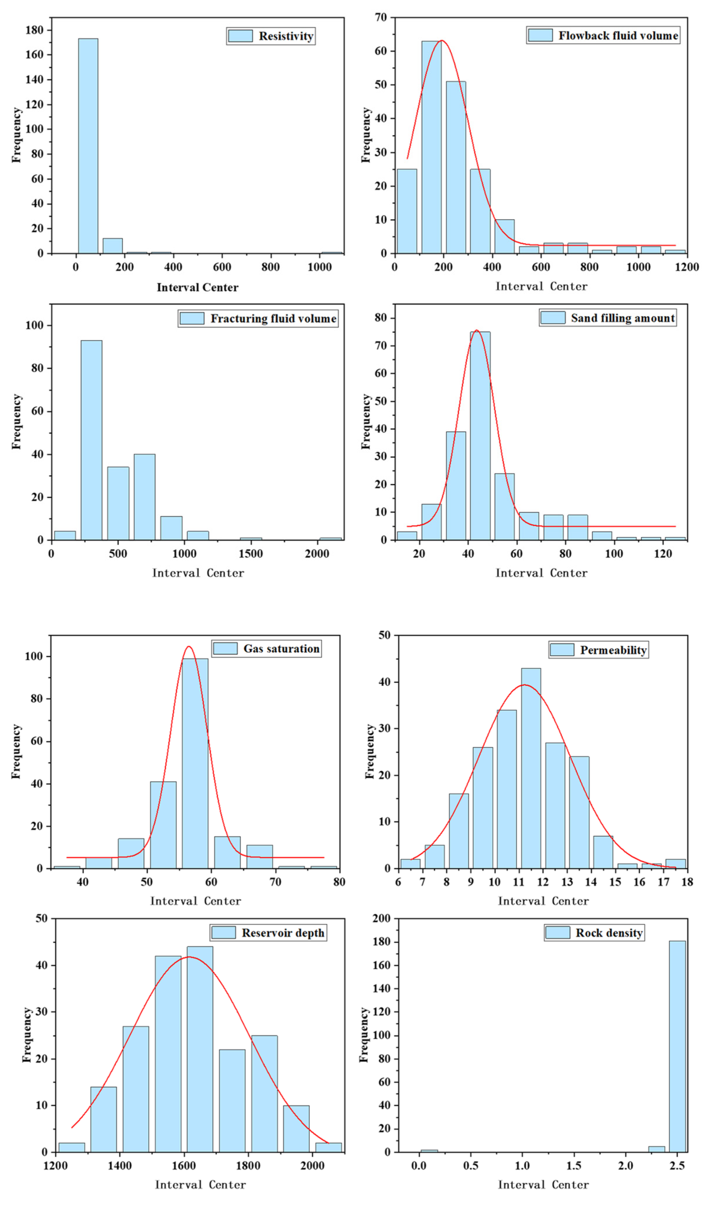
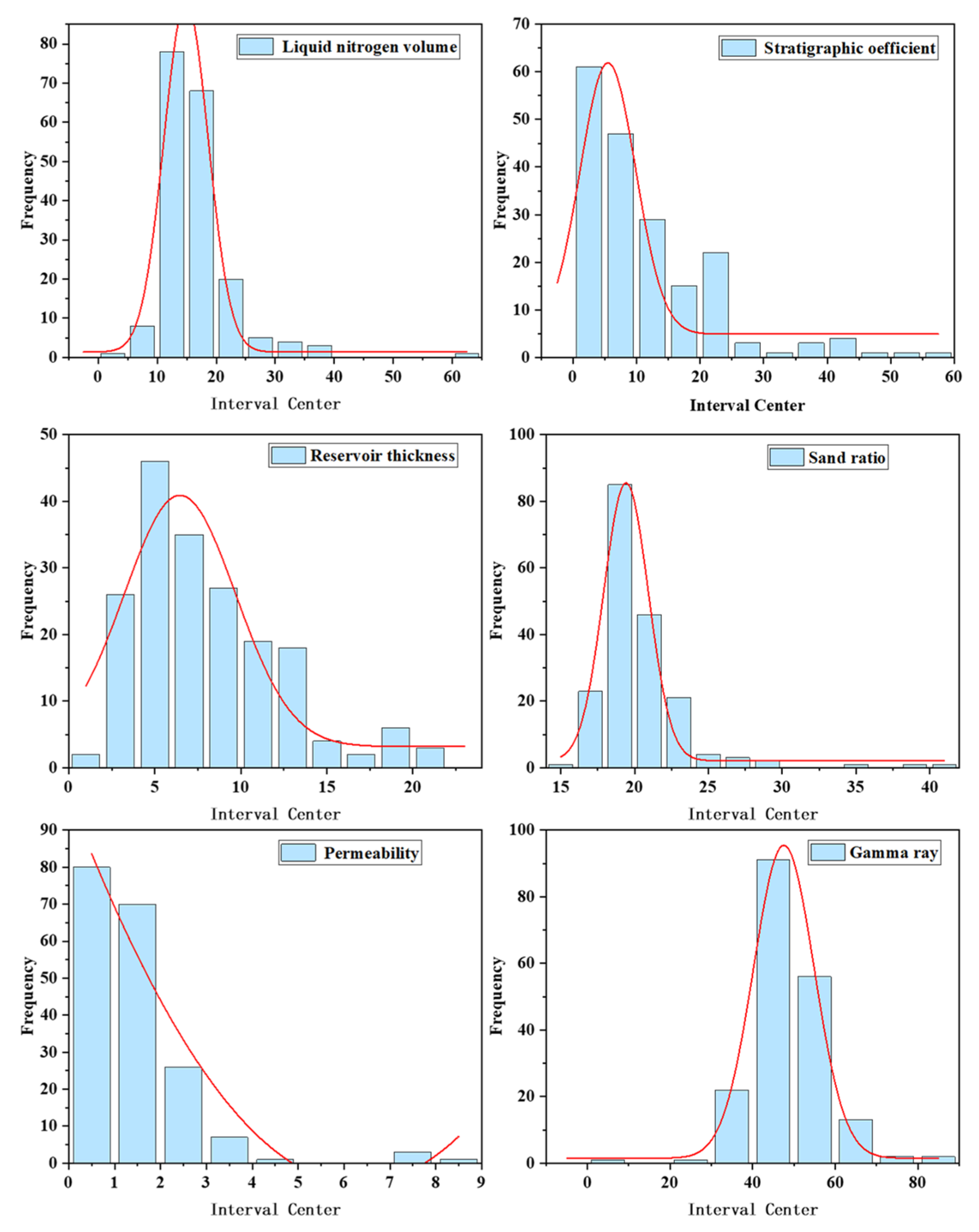
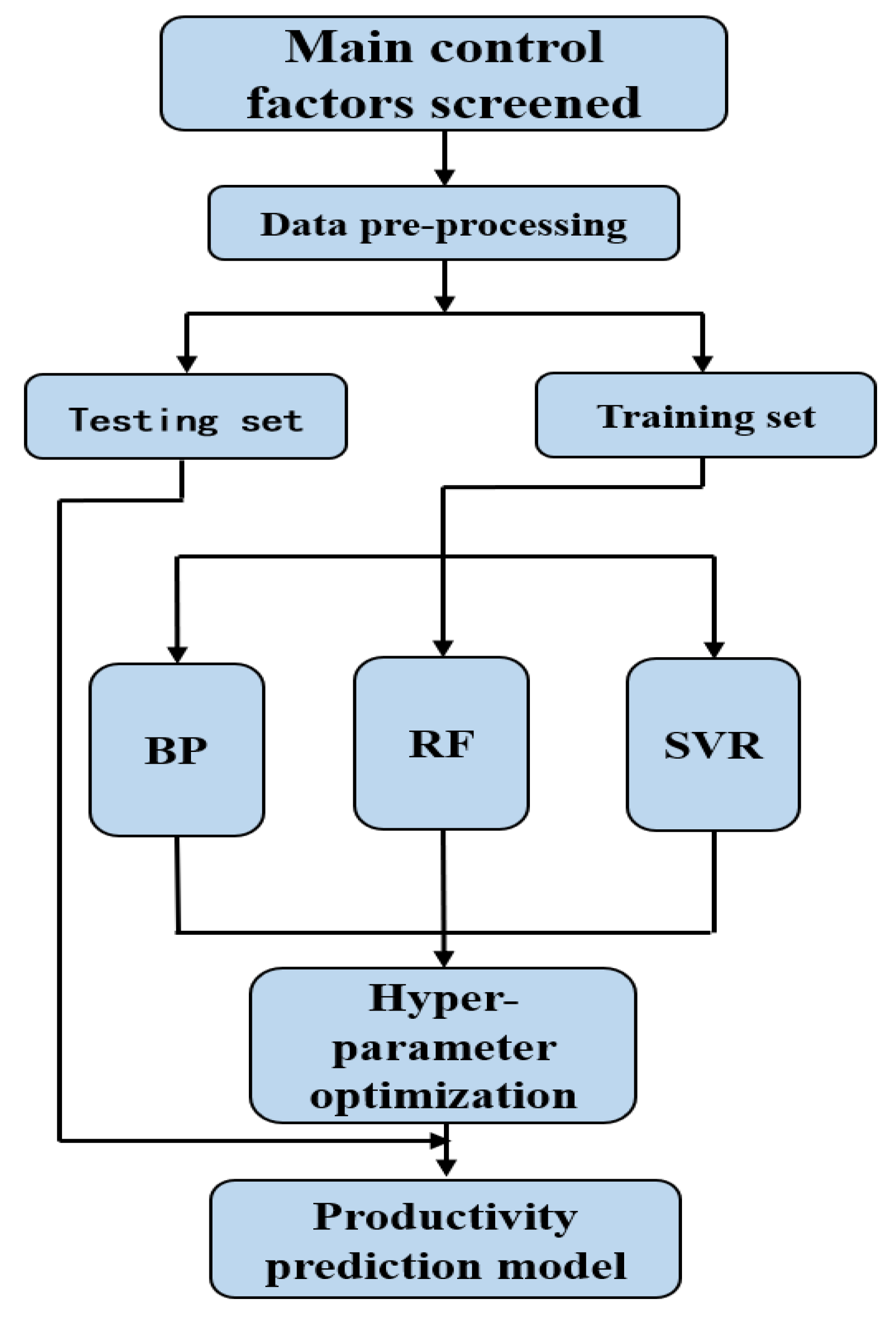
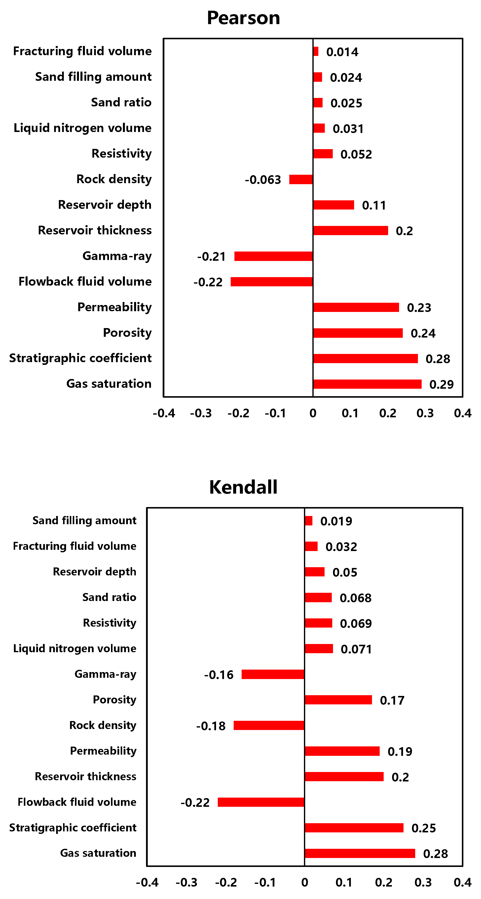
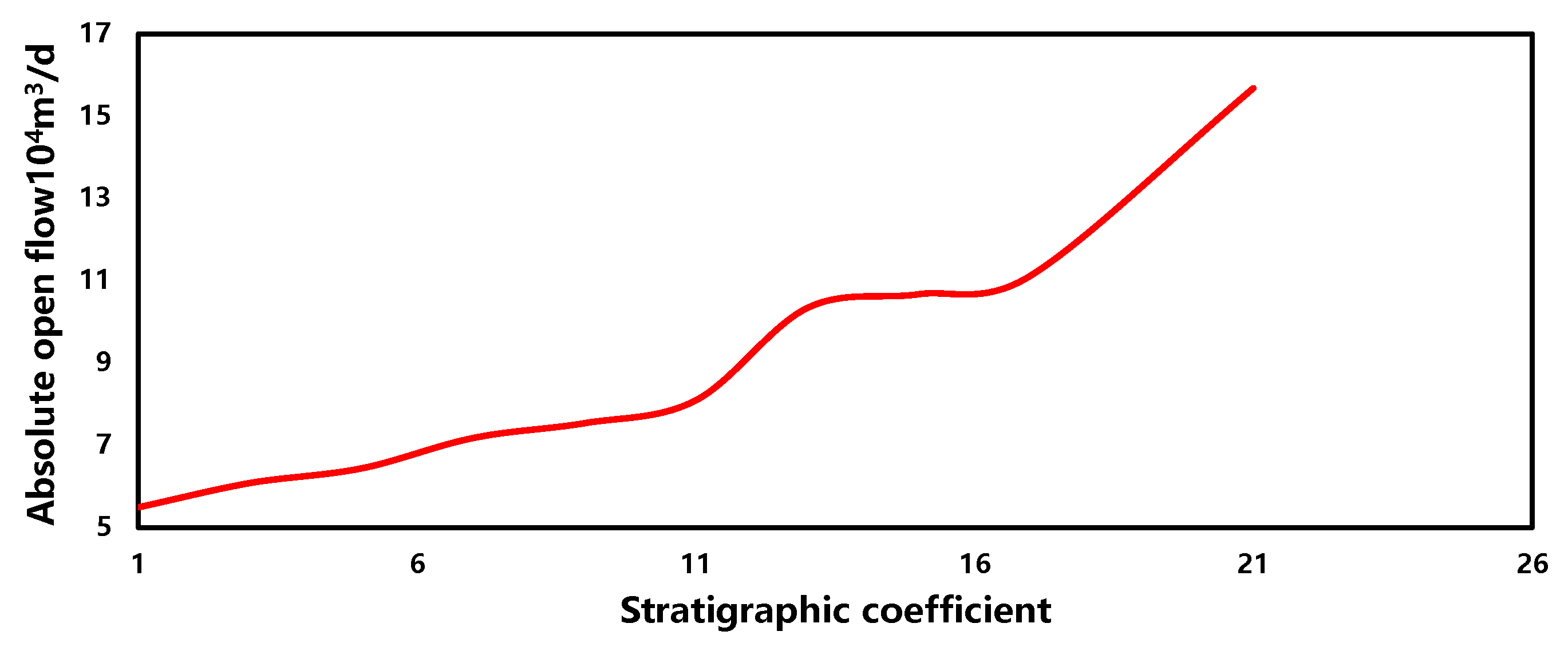
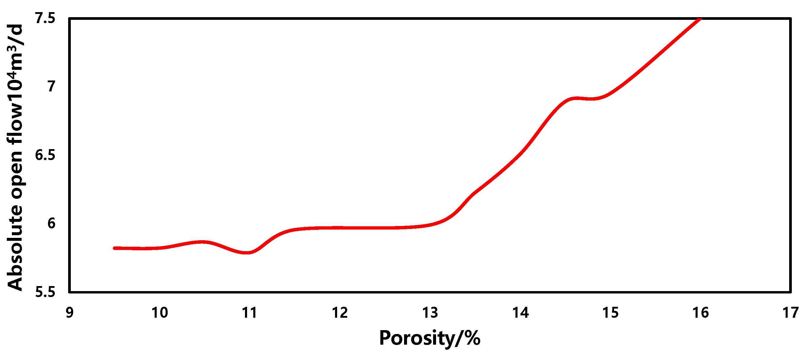
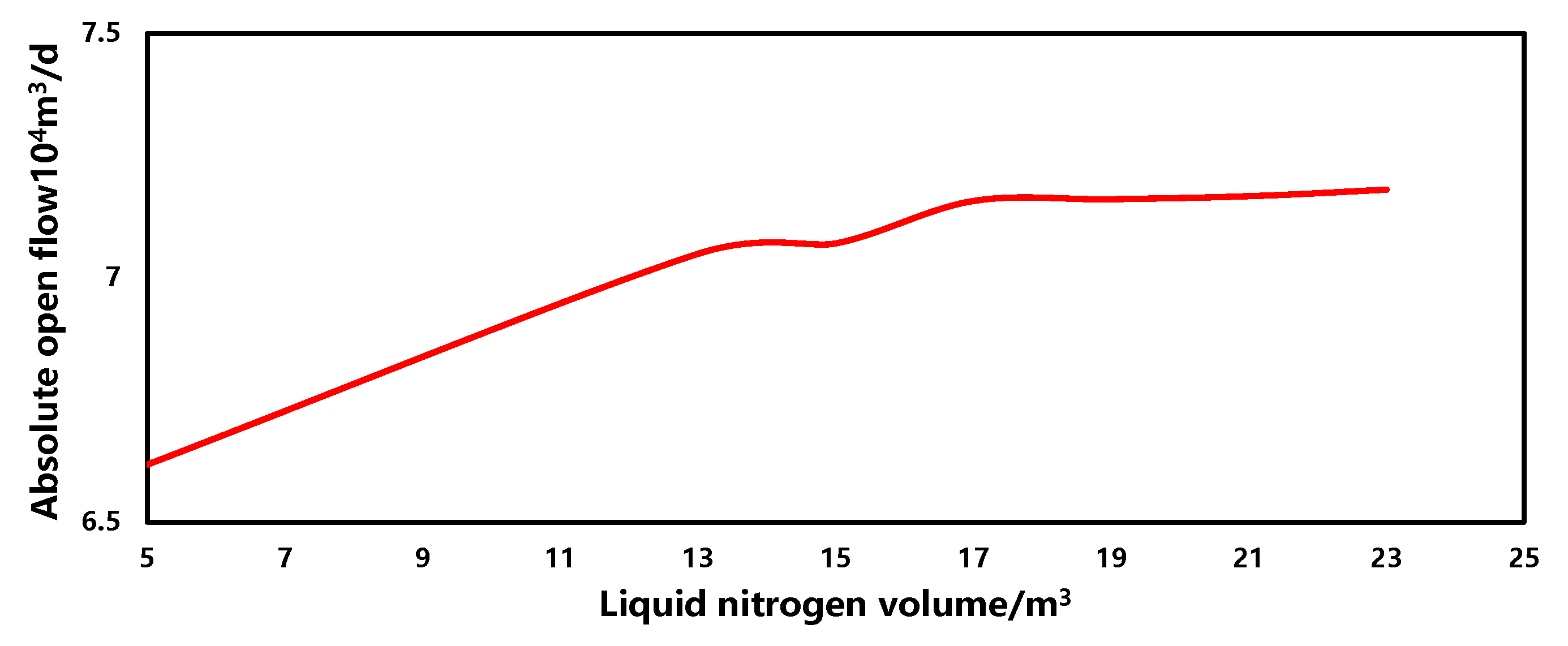
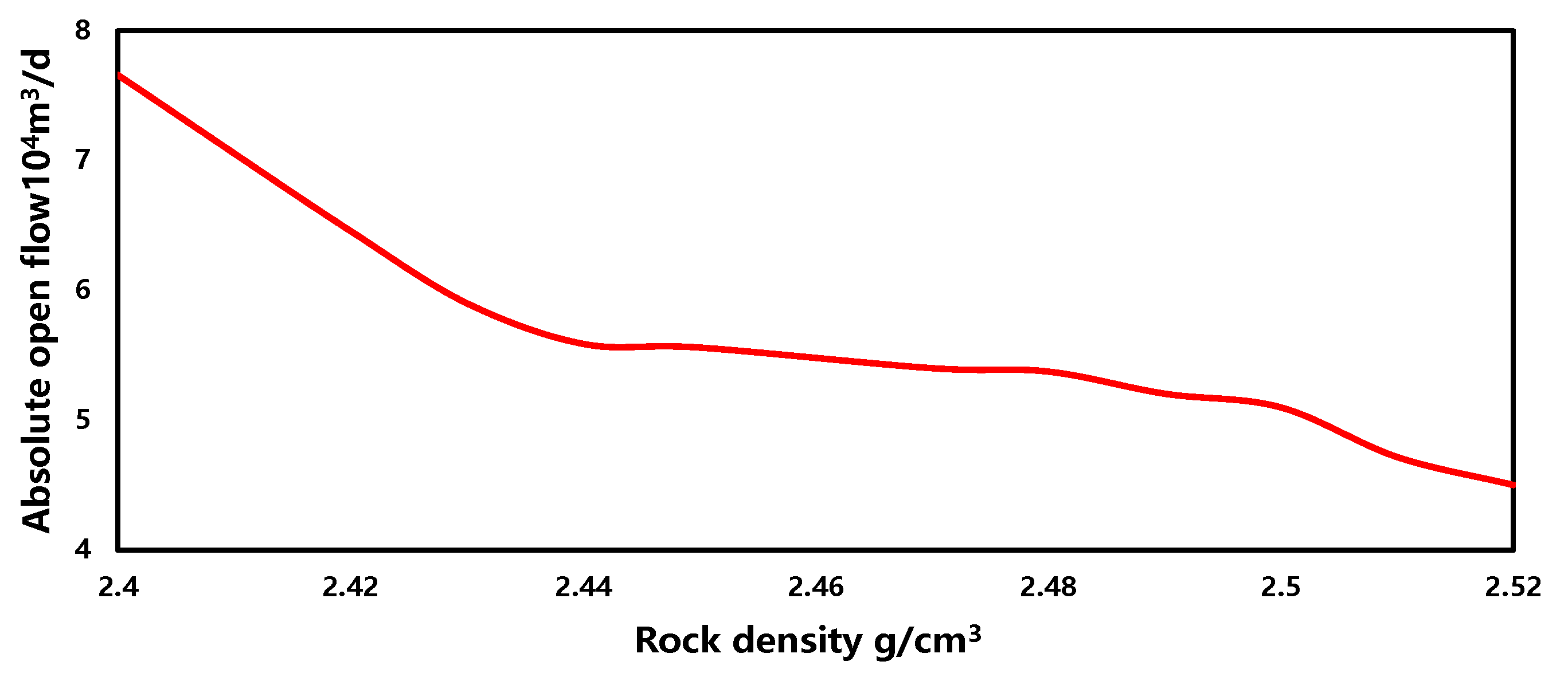
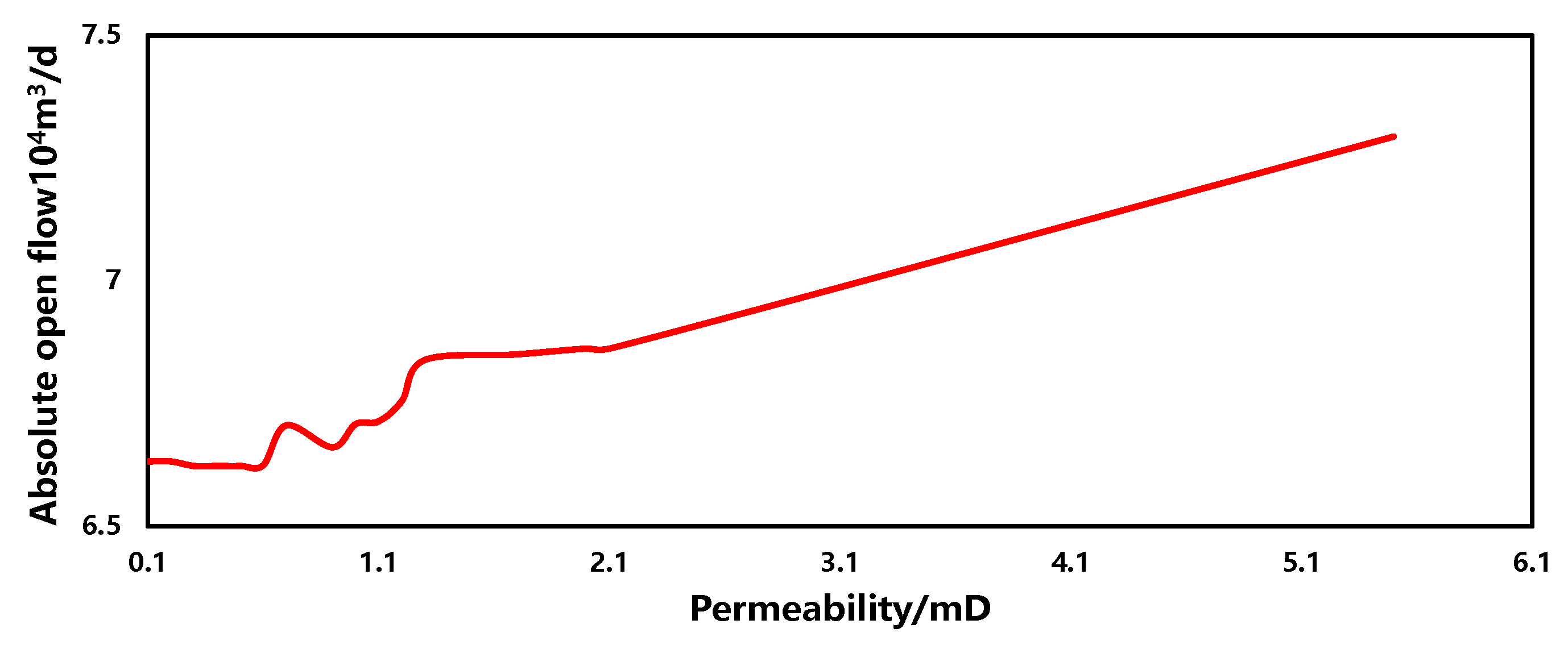
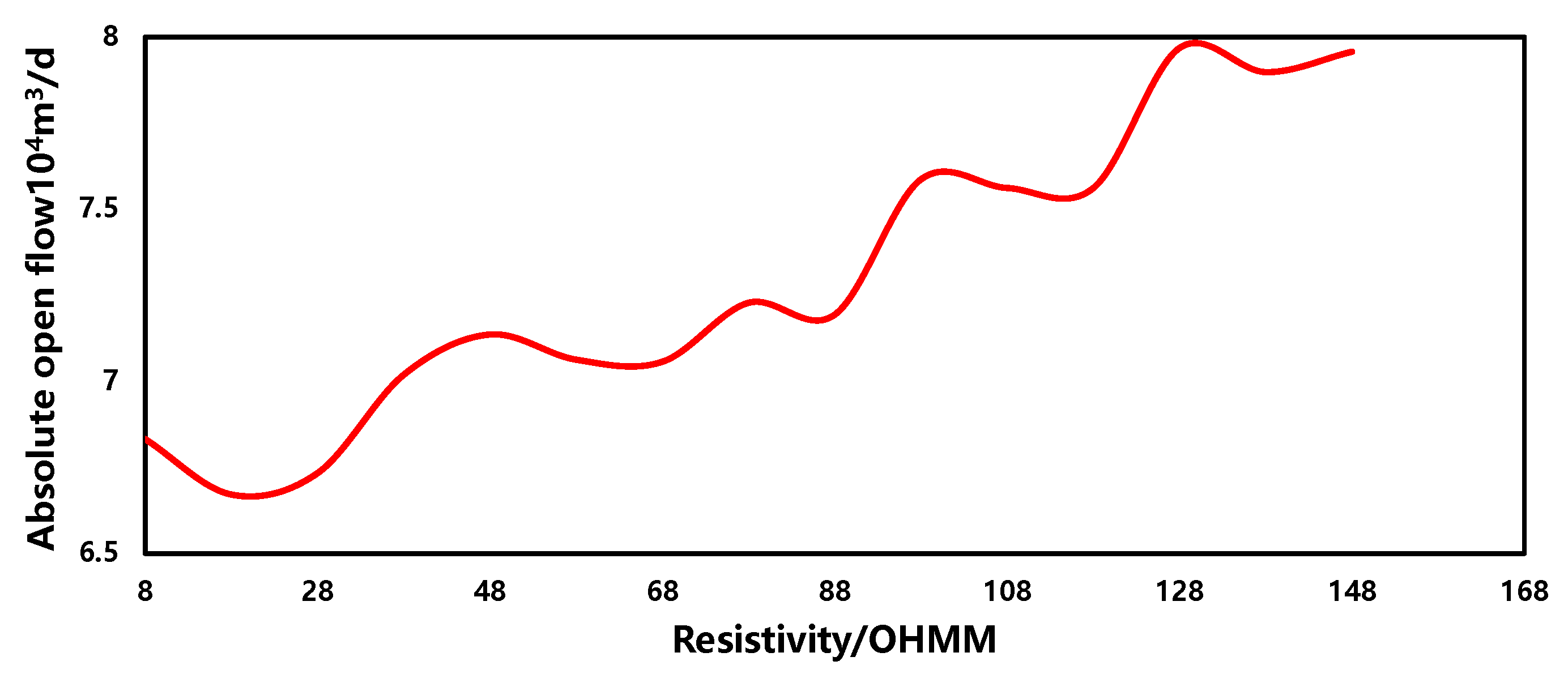
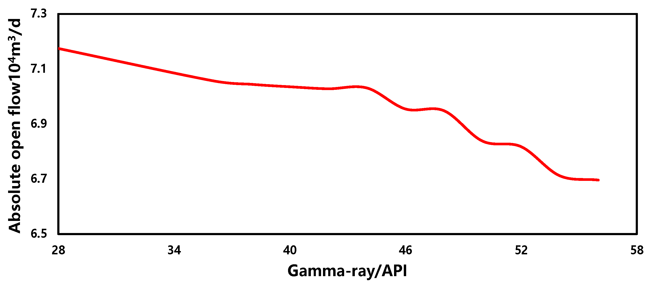
The prediction accuracy of machine learning methods depends on the quantity and quality of data [
18,
19,
20]. Machine learning methods have various adaptabilities and sensitivities to different research data [
21]. Linxing tight gas reservoirs are characterized by high heterogeneity, low pressure, and heterogeneous water saturation. There are nonlinear relationships within the data. Therefore, the selected machine learning models must equip adaptive nonlinear and high-dimensional data computing capabilities. This paper utilizes the BP neural network, random forest regression, and support vector machine algorithm to establish the correlation between the dominant controlling factors and absolute open flow. BP is a well-developed machine learning model that can fit nonlinear data infinitely by increasing the number of hidden layers [
22]. Based on the joint decision-making for multiple decision trees [
23,
24], RF efficiently processes multi-dimensional data and has a strong ability for avoiding overfitting. SVR maps data into high-dimensional space through the kernel function method [
25], significantly improving the efficiency of processing nonlinear data. In addition, this study uses an optimization algorithm to enhance the prediction accuracy of the model. From the field application perspective, the best prediction model for different well types is screened by analyzing the adaptability of the models. The single well recoverable reserves are forecasted by considering the decline curve model. In addition, this study provides a theoretical basis for formulating and revising the development plan of Linxing tight gas reservoirs.
4. Model Application
Due to the highly heterogeneous gas reservoirs, the production systems and fracturing conditions between gas wells are different, resulting in significant differences in the recoverable reserves of gas wells in the Linxing field. Therefore, an effective method is needed to improve the estimation accuracy of EUR for gas wells. Typically, the prediction of single well recoverable reserves uses decline curve analysis combined with historical production data. This method is challenging in regard to determining the initial production for the unexplored area. In this study, a machine learning-based method is proposed for estimating single well recoverable reserve predictions based on geological and fracturing parameters in the early stages of gas well production.
4.1. Decreasing Curve Prediction
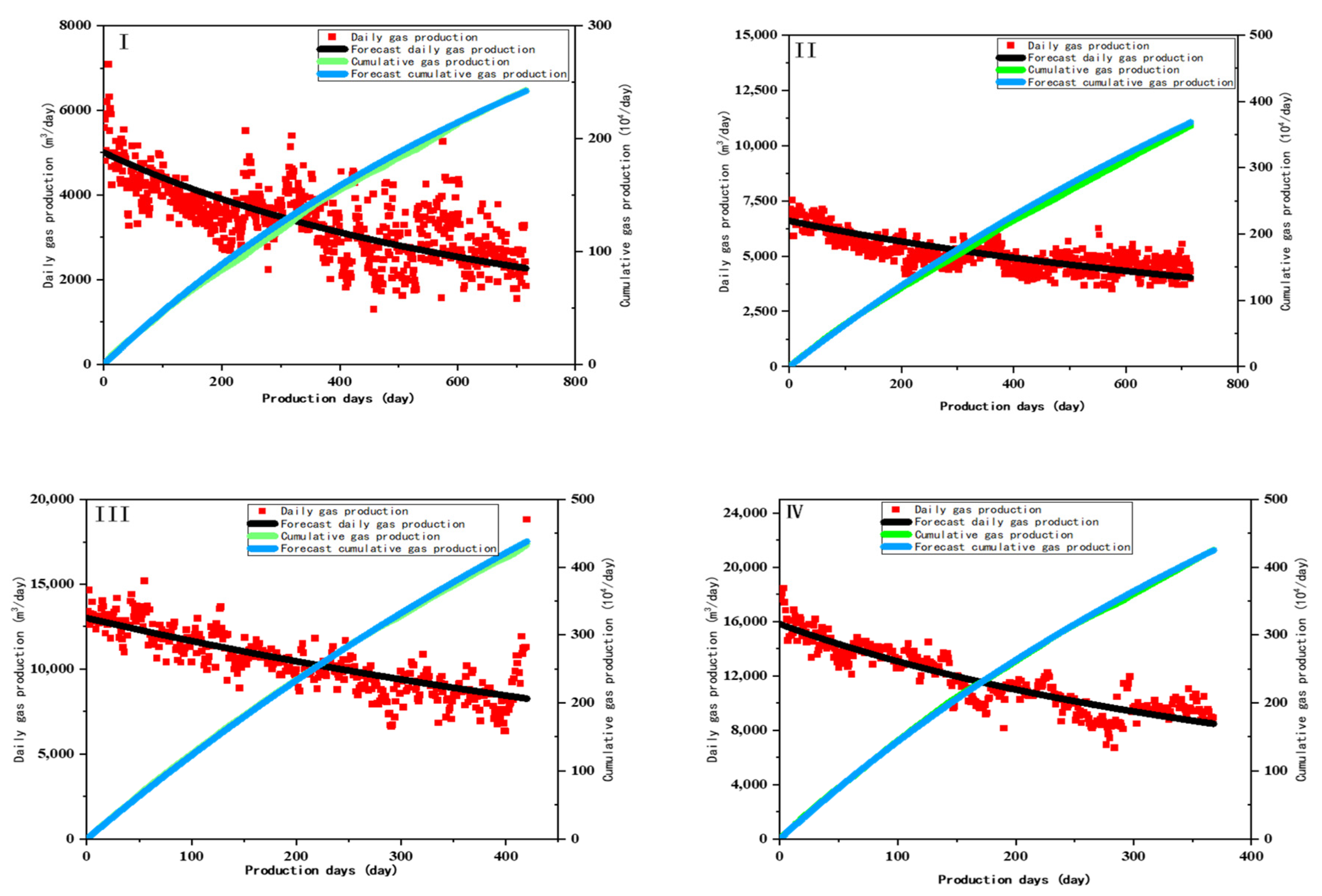
The gas wells in this block of Linxing are mainly characterized by high initial production and short stable production time. Typically, the Arps decline method is employed in the field to predict the EUR of a single well. Decline curve analysis is a classic method for predicting the production decline of oil and gas wells. The best-fitting model is selected based on the historical production data of the field. A characteristic of gas production in this block is a rapid production decline after a short period of constant production (control flow rate) and a stable production state (slow production decline), which generally satisfies the feature of hyperbolic decline. Therefore, the hyperbolic decline model is utilized to fit the gas production in the Linxing gas field and determine the features of gas production in this block.
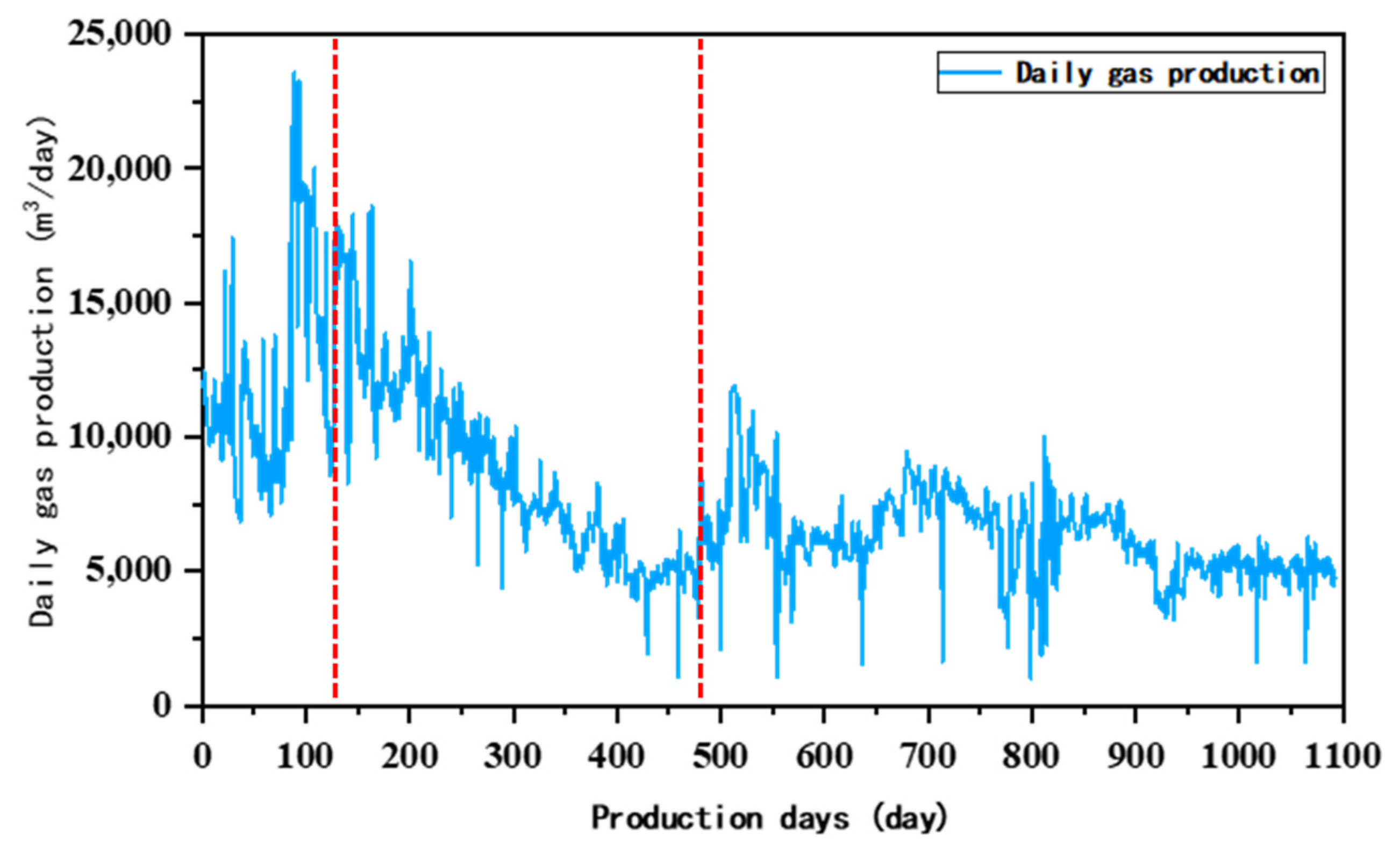
Generally, the production potential for various gas wells is different, and the well type and well productivity can be classified based on absolute open flow rates. Based on the analysis of the decline rate of gas wells in the Linxing reservoirs, the original three types of gas wells are re-classified into four categories according to absolute open flow rate. Among them, the numbers of Type I, II, III, and IV wells are 42, 40, 30, and 15, respectively. The selected gas wells produced gas for more than 12 months and normalized the production during the decline stage. Then, the hyperbolic decline curve is used to fit the production of four types of wells to obtain typical decline curves. The cumulative gas production is used to evaluate the performance of curve fitting, as shown in
Table 6 and
Figure 19. Between the two red lines is the gas well depletion period.
The fitting results of the gas production decline curve are shown in
Figure 20. The production of Type I wells has the most significant fluctuation due to the rapid water breakthrough. In addition, water accumulation occurs in the wellbore in the early testing stage and repeatedly happens during the production stage. Foam drainage operation is a commonly used solution for resolving accumulated water in the wellbore problem, but the operation causes considerable gas production fluctuations.
I well hyperbolic decline fitting formula:
II well hyperbolic decline fitting formula:
III well hyperbolic decline fitting formula:
IV well hyperbolic decline fitting formula:
Type II wells have the smallest decline rate, followed by Type III and Type I wells. Type IV wells have the highest decline rate because the early production of these wells is assigned very high, resulting in insufficient energy supplies and a rapid decline in gas wells. Therefore, the ratio of the average open flow rate of each type of gas well to the initial production of the typical decline curve provides a more reasonable initial co-production basis for the site, as shown in
Table 6.
4.2. RF Model Prediction
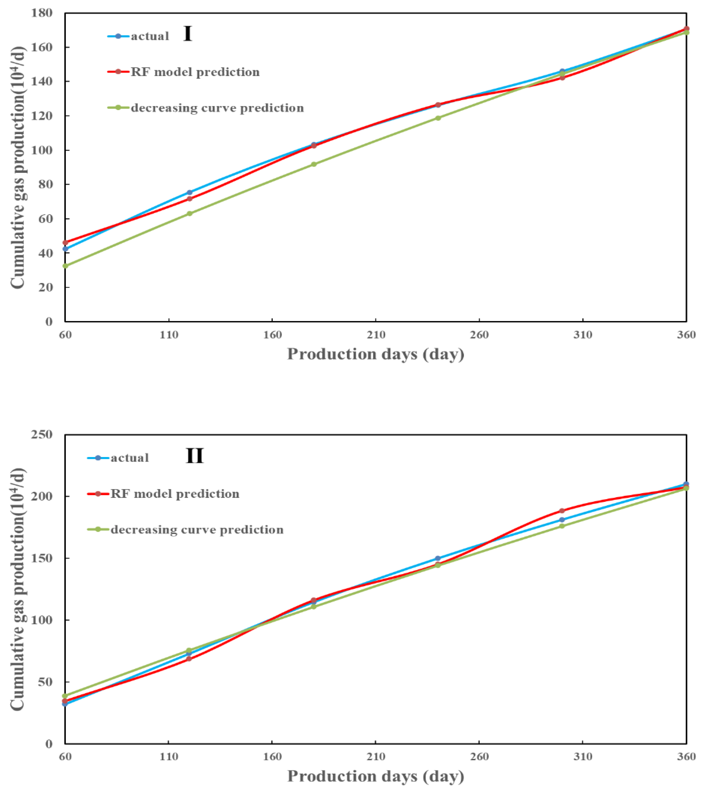
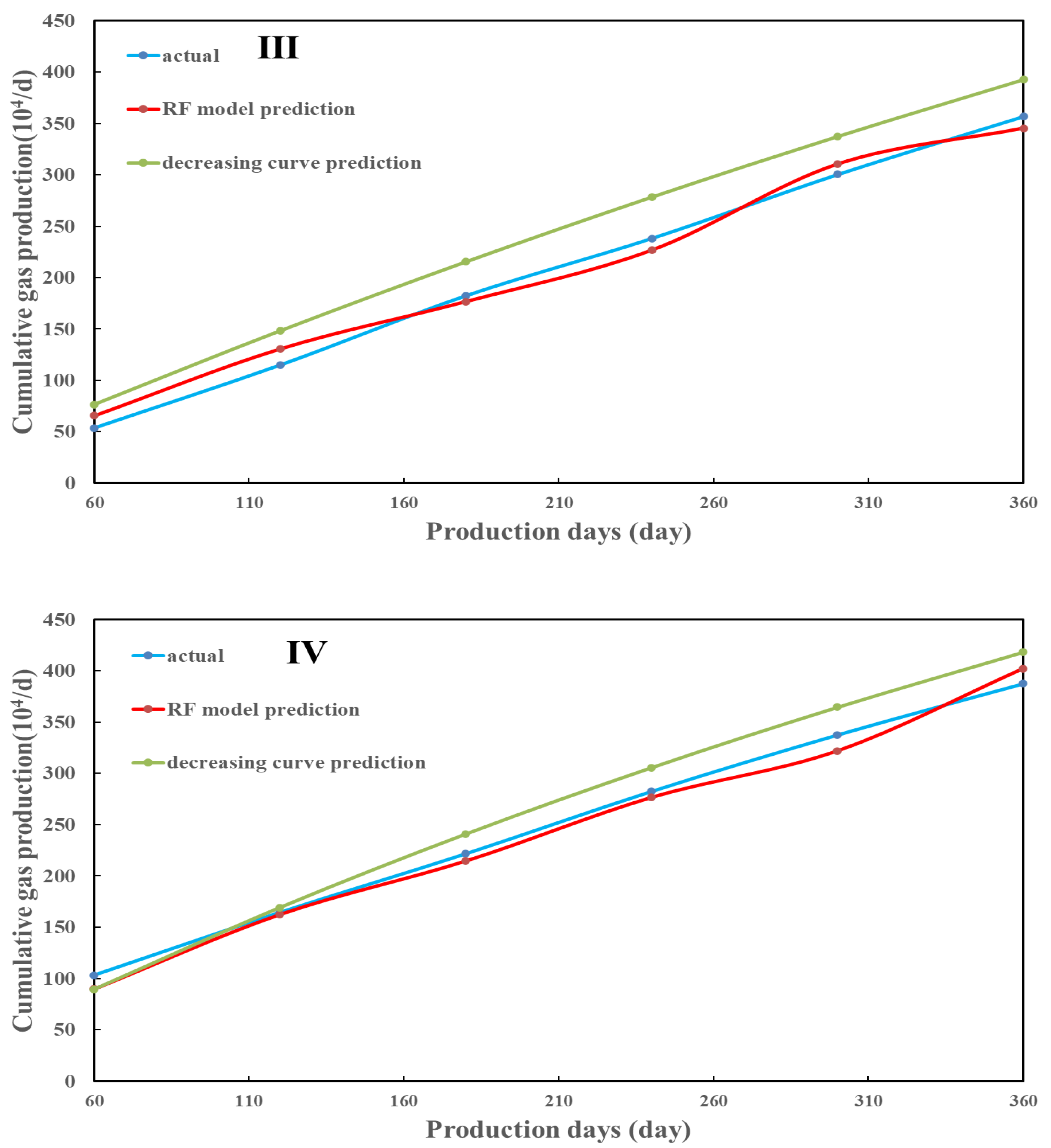
The initial and cumulative production correlation is established using the RF model to predict the cumulative production of the four wells at different stages (with two months as a stage) during the first 12 months. The results were compared with the prediction results of typical decline curves to evaluate the performance of machine learning in production prediction.
Figure 8 shows the predicted 12-month cumulative production errors of Type I wells using the RF model, and the typical decline curve models are 0.07% and 1.12%, respectively. The prediction effect of the RF model is significantly better than that of the typical decline curve model. The errors of Type II wells for the two models are 1.17% and 1.65%, respectively, and the prediction results of the RF model are better agreed with the actual cumulative production trend. For Type III wells, errors are 3.2% and 10.08%, respectively, and the prediction results of RF are more dominant in each stage. The errors of Type IV wells for the two models are 3.8% and 7.9%, and the RF model is more accurate than the decline curve method. Therefore, we conclude that the prediction accuracy of the RF model is better than that of the typical decline curve model, which avoids the influence of the initial production error on the cumulative prediction. During actual gas production, various operations are often conducted in the field, resulting in output fluctuations during production. The decline curve cannot eliminate this difference, significantly impacting production forecasting. As shown in
Figure 21, the prediction results of the machine learning model are more in line with the actual production.
4.3. EUR Prediction
The medium and high-producing wells (named Well
−1, Well
−3, and Well
−5) are randomly selected from the database to predict 20-year EUR using two methods. As shown in
Table 7, the absolute open flow rate of the gas well indicates the production potential of the well. Combined with the typical decline curve of different types of wells, the EUR of a single well can be predicted. The forecasted 20-year EUR for Well
−1, Well
−3, and Well
−6 is 958.8 × 10
4 m
3, 1819.9 × 10
4 m
3, and 4109.8 × 10
4 m
3, respectively. Compared with the prediction results of OFM software (2014V2), the differences for the three wells are 9.9%, 13.7%, and 6.5%, respectively, and the differences are all within the acceptable range.
Oil Field Management (OFM) software predicts the recoverable reserves of a single well based on the historical production of wells. The proposed machine learning-based model can complete the prediction at the early stage of geological analysis. The method uses machine learning models to reveal the correlation between productivity with geological and fracturing parameters, as well as to predict the absolute open flow rate of gas wells. Combined with the typical decline curve, the model can predict the recoverable reserves of a single well, which provides an effective method for determining the productivity potential of gas wells and planning new wells. In the process of economical cost, the overall work efficiency is improved. As EUR prediction is completed before the production period, it provides insight into the surface facility and piping design to improve the project’s economics.
5. Conclusions
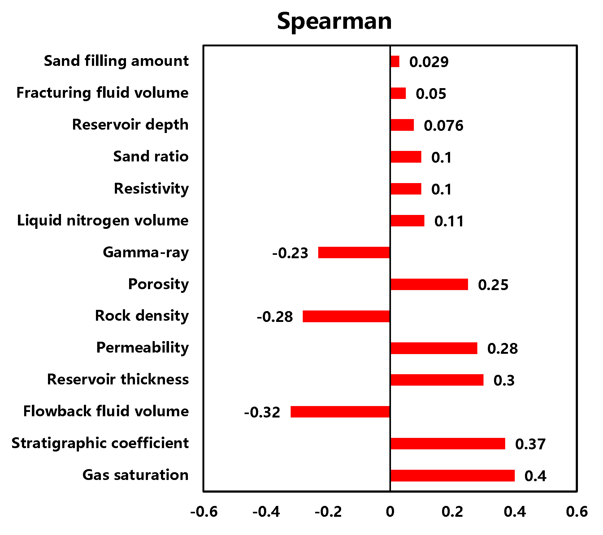
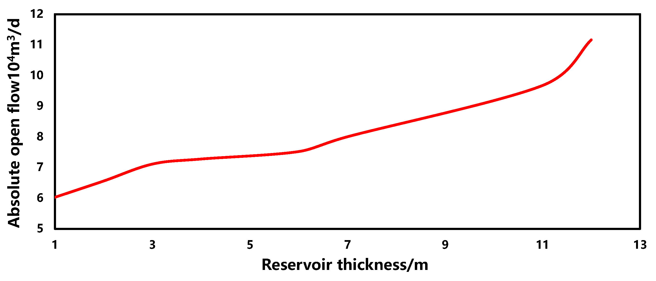
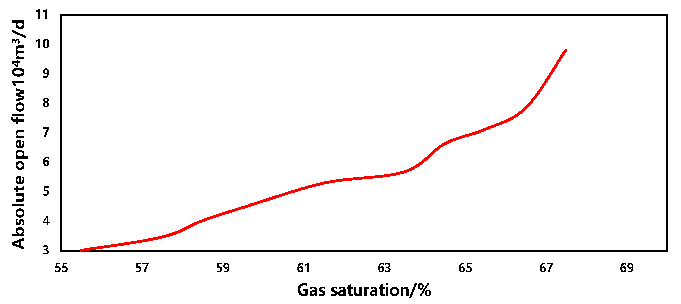
(1) The statistical analysis method can quickly determine the dominant controlling factors of well productivity and provide a quantitative evaluation. This study analyzes the performance of 10 parameters, including gas saturation, reservoir thickness, etc., on gas well productivity in this block. The results indicate that geological factors play a more significant role than fracturing factors in well productivity prediction.
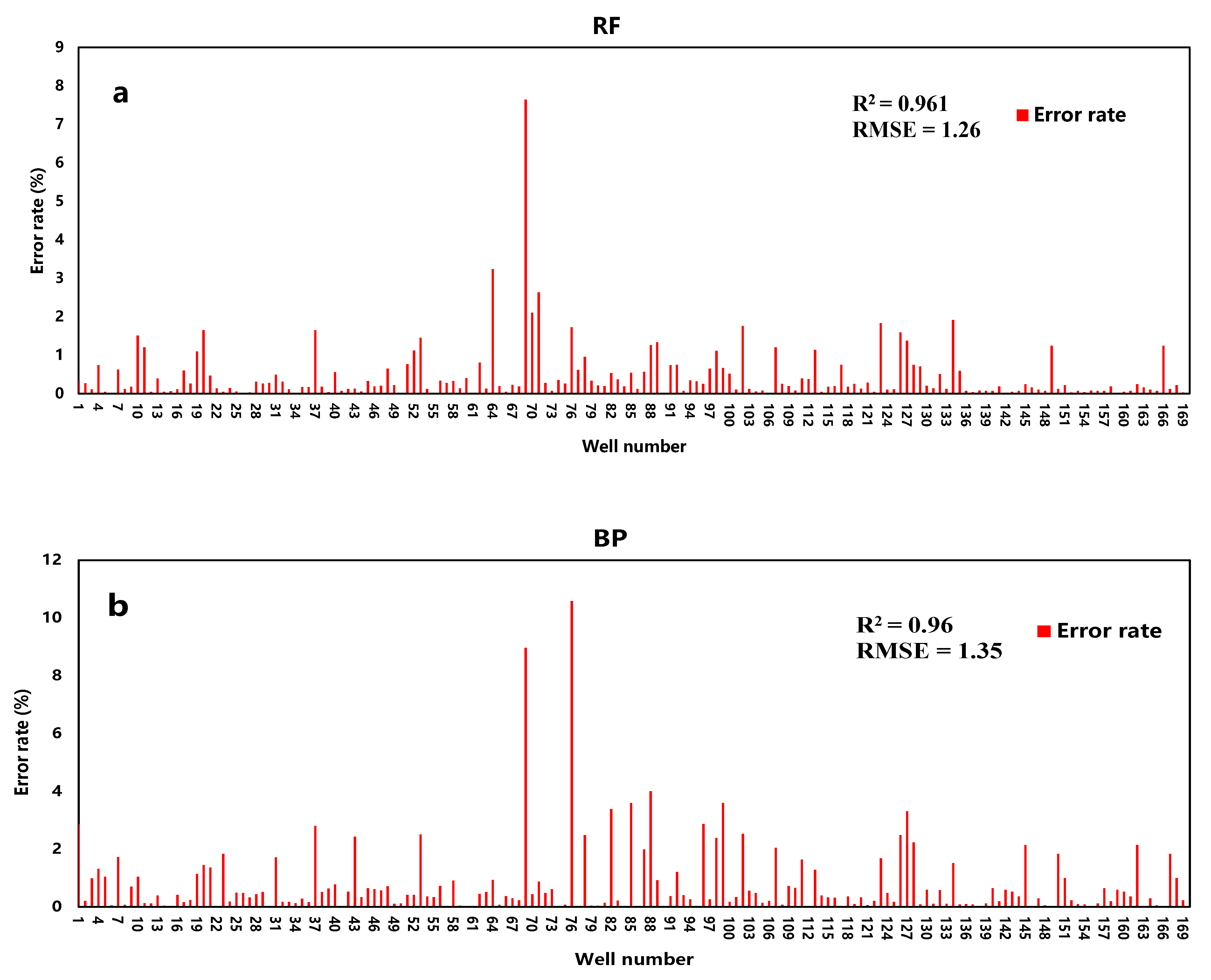
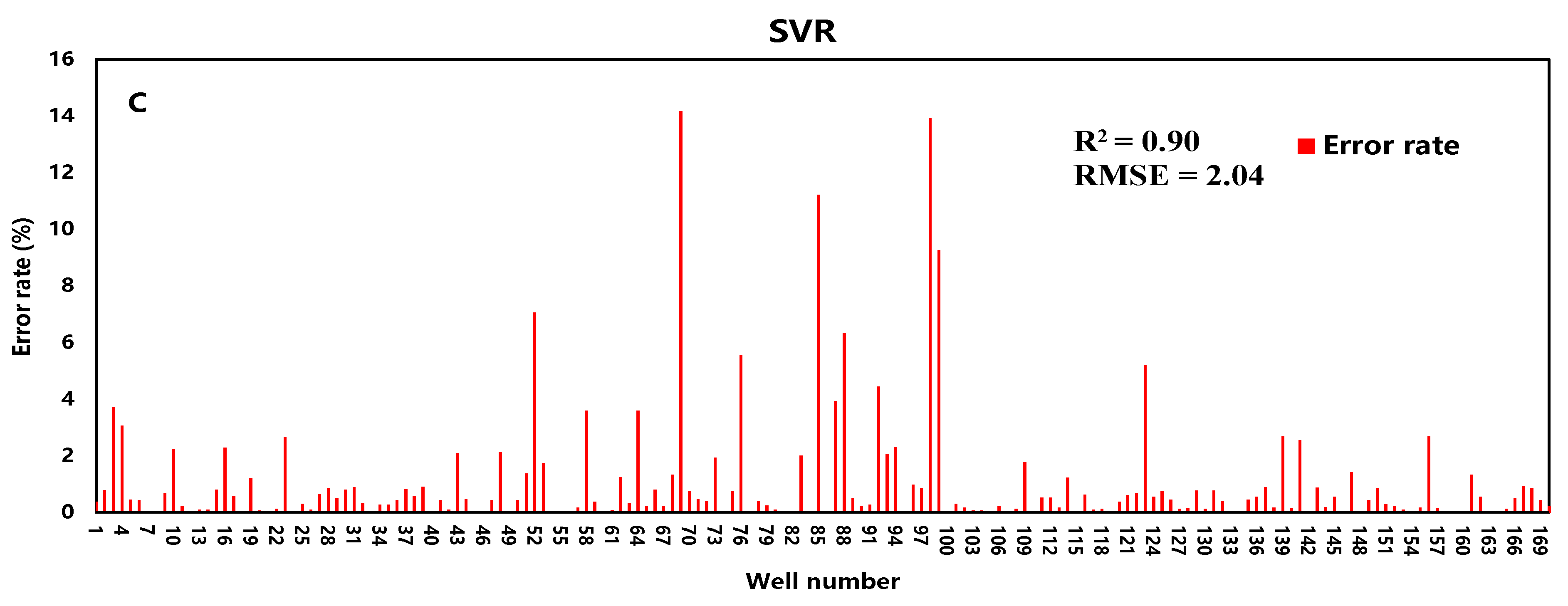
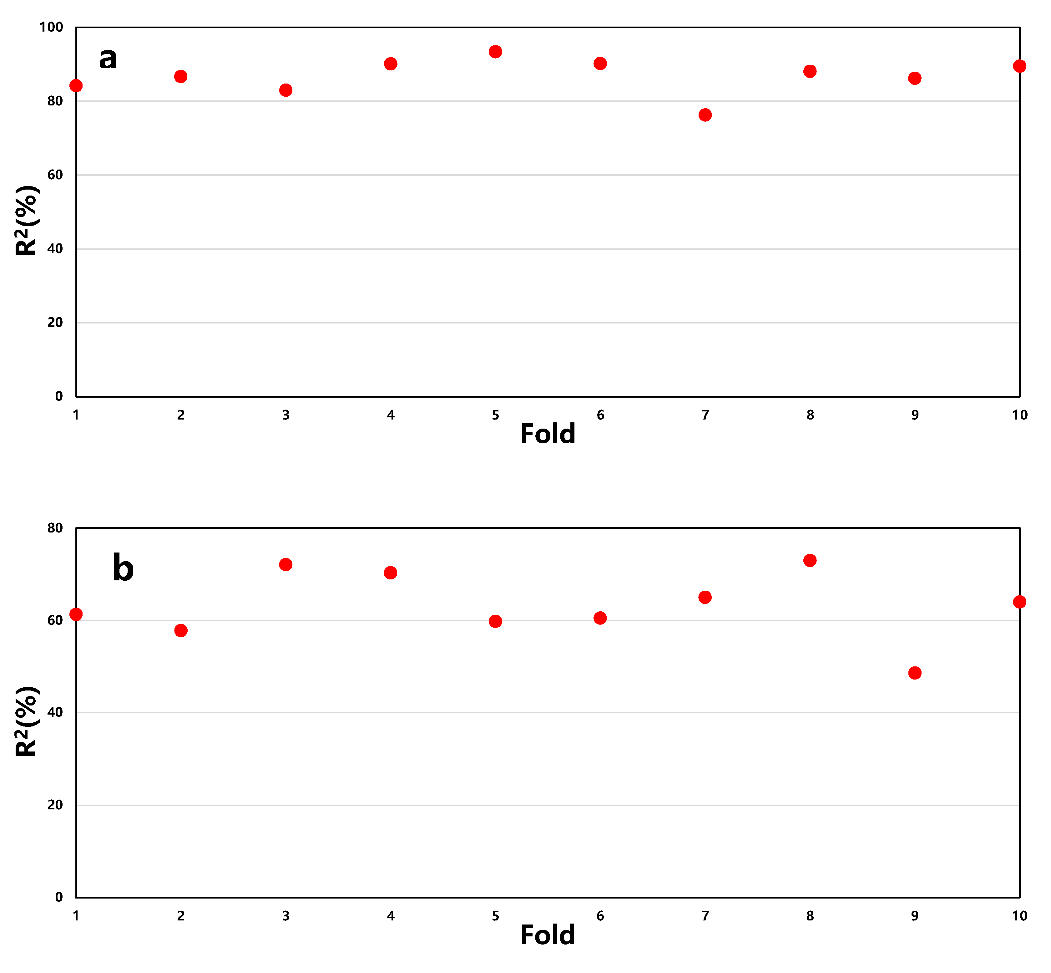
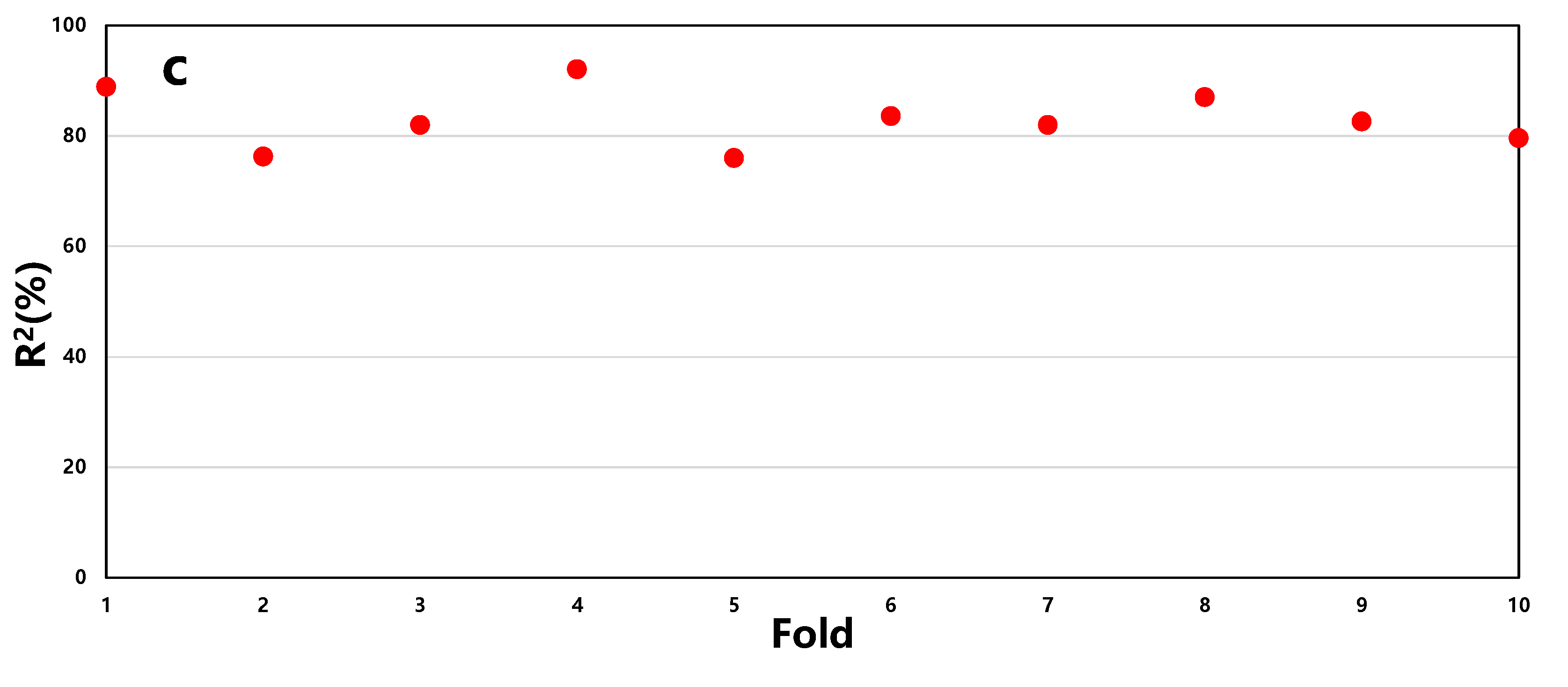
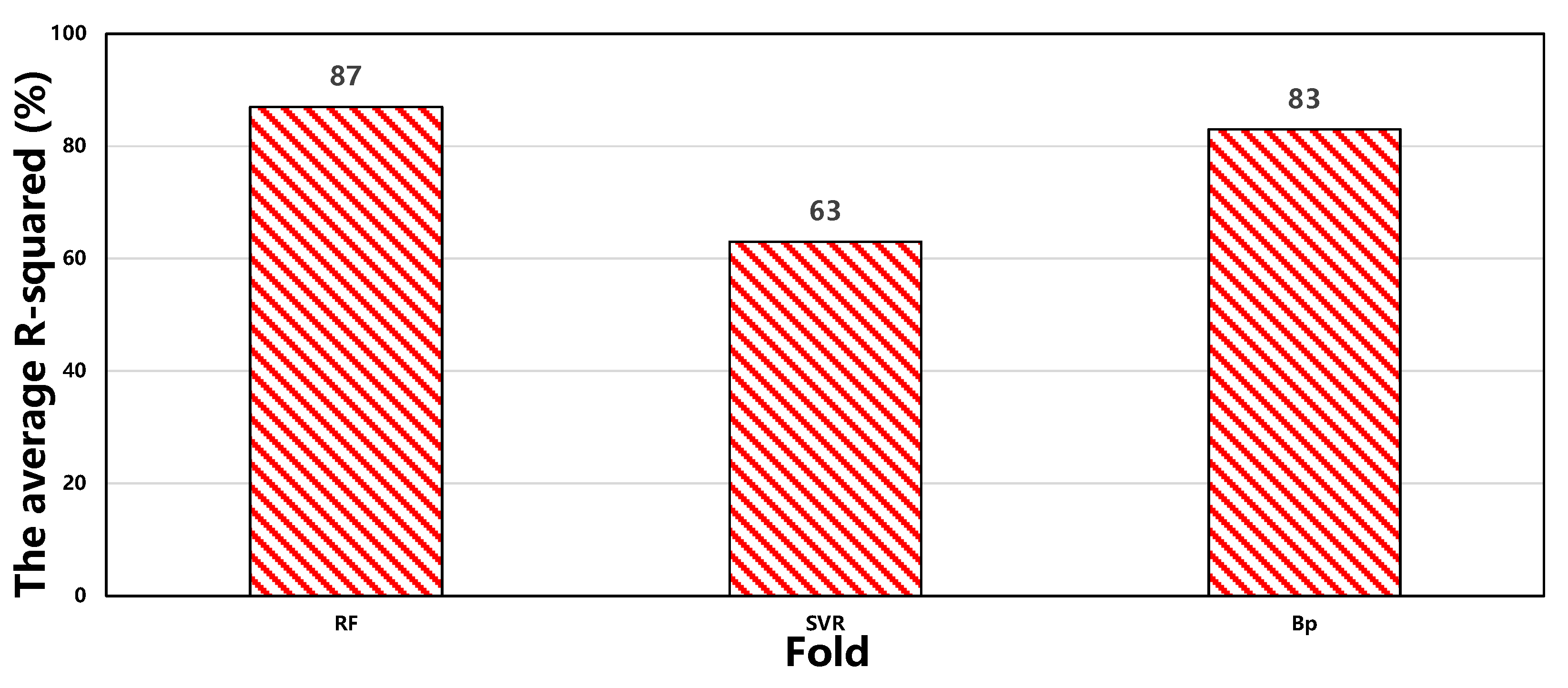
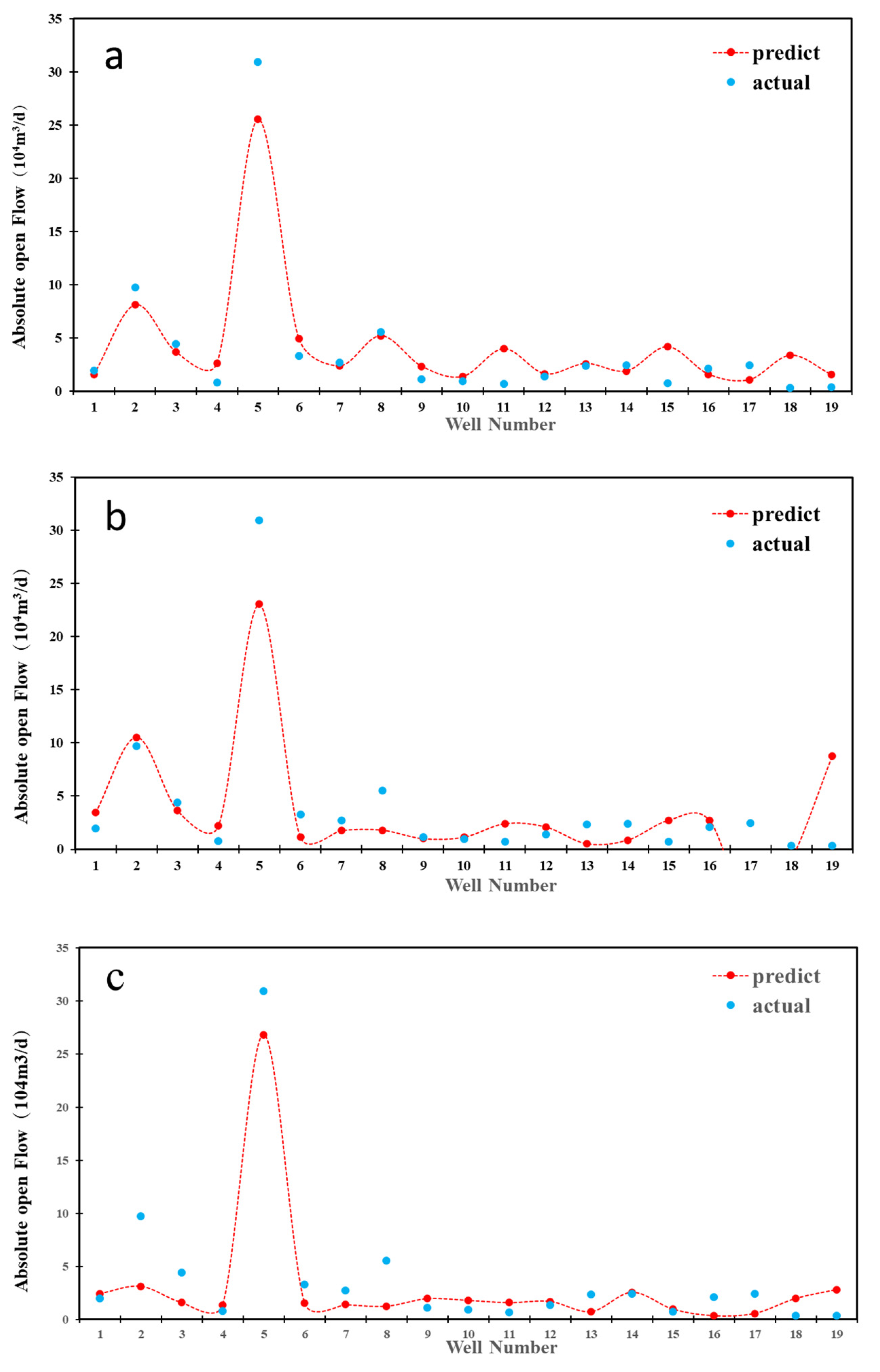
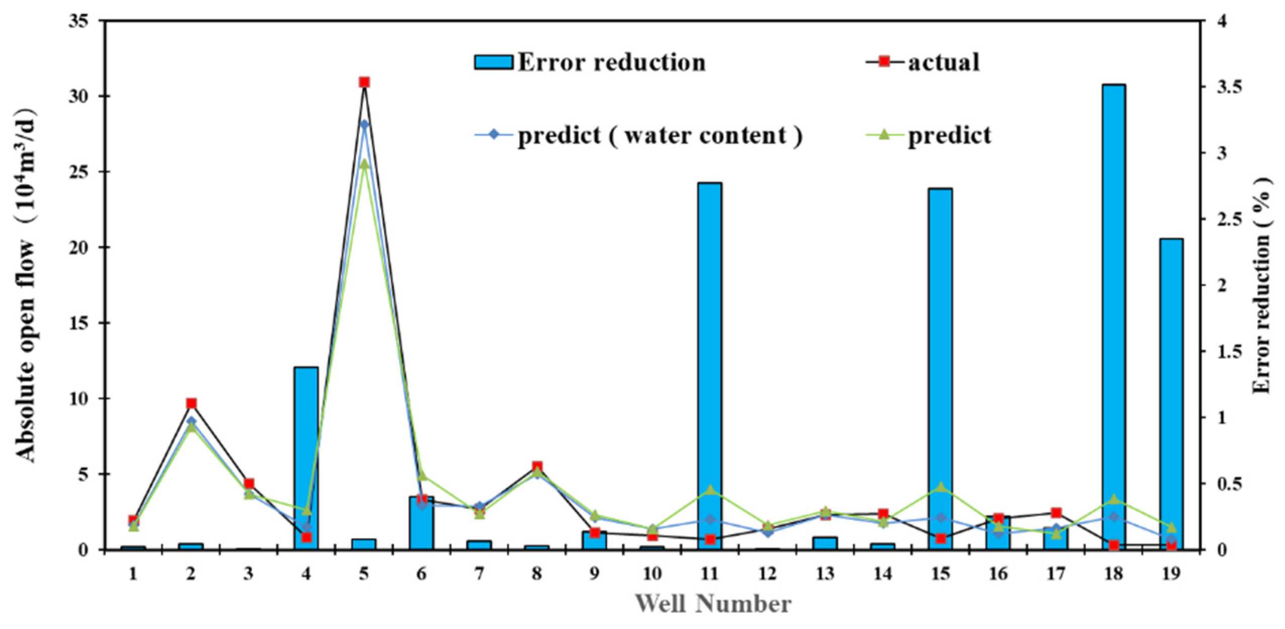
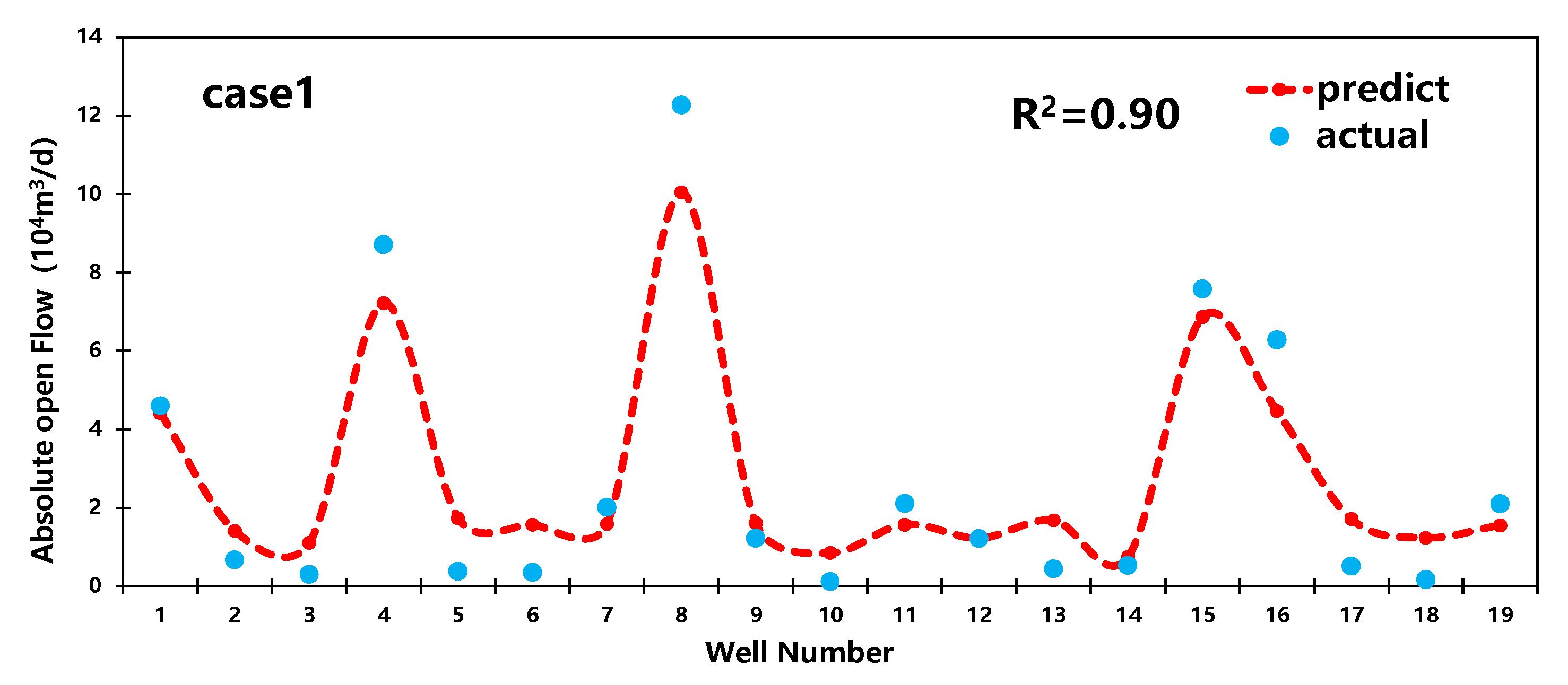
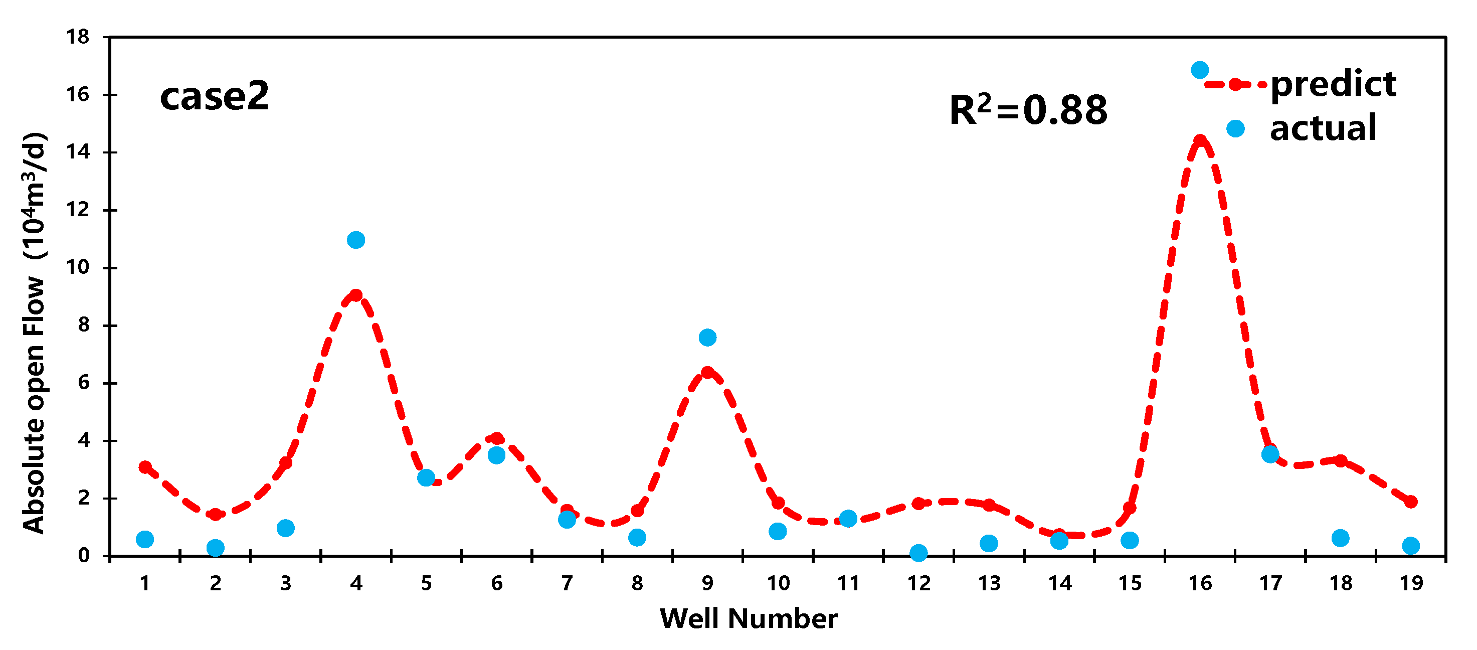
(2) The RF model can accurately predict the absolute open flow of gas wells and distinguish the type of gas wells. Based on machine learning evaluation, the RF prediction model with an RMSE of 3.98 and R2 of 0.91 has the highest prediction accuracy, followed by the BP. The SVR model has the largest prediction error. From the practical application, the RF model entirely (up to 100%) recognizes the medium- and high-production wells. Therefore, the RF model is recommended for employment in productivity prediction in the Linxing gas reservoirs.
(3) The research shows that the deviation of the initial production leads to inaccurate prediction results regarding the typical decline curve. It is challenging for the typical decline curve to capture the character of actual production for the wells that conducted multiple operations. The 12-month cumulative production forecasting of the four wells using the RF model is more accurate than the typical decline curve model, verifying the applicability of machine learning in production prediction.


