MLD Modeling and MPC-Based Energy Management Strategy for Hydrogen Fuel Cell/Supercapacitor Hybrid Electric Vehicles

Abstract

Energy management strategies for hydrogen fuel cell hybrid electric vehicles (FCHEVs) are a key factor in achieving real-time vehicle energy optimization control, vehicle driving economy, and fuel cell durability. In this paper, for an FCHEV equipped with a fuel cell and supercapacitor, the quantitative information, logic rules, and operational constraints are transformed into linear integer inequalities according to its different operating modes, and the Hysdel language is used to establish its mixed logic dynamic model (MLD). Then, the energy management strategy based on model predictive control (MPC) is developed using the MLD model as the prediction model and the equivalent hydrogen consumption and the performance degradation of the fuel cell as the optimization performance indexes. Finally, under the World Light Vehicle Test Cycle, a joint simulation was carried out with Advisor and Simulink to verify the proposed strategy’s superiority by comparing it with the power following control strategy (PFCS) and the compound fuzzy control strategy (CFCS). The results show that the strategy not only ensures real-time FCHEV energy control, but also reduces hydrogen consumption by 10.98% and 1.98% and the number of start/stop times of a fuel cell by six and four, compared to PFCS and CFCS, respectively, which improves the economy of the whole vehicle as well as the durability of the fuel cell.

1. Introduction

According to the International Energy Agency (IEA) [1], the world’s vehicle ownership was about 1.5 billion in 2020, and despite the impact of the COVID-19 epidemic, transportation still accounted for over 53% of global oil consumption and around 37% of global CO₂ emissions. The use of new energy is a solution to improve the environment and reduce dependence on fossil fuels, and the unique advantages of low-carbon hydrogen energy are promising and irreplaceable for a wide range of applications in industry and transportation [1]. Hybrid vehicles with hydrogen fuel cells (FCs) as the main energy source are gradually developing in the field of new energy vehicles. Fuel cell hybrid electric vehicles (FCHEVs) equipped with FCs and supercapacitors (SCs) can improve the economy of the whole vehicle by reasonably distributing the power of the two energy sources, so that the comprehensive performance of the whole power system can reach the best state [2].

Based on different control methods, energy management strategies for FCHEVs are generally classified into three main categories: rule-based, optimization-based, and learning-based [3]. Rule-based strategies are further categorized into deterministic rule-based [4] and fuzzy rule-based [5], which do not require precise modeling and are simple and easy to apply in practice, but have difficulty in achieving the optimal effect, and whose parameters are greatly affected by the vehicle driving conditions [3]. Optimization-based strategies mainly include global optimization and real-time optimization. Global optimization strategies, such as linear programming (LP), dynamic programming (DP), etc., require prior knowledge of the full driving condition information and the establishment of accurate mathematical models [6], need more complicated optimization calculation, and are difficult to be applied in practice and are mostly used for theoretical analysis. Learning-based strategies include reinforcement learning, neural networks, support vector machines, etc. The main advantage is that they are based on data and do not require modeling, but they require a lot of time to build libraries and complex artificial intelligence knowledge [7]. The following discussion focuses on optimization-based strategies.

Real-time optimization strategies include Pontryagin’s Minimal Principle (PMP), model predictive control (MPC), etc. As a constrained optimization method, PMP requires the introduction of Lagrange multiplier vectors and predicted driving condition information during the optimization calculation [8,9,10,11], and real-time optimization can only be achieved through careful design. MPC [12,13,14,15,16] has gained widespread attention for its superiority in implementing real-time optimal control by transforming global optimization within the entire driving conditions into local optimization within the prediction time domain [17,18,19,20,21]. In energy optimization control based on MPC for the full cell hybrid power system (FCHPS), earlier research was based on dynamic matrix-based MPC control [13], and then, with the goal of improving energy economy, scholars carried out research on single-layer MPC control with an FC + SC structure [14], FC + battery (BA) structure, and FC + BA + SC structure [15,16]. However, the conventional single-layer MPC has difficulty meeting the growing dynamic performance of vehicles as well as multi-objective requirements, and its multi-parameter optimization computation still requires a very large amount of power, so two layers of MPC, the economic optimization layer and the optimization control layer, are used to collaborate and share the task [17]. This type of MPC has the problems of complicating the whole control strategy, how to coordinate among multiple MPCs, and how to guarantee the control performance. In order to solve the multi-objective optimization and real-time problems, the fusion of MPC with other control algorithms is used, such as incorporating fuzzy C-mean clustering combined with a Markov chain [18], and an online learning Markov chain [19] that can improve the prediction speed. However, the questions of how to further reduce nonlinear optimization calculations and how to ensure the optimality and robustness of the control still warrant continuous research. On the other hand, most of the research has been conducted by establishing exact mathematical models, fuzzy prediction models [20], and neural network models [21] as the prediction models of MPC. However, the FCHPS is a hybrid system which includes both continuous dynamic variables and discrete logic variables, and there is constant alternation between the two kinds of variables [14,22]. So, establishing a mixed logic dynamic model (MLD) as the prediction model helps with the MPC-based energy optimization control.

There are two main types of modeling methods for hybrid systems, “aggregation” and “extension” [23]. The so-called “aggregation” method is to divide the interval for the discrete event problem in the system to represent the continuous state. This method is commonly modeled by hybrid Petri net models [24] and hybrid automata models [25]. The “extension” method is mainly based on the MLD and the Piecewise Affine models (PWA). Scholars have tried to apply MLD modeling methods to vehicle engineering, such as through intelligent vehicle longitudinal dynamics [26], yaw stability control of distributed drive electric vehicles [27], and energy management of hybrid electric vehicles [28], but the literature review shows that there is a lack of research on the application of FCHEVs, and further research is needed.

Based on the above analysis of a typical hybrid system for FCHEVs, this paper proposes to establish its MLD model as a prediction model and model predictive energy management strategy for FCHEVs. The mixed-integer linear programming algorithm is applied to achieve the optimization using a minimum of 100 km hydrogen consumption and FC performance degradation as the optimization objectives.

The remainder of this paper is structured as follows. In Section 2, the configuration of the FCHPS and the components are modeled. How to build the MLD model for the FCHPS is discussed in detail in Section 3. A detailed introduction to the energy management strategy based on MLD-MPC is elaborated on in Section 4. In Section 5, the simulation validation is carried out. The performance of the proposed strategy is compared with the power following control strategy (PFCS) and the compound fuzzy control strategy (CFCS). Section 6 draws the main conclusions of the paper.

2. Fuel Cell Hybrid Vehicle Model

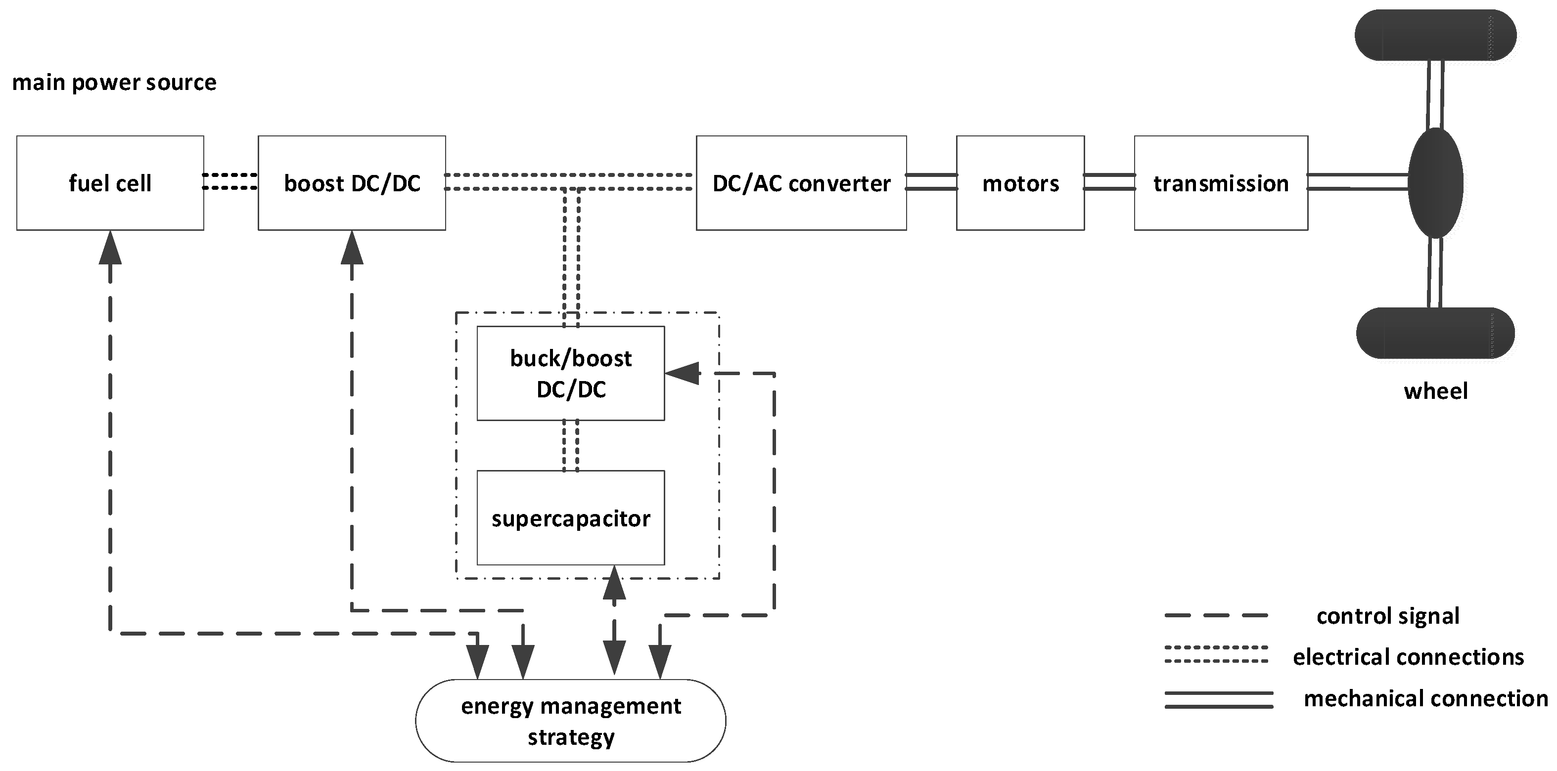
2.1. Fuel Cell Hybrid Powertrain Architecture

The block diagram of the structure of the FCHEV is shown in Figure 1. The FC is connected to a unidirectional DC/DC and the supercapacitor to a bidirectional DC/DC. The two are then connected in parallel to drive the motor that ultimately moves the wheel.

The main components of the FCHPS will be modeled in order to build a simulation system to carry out this study. Their modeling is discussed below.

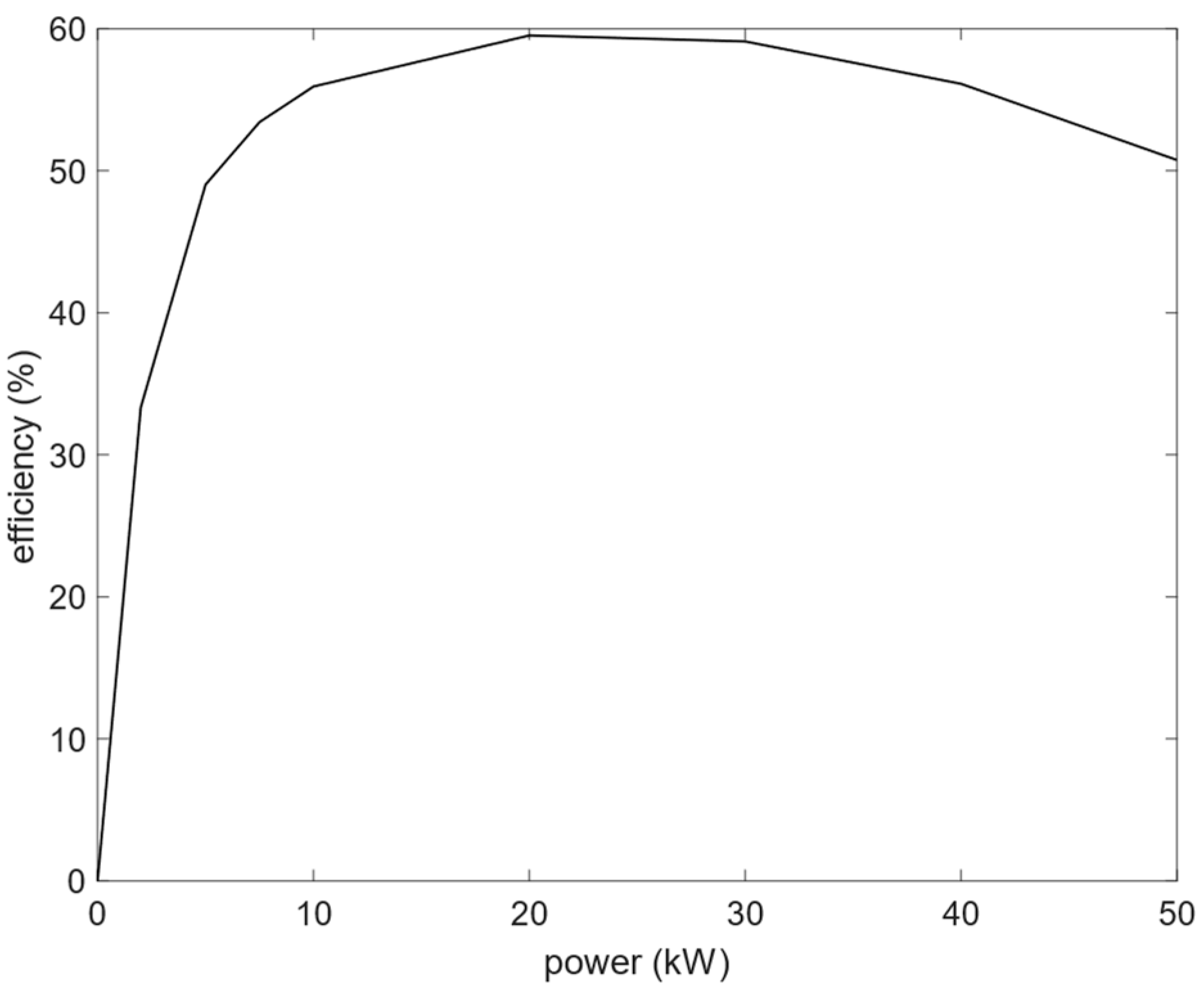
2.2. Fuel Cell Model

A Proton Exchange Membrane Fuel Cell (PEMFC) was chosen as the primary power source for the FCHEV. During the operation of the PEMFC, there are irreversible losses and a gradual drop in output voltage. These irreversible losses are reflected in the polarization overpotential, and the actual output voltage of the FC is determined by the polarization overpotential and the ideal electrical potential. The PEMFC monomer output voltage $V_{\mathit{cell}}$ is expressed as follows [29]:

$$V_{\mathit{cell}}=E_{Nernst}-V_{\mathit{act}}-V_{\mathit{ohm}}-V_{\mathit{con}}$$

(1)

where $E_{Nernst}$ is the ideal electric potential; $V_{\mathit{act}}$ is the activation overpotential; $V_{ohm}$ is the ohmic overpotential; and $V_{con}$ is the concentration difference overpotential.

The total voltage as well as the output power of the fuel cell stacks are

$$V_{fc}=N_{fc}{V}_{cell}$$

(2)

$$P_{fc,s}=I_{fc}{V}_{fc}$$

(3)

where $N_{fc}$ is the number of FC units connected in series; $V_{fc}$ and $I_{fc}$ are the total voltage and the current of the FC stacks, respectively; and $P_{fc,s }$ is the actual output power of the FC stacks.

To subsequently facilitate MLD modeling, the nonlinear PEMFC system needs to be linearized. The linearization takes into account the polarization curves, so that the input/output relationship for the FC is approximated as follows [30]:

$${\tau }_f{\dot{P}}_{fc,s}=k_f{P}_{fc,d}-P_{fc,s}$$

(4)

where ${\tau }_f$ is the time constant, here with a value of 0.2 s; $k_f$ is the gain factor, here with a value of 1; and $P_{fc,d}$ is the power required by the FC stacks.

The power efficiency curve of the FC is shown in Figure 2 [19]. It can be seen that the FC operates with relatively high efficiency when its output power is in the range of 7–50 kW, and therefore the powers in this range are identified as the high-efficiency zone of the FC.

2.3. Supercapacitor Model

The supercapacitor serves as an auxiliary energy source that can supply energy to the FCHEV or recover braking energy from the FCHEV. Based on its operating characteristics and using the classical equivalent circuit model, the output power of a single supercapacitor is as follows [31]:

$$\left\{\begin{array}{c}{P}_{\mathit{sc}}=U_{\mathrm{sc}}\times I_{\mathit{sc}}\\ U_{\mathit{sc}}=E_C-R_s\times I_{sc}\\ I_{\mathrm{sc}}=I_C+I_F\\ I_C=-C\frac{d{E}_C}{dt}\\ I_F=\frac{E_C}{R_F}\end{array}\right.$$

(5)

where $P_{\mathit{sc}}$ is the output power of the supercapacitor; $U_{\mathit{sc}}$ and $I_{\mathit{sc}}$ are the voltage and current of the supercapacitor, respectively; $E_c$ is the equivalent capacitance voltage; C is the capacity of the equivalent capacitor; $R_S$ is the charge/discharge resistance; $R_F$ is the self-discharge loss resistance; and $I_C$ and $I_F$ are the current values flowing through the equivalent capacitor and self-discharge loss resistance, respectively.

The supercapacitor state of charge (SOC) is calculated as follows [31]:

$$SOC=\frac{U_{sc}-U_{scmin}}{U_{scmax}-U_{scmin}}$$

(6)

where $U_{scmin}$ and $U_{scmax}$ are the minimum and maximum voltages of the supercapacitor, respectively.

2.4. DC/DC Model

The output power of the unidirectional DC/DC converter connected to the FC is

$$P_{d1}=P_{fc,s}{\eta }_{d1}$$

(7)

The output power of the bidirectional DC/DC converter connected to the supercapacitor is

$$P_{d2}=P_{\mathit{sc}}{\eta }_{d2}$$

(8)

where ${\eta }_{d1}$ and ${\eta }_{d2}$ are the efficiencies of the unidirectional and the bidirectional DC/DC converters, respectively.

2.5. Vehicle Dynamic Model

The required power of the motor in the driven state is

$$P_{m,d}=\frac{P_m}{{\eta }_m}$$

(9)

$$P_m=\frac{T_m{n}_m}{9550}$$

(10)

where $P_{m,d}$ is the gross motor power; $P_m$ and ${\eta }_m$ are the output mechanical power and the conversion efficiency of the motor, respectively; $T_m$ is the motor output torque; and $n_m$ is the actual motor output speed.

The motor power required for braking is similar to that for driving, and the power generated during braking can be calculated as follows:

$$P_{mec}=\frac{T_{mb}{n}_m}{9550}$$

(11)

$$P_{mb}=P_{mec}\cdot {\eta }_{mb}$$

(12)

where $P_{mec}$ is the braking mechanical power of the motor; $T_{mb}$ is the motor braking torque; ${\eta }_{mb}$ is the conversion efficiency of the motor as a generator; and $P_{mb}$ is the electrical energy generated during braking.

The dynamic response of the motor can be expressed linearly as

$${\tau }_m{\dot{T}}_m=k_m{T}_{m,d}-T_m$$

(13)

where ${\tau }_m$ is the motor time constant with a value of 1.1, and $T_{m,d}$ is the demanded torque of the motor.

The output torque of the motor is calculated based on the vehicle parameters and forces. According to the dynamic equations of vehicle driving, the forces on the vehicle during driving are

$$F_t=F_r+F_a+F_g+F_j$$

(14)

$$\left\{\begin{array}{c}{F}_r=fmg\mathit{cos}\theta \\ F_a=\frac{C_D{A}_f{v}_a^2}{21.15}\\ F_g=mg\mathit{sin}\theta \\ F_j=\beta m\frac{d{u}_a}{dt}\end{array}\right.$$

(15)

where $F_t$ is the driving force of the vehicle; $F_g$ is the grade resistance, $F_a$ is the air resistance, $F_j$ is the acceleration resistance, and $F_r$ is the rolling resistance to which the vehicle is subjected; $m$ is the mass of the whole vehicle; $\beta$ is the rotating mass conversion factor; $f$ is the wheel roll resistance coefficient; $A_f$ is the windward area; $v_a$ is the driving speed; $\theta$ is the road slope; and $C_D$ is the air resistance coefficient.

In

Table 1. Main technical parameters of FCHEV.

Name	Parameter/Unit	Numerical Value
Whole vehicle section	Total vehicle mass $\frac{m}{kg}$	1138
	Wind resistance coefficient $C_D$	0.335
	Windward area $\frac{A_f}{m^2}$	2
Tires	Wheel radius $\frac{r}{m}$	0.282
	Rolling resistance factor $f$	0.009
	Rotating mass conversion factor $\beta$	1
Motor drive	Maximum power $kW$	75
	Peak efficiency	0.92
Fuel cell	Maximum net power $kW$	50
	Peak efficiency	0.6
	Number of FC units $N_{fc}$	411
Supercapacitor	Capacity of equivalent capacitor C	2
	Charge/discharge resistance $R_S$	0.0026
	Self-discharge loss resistance $R_F$	965
	Rated voltage $V$	2
	Number of groups	80
DC/DC model	Efficiency of unidirectional DC/DC converter ${\eta }_{d1}$	96
	Efficiency of bidirectional DC/DC converter ${\eta }_{d2}$	97
Motor	Conversion efficiency of motor ${\eta }_m$	92
	Motor time constant ${\tau }_m$	1.1

, the main parameters of the FCHEV and the models are given out for the simulation application.

3. MLD Modeling of Fuel Cell Hybrid Powertrain

Regarding hybrid systems, Bemporad and Morari [32] proposed to utilize MLD models to describe such complex systems. The use of MLD models can centralize all the variables in the system and the relationships between the variables in a model framework that clearly reflects the dynamic logical relationships between the system variables, the switching of states, and the operational constraints. The relationships between the inputs, states, and outputs of the hybrid system can also be clearly established. The key to the modeling approach of the MLD model is logical propositions, which are mainly based on the logical rules of the system as well as qualitative knowledge. The logical propositions are then expressed as linear inequalities for integers and continuous variables.

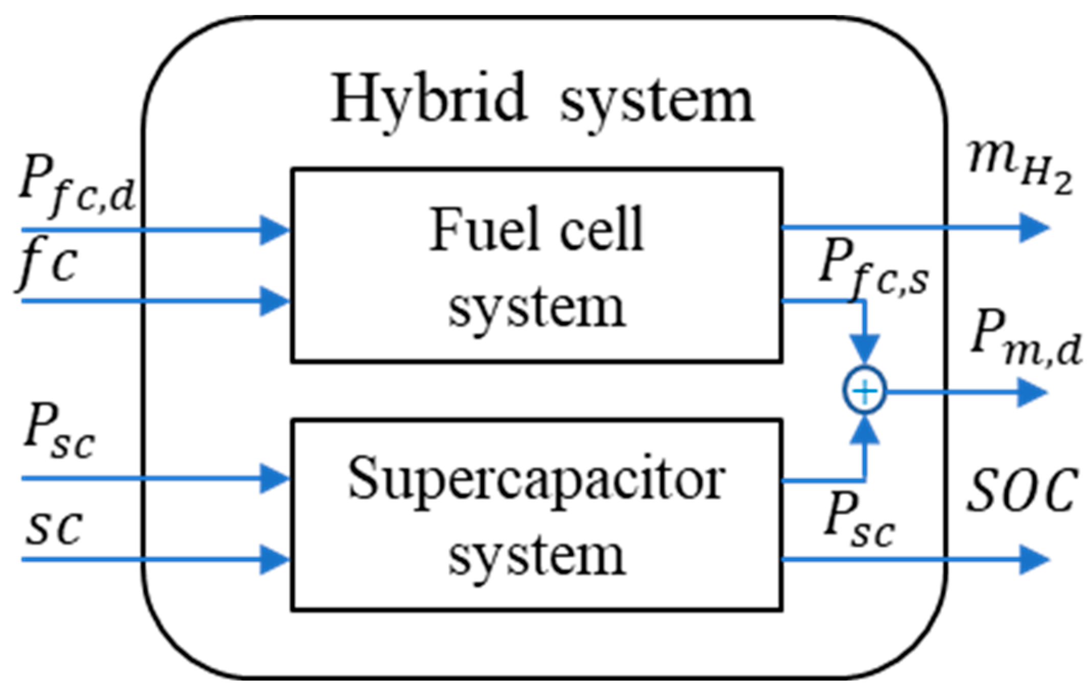
3.1. MLD Model Architecture of FCHPS

It is known from the above discussion that the FCHPS is mainly powered by the FC and supercapacitor, so there is a complex kinetic relationship among its various components. In order to effectively reduce fuel consumption, FC performance degradation, etc., it needs to be divided into different operating modes in the driving process of the FCHEV, and then the corresponding operating mode must be chosen according to the actual situation on the road. The operating modes of the FCHEV are shown in

Table 2. Operating modes defined for FCHEV.

Operating Mode	Fuel Cell Operating Conditions	Supercapacitor Operating Conditions
Joint driving	On	Discharge
Line charging	On	Charging
Separate driving for supercapacitor	Off	Discharge
Recovery of braking energy	Off	Charging

.

Simply using a combination of continuous and discrete-time dynamic variables makes it difficult to provide an accurate description of the system, and the MLD modeling approach can be used to bring together the complexity of multiple operating modes in this system in a single mathematical model. The analysis of the system shows that the generation of discrete variables in the FCHPS is mainly due to the on and off operation of the FC and supercapacitor, so the modeling framework shown in Figure 3 is used to represent the MLD model of the FCHPS, where $fc$ and $sc$ denote the Boolean quantities for the on and off states of the FC and supercapacitor, respectively, $u_b=[fc,sc{]}^{\mathrm{T}}$; and $m_{H_2}$ denotes the hydrogen consumption of the FC.

3.2. Hysdel-Based MLD Model Construction

In order to solve the inefficiency problem of traditional MLD modeling, Bemporad et al. [32] investigated the use of the Hysdel language for modeling. By using this method to model the hybrid system, the manual derivation process can be avoided, which saves time and improves the modeling efficiency to a great extent and ensures the accuracy of the model.

The Hysdel language consists of IMPLEMENTATION and INTERFACE, where INTERFACE is mainly used to detail variables such as inputs, outputs, and states of the system, while IMPLEMENTATION establishes relationships among variables. The modeling process has the following main steps:

1.

Definition of all variables in the system

According to the above analysis, the input variables of the MLD model are the demanded power of the FC and the output power of the supercapacitor, $\mathit{u}\left(k\right)=\left[P_{fc,d}\right(k),P_{sc}(k){]}^{\mathrm{T}}$; the output variables are the gross motor power, the hydrogen consumption, and the supercapacitor SOC, $\mathit{y}\left(k\right)=[P_{m,d}\left(k\right),m_{H_2}\left(k\right), SOC{]}^{\mathrm{T}}$; and the state variables are $\mathit{x}\left(k\right)=[P_{m,d}\left(k\right),m_{H_2}\left(k\right), SOC,t_{fc},t_{sc}{]}^{\mathrm{T}}$, where $t_{fc}$ and $t_{sc}$ are the discharge times of the FC and supercapacitor, respectively.

2.

Definition of system auxiliary variables

The main purpose of defining auxiliary variables is to be able to describe more accurately the constraints between the variables and the evolution process within the MLD model. Logical variables are defined according to linear affine constraints:

$${\mathit{\delta }}_e^k\left(k\right)=f\left(\mathit{x}\left(k\right),\mathit{u}\left(k\right),k\right)$$

(16)

According to the above equation, the logical variables are related to the state variable, the input variable, and the time, and they are the key to triggering the occurrence of the event. Based on the characteristics of the FC and supercapacitor, the trigger events of the FCHPS can be categorized into the following two types:

• The corresponding auxiliary discrete variables are set according to the threshold value of the FC (i.e., the FC high-efficiency region in Figure 2) and the magnitude of the discharge time, as follows:

When $P_{fc}\le 50 \mathrm{k}\mathrm{W}$, ${\delta }_e^1\left(k\right)=1$, otherwise ${\delta }_e^1\left(k\right)=0$;

When $P_{fc}\ge 7 \mathrm{k}\mathrm{W}$, ${\delta }_e^2\left(k\right)=1$, otherwise ${\delta }_e^2\left(k\right)=0$;

When $t_{fc}>5 \mathrm{s}$, ${\delta }_e^3\left(k\right)=1$, otherwise ${\delta }_e^3\left(k\right)=0$;

When $t_{fc}<25 \mathrm{s}$, ${\delta }_e^4\left(k\right)=1$, otherwise ${\delta }_e^4\left(k\right)=0$.

• The auxiliary discrete variables are set according to the charge state and the discharge time magnitude of the supercapacitor, as follows:

When $SOC>0.5$, ${\delta }_e^5\left(k\right)=1$, otherwise ${\delta }_e^5\left(k\right)=0$;

When $t_{sc}\ge 30 \mathrm{s}$, ${\delta }_e^6\left(k\right)=1$, otherwise ${\delta }_e^6\left(k\right)=0$;

When $t_{fc}\le 60 \mathrm{s}$, ${\delta }_e^7\left(k\right)=1$, otherwise ${\delta }_e^7\left(k\right)=0$.

The finite state machine model of the FCHEV dynamical system is a discrete state equation, mainly related to the binary of the individual components, the input control variables, and the above trigger events, which evolved from a logical state update function, which is a function of

$${\dot{\mathit{x}}}_b=h\left({\mathit{x}}_b,{\mathit{u}}_b,{\mathit{\delta }}_e\right)$$

(17)

where $h$ denotes the function associated with ${\mathit{x}}_b,{\mathit{u}}_b,{\mathrm{a}\mathrm{n}\mathrm{d} \mathit{\delta }}_e$.

Since there are four modes of operation, ${\mathit{x}}_{\mathit{b}}=\left[x_b^1,x_b^2,x_b^3,x_b^4\right]$, and the meaning of each quantity is shown below:

$x_b^1=fc\&sc$ means that both the FC and supercapacitor are on;

$x_b^2=fc\&{}^{\neg }sc$ means the FC is on and the supercapacitor is off;

$x_b^3={}^{\neg }fc\&sc$ means the FC is off and the supercapacitor is on;

$x_b^4={}^{\neg }fc\&{}^{\neg }sc$ means both the FC and supercapacitor are off.

Thus, the discrete dynamic mode $i\left(k\right)$ of the system is determined by ${\mathit{x}}_b$ and ${\mathit{\delta }}_e$.

3.

System operation constraints

To ensure that the optimal problem can obtain the optimal solution, it is necessary to impose the appropriate logical constraints on it:

$$\sum i\left(k\right)=1$$

(18)

In order to adapt to the characteristics of the supercapacitor and to work in a better state when the vehicle is in motion, the constraint is set for the supercapacitor SOC as follows [33]:

$$0.2\le SOC\le 0.8$$

(19)

Once the setup is completed following the steps described above, the MLD model of the FCHPS can be compiled by Hysdel to obtain its standard mathematical expression. The model obtained is a difference equation with five state variables, two input variables, two output variables, and the mixed-integer linear inequality constraint that should be satisfied among the variables, as follows:

$$\left\{\begin{array}{c}x\left(k+1\right)=Ax\left(k\right)+B_{3}z\left(k\right)\\ y\left(k\right)=Cx\left(k\right)+D_{3}z\left(k\right)\\ E_2\delta \left(k\right)+E_{3}z\left(k\right)\le E_{1}u\left(k\right)+E_{4}z\left(k\right)+E_5\end{array}\right.$$

(20)

where $z\left(k\right)$ refers to the auxiliary variables used in linking the discrete variables in the system to the continuous variables, $z\left(k\right)=\delta \left(k\right)u\left(k\right)$; and $\delta \left(k\right)$ is the logic variable, $\delta \left(k\right)\in \left\{\mathrm{0,1}\right\}$; the variable coefficient matrices $B_3:5\times 15, {\mathrm{D}}_3:3\times 15, E_1:68\times 2, E_2:68\times 3, E_3:68\times 15, E_4:68\times 15, \mathrm{a}\mathrm{n}\mathrm{d} E_5:68\times 1$ are not described in detail here because of their high dimensionality:

$$A=\left[\begin{array}{ccccc}-5& 0& 0& 0& 0\\ 0& -0.03125& 0& 0& 0\\ -0.00218& -2.4& 0.00218& 0& 0\\ 0& 0& 0& 0& 0\\ 0& 0& 0& 0& 0\end{array}\right], C=\left[\begin{array}{ccccc}1& 0& 0& 0& 0\\ 0& 1& 0& 0& 0\\ 0& 0& 1& 0& 0\end{array}\right].$$

4. Energy Management Strategy Based on MLD-MPC

When designing energy management strategies for the FCHPS, the fuel economy and hydrogen FC durability should be considered. To this end, it is necessary to obtain the equivalent hydrogen consumption of the FCHEV based on the operating characteristics of the key components and the consumption model. In order to improve the durability of the FC, it is necessary to quantify its lifetime degradation caused by variable load conditions, and thus to establish its degradation model. The details are discussed as follows.

4.1. Evaluation Indicators for Energy Management Strategies

4.1.1. Equivalent Hydrogen Consumption Model

By analyzing the working principle of the FC, it can be seen that in a dry external environment, its output current has a crucial influence on its hydrogen consumption, so the hydrogen consumption per unit of time can be calculated according to the following formula:

$$f_{H_2}=\frac{S_{H_2}{M}_{H_2}{N}_{fc}{I}_{fc}}{2000F}$$

(21)

where $S_{H_2}$ is the excess coefficient of hydrogen, $S_{H_2}=1.2$; $M_{H_2}$ is the molar mass of hydrogen, taken as $2 \mathrm{g}\cdot \mathrm{m}\mathrm{o}{\mathrm{l}}^{-1}$; and $N_{fc}$ is the number of FCs.

Thus, the real-time hydrogen consumption of the FC can be calculated as follows:

$$C_{H_2}\left(t\right)={\int }_0^t{f}_{H_2}dt$$

(22)

The equivalent 100 km hydrogen consumption $m_{H_2}$ is

$$m_{H_2}\left(t\right)=\frac{C_{H_2}}{s}\times 100$$

(23)

where $s$ indicates the traveling distance for the whole driving condition.

4.1.2. Degradation Model of FC

The performance degradation of the FC is mainly caused by changes in driving conditions such as idling, start/stop, variable load, and large load of the FCHFV, which are affected by the degree of each driving condition, as shown in Figure 4 [34]. From the figure, it can be observed that the lifetime of the FC is most affected by the two driving conditions of start/stop and variable load, so this paper mainly considers these two influence factors when establishing the degradation model.

By limiting the FC output power to operate within the high-efficiency zone, the effects of performance degradation due to start/stop conditions can be avoided. From the existing literature [35], for the effect of variable load conditions, the performance degradation rate $\rho$ of the FC can be solved by the standard deviation of the change in the FC output power over 5 s:

$$\rho \left(t\right)=-\frac{1}{3600}\left\{\left[225\sigma \left(P_{fc}^t,P_{fc}^{t-1},P_{fc}^{t-2},P_{fc}^{t-3},P_{fc}^{t-4}\right)+10\right]\right\}$$

(24)

where $P_{fc}^t$ is the output power of the FC at the current moment; $P_{fc}^{t-1},\cdots P_{fc}^{t-4}$ are the output powers of the FC in the adjacent 2~5 s, respectively; $t$ is the current moment of the FC working, $t=1,2,\cdots ,5$; and $\sigma$ is the standard deviation function.

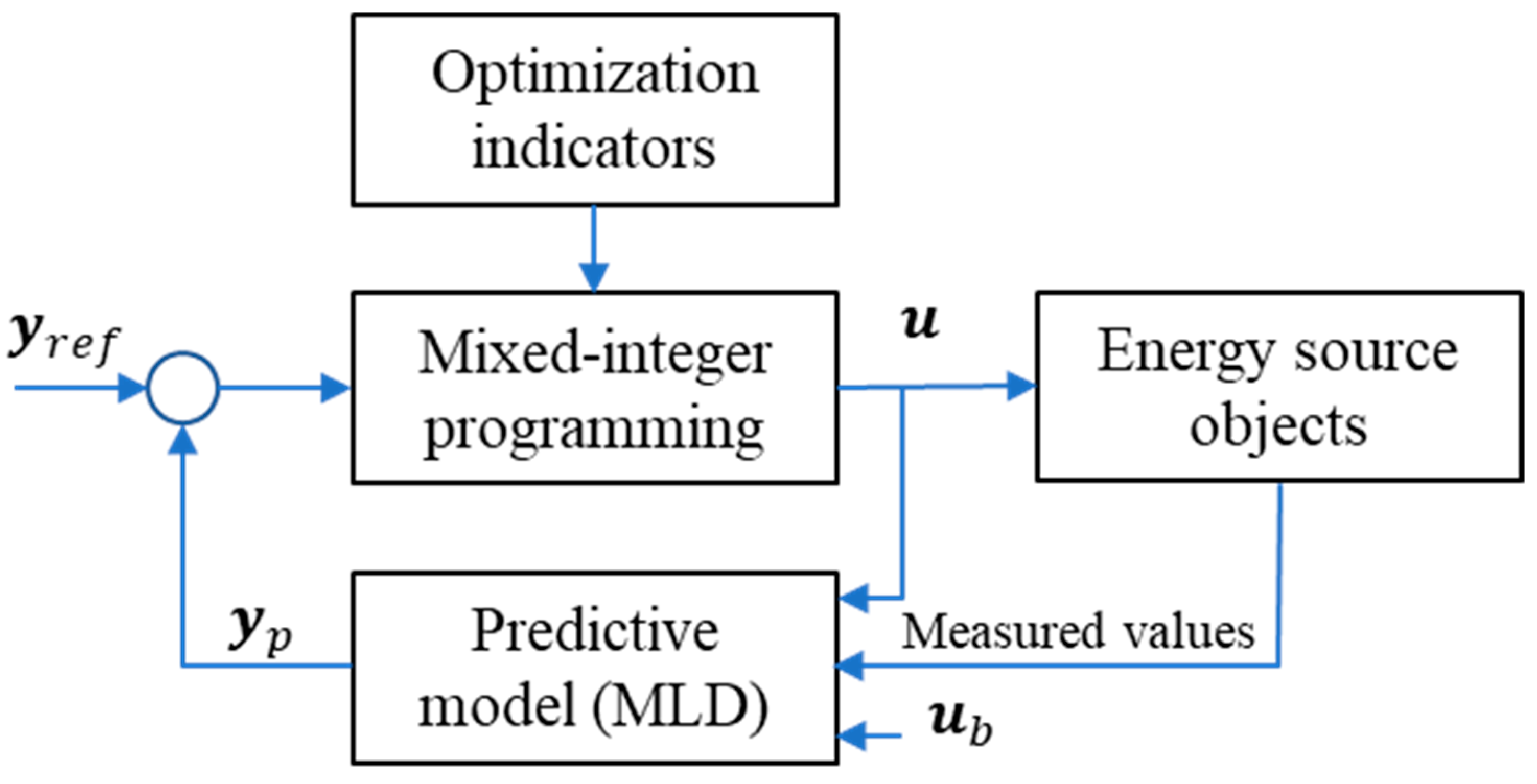
4.2. Energy Control Based on MLD-MPC

Figure 5 is the schematic diagram of MLD-MPC. It can be seen that the MLD-MPC-based energy management strategy includes the MLD model that is adopted as the predictive model, the optimization indicators, and the mixed-integer programming which is used to solve the corresponding optimization problem due to the introduction of MLD, where ${\mathit{y}}_{ref}\left(k\right)={\left[P_{req}\left(k\right), {SOC}_{ref}\left(k\right)\right]}^T$; $P_{req}$ is the whole vehicle required power calculated according to the driving conditions; $y_p\left(k\right)={\left[P_{m,d}\left(k\right),SOC\left(k\right)\right]}^T$ is the output of the predictive model; $\mathit{u}\left(k\right)=\left[P_{fc,d}\right(k),P_{sc}(k){]}^T$; and ${\mathit{u}}_b=[fc,sc{]}^T$.

When performing the optimization calculation, the supercapacitor SOC should be set in a reasonable range and the FC output power in the range of the high-efficiency zone, so that the optimization results obtained ensure that the whole vehicle has good dynamics. Based on the above considerations, the objective function is established as shown below:

$$L=Q{\left(m_{H_2}\left(t\right)\right)}^{2}dt+R{\left(\rho \left(t\right)\right)}^{2}dt$$

(25)

$$0.4\le SOC\le 0.8$$

(26)

$$7 \mathrm{kW}\le P_{fc}\le 50 \mathrm{kW}$$

(27)

According to the above equation, the objective function in the prediction time domain of the MPC used for optimization is

$$J=min{{\int }_t^{t+\Delta T}Q\left(m_{H_2}\left(t\right)\right)}^{2}dt+R{\left(\rho \left(t\right)\right)}^{2}dt$$

(28)

where $\mathsf{\Delta }T$ is the prediction interval; $Q$ and R denote the weight matrices.

The corresponding discrete objective function is established as shown in the following equation, where the reference values of hydrogen consumption and motor output power are both zero:

$$J\left(k\right)={\sum _{i=1}^{N_p}‖y_{ref}-y\left(k+i\right)‖}_Q^2+{\sum _{i=0}^{N_C-1}‖u\left(k+i\right)‖}_R^2$$

(29)

where $N_{p }$ is the prediction time domain; $N_c$ is the control time domain.

All the linear integer inequalities to be used by the FCHPS are already included in the established MLD model, associated with the objective function set above, and so the objective function of the FCHPS can be written as

$$\begin{gathered} \mathit{min}J\left[x\left(k\right),u\right]={\sum _{i=1}^{N_p}‖y_{ref}-y\left(k+i\right)‖}_Q^2+{\sum _{i=0}^{N_C-1}‖u\left(k+i\right)‖}_R^2 \\ subj.to.\left\{\begin{array}{c}x\left(k+1\right)=Ax\left(k\right)+B_{3}z\left(k\right)\\ y\left(k\right)=Cx\left(k\right)\\ \begin{array}{c}{E}_2\delta \left(k\right)+E_{2}z\left(k\right)\le E_{1}u\left(k\right)+E_{4}z\left(k\right)+E_5\\ \begin{array}{c}{x}_{min}\le x\left(k+j\right)\le x_{max}, j=0,1,\dots ,N_p\\ \begin{array}{c}{y}_{min}\le y\left(k+j\right)\le y_{max}, j=0,1,\dots ,N_p\\ u_{min}\le u\left(k+i\right)\le u_{max}, i=0,1,\dots ,N_c-1\end{array}\end{array}\end{array}\end{array}\right. \end{gathered}$$

(30)

Following the state space expression of Equation (20), the state prediction equation and output prediction equation in the prediction time domain can be further introduced as

$$\begin{array}{c}x\left(k+N_p\right)=A^{N_p}x\left(k\right)+{\displaystyle \sum _{i=0}^{N_p-1}}{A}^i\left[B_{1}u\right(k+N_p-1-i)+B_2\delta (k+N_p-1-i)\\ \hspace{1em}\hspace{1em}\hspace{1em}\hspace{1em}\hspace{1em}\hspace{1em} +\cdots +B_{3}z(k+N_p-1-i)]\\ y(k+N_p)=C{A}^{N_p}x(k)+{\displaystyle \sum _{i=0}^{N_p-1}}C{A}^i\left[B_{1}u\right(k+N_p-1-i)+B_2\delta (k+N_p-1-i)\\ \hspace{1em}\hspace{1em}\hspace{1em}\hspace{1em}\hspace{1em}\hspace{1em} +\cdots +B_{3}z(k+N_p-1-i)]+D_{1}u(k+N_p)+D_2\delta (k+N_p)\\ \hspace{1em}\hspace{1em}\hspace{1em}\hspace{1em}\hspace{1em}\hspace{1em} +D_{3}z(k+N_p)\end{array}$$

(31)

5. Simulation Test and Results Analysis

In order to verify the superiority of the proposed strategy in this paper, the control effects are compared with those of PFCS and CFCS [36] with real-time control. The following section mainly discusses the related simulation results and comparative analysis.

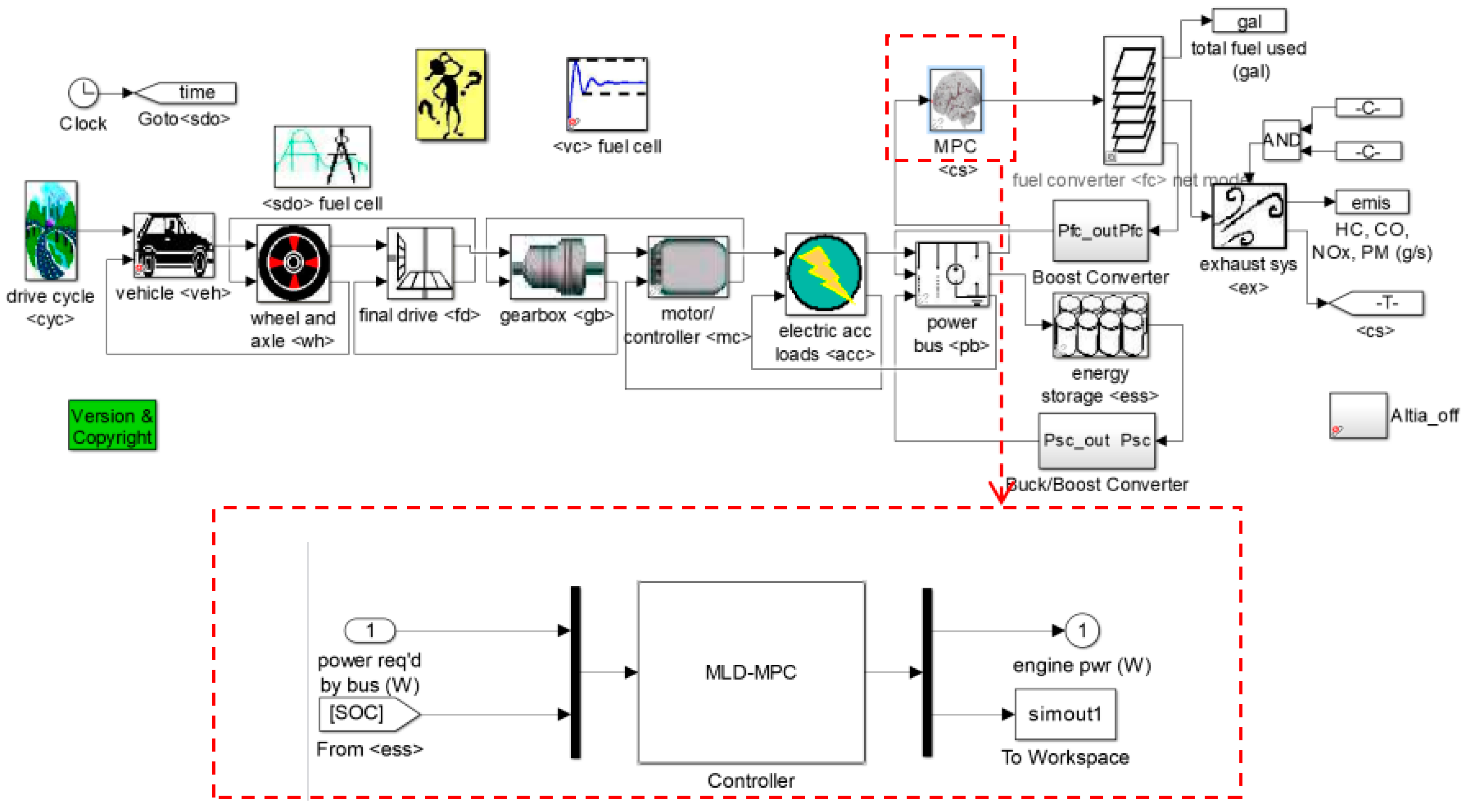
5.1. Simulation Model Construction

In this paper, Matlab/Simulink and Advisor 2002 software were used to jointly build the simulation model, shown in Figure 6. Advisor 2002 is the Advanced Vehicle Simulator which was mainly used to build the whole fuel cell vehicle power system, including the whole vehicle power model, fuel cell, supercapacitor, motor, power bus, management strategy, and other modules.

Table 3. The significance of each major module in Figure 6.

Name of the Module	Meaning
Drive cycle	Driving conditions of vehicle
Vehicle	Whole vehicle module
Wheel and axle	Wheel and axle of vehicle
Final drive	Main reducer
Gearbox	Mechanical gearbox
Motor/controller	Driving motor and its controller
Boost converter	Boost DC-DC converter
Buck/boost converter	Buck/boost DC-DC converter
Power bus	Direct current power bus
Electric acc loads	Electric accessory power calculation module
Energy storage	Supercapacitor
MPC <cs>	MLD-MPC control strategy
Fuel converter	Fuel cell
Exhaust system	Emission treatment module
<vc> fuel cell	Vehicle control module
<sdo> fuel cell	Data output module

gives the names of the modules and what they represent. As shown in the red dashed part in the figure, Simulink was used to build the MLD-MPC control strategy module. First, the control sequence of MLD-MPC was solved in Simulink using the MPT toolbox developed by the Bemporad A team, as well as by applying the state prediction equations, the input/output prediction equations, the optimization objective function, and the inequality constraints established above; second, its control sequence was ported to the Advisor control strategy module (MPC module) through function calls. The inputs to the control strategy module are the overall vehicle demand power and the SOC of the supercapacitor, and the output is the demand power of the fuel cell.

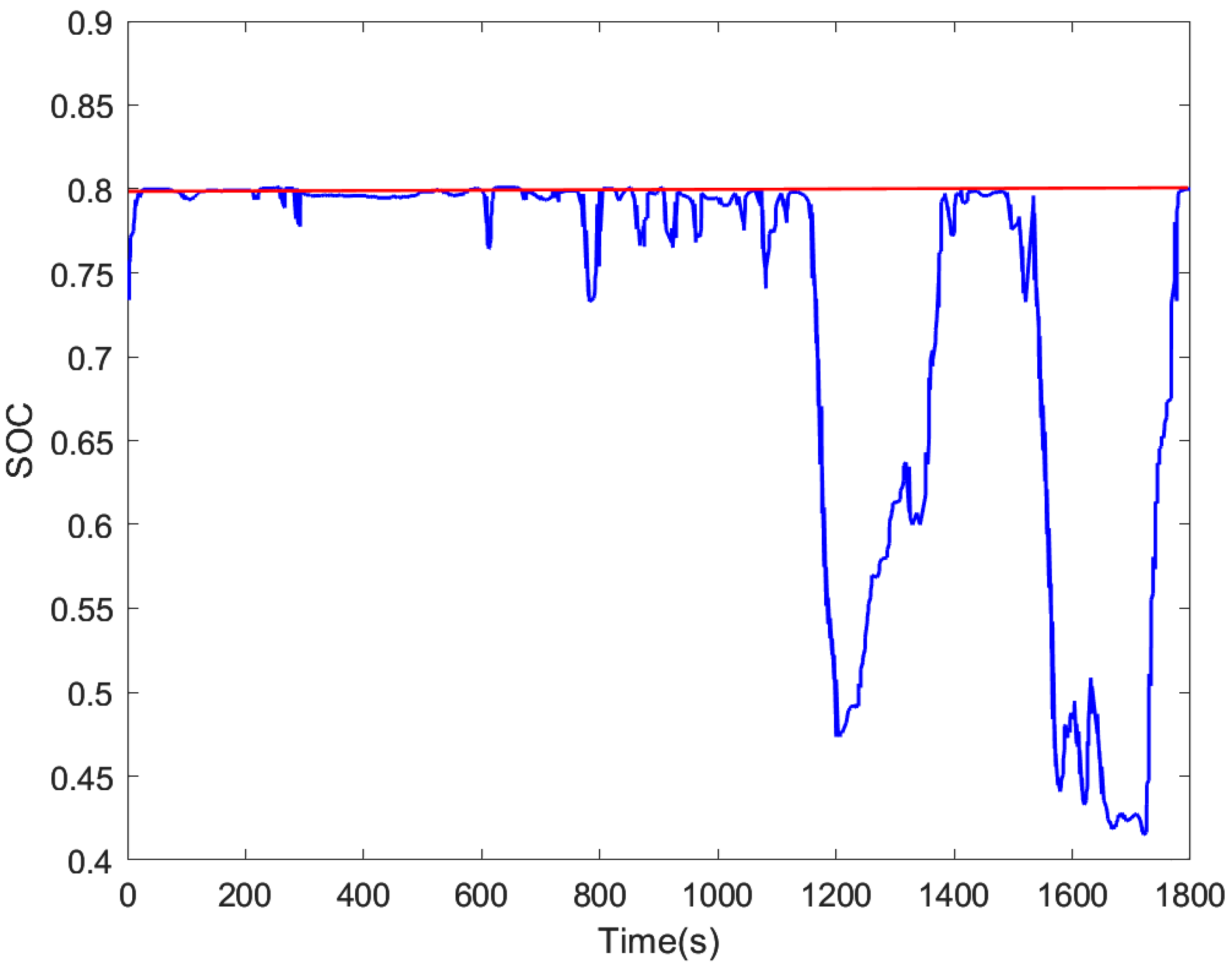
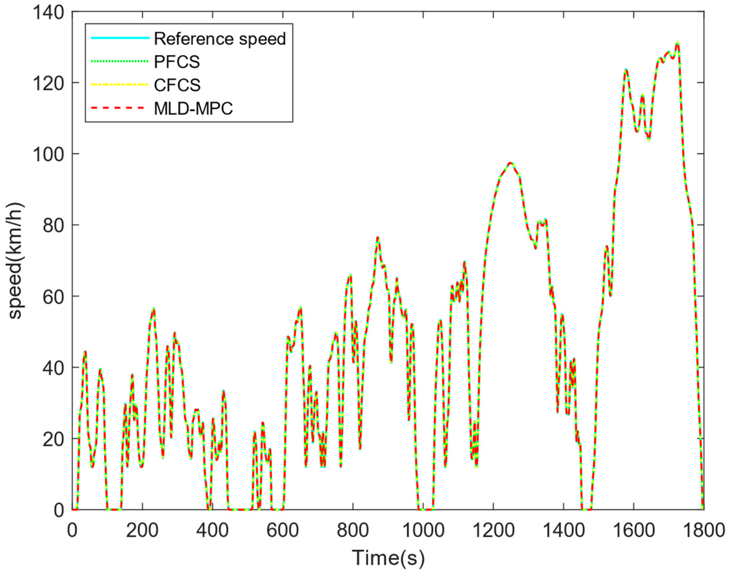
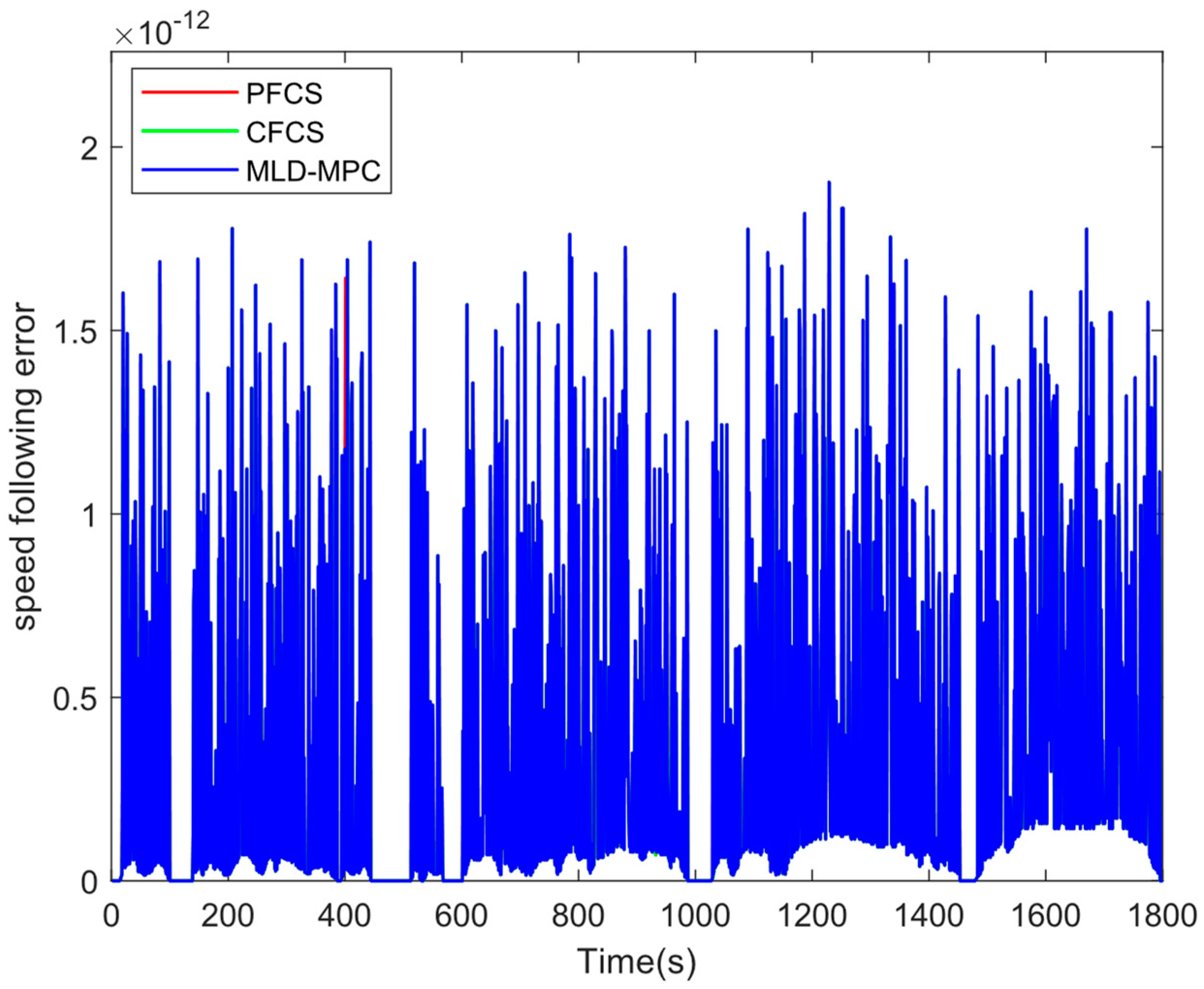
5.2. Dynamic Validation of Control Strategies

The World Light Vehicle Test Cycle (WLTC) is typically used for fuel consumption, electric consumption, and electric-only range testing, mainly covering urban, rural, ring road, and highway sections, and taking into account the driving congestion of vehicles. According to different driving speeds, the WLTC is divided into four parts—low speed, medium speed, high speed, and ultra-high speed—which is more in line with the actual driving of vehicles. Therefore, in order to better verify the accuracy of the model and the performance of the energy management strategy, the WLTC was selected for simulation and analysis. The specific information in the WLTC is shown in

Table 4. WLTC information.

Entry	Data
Driving time	1800 s
Distance traveled	23.27 km
Maximum speed	131.33 km/h
Average speed	46.51 km/h
Maximum acceleration	1.75 m/s2
Maximum deceleration	−1.5 m/s2
Average acceleration	0.42 m/s2
Average deceleration	−0.44 m/s2
Idle time	235 s
Number of starts and stops	8
Initial SOC for supercapacitors	70%

, including vehicle driving time, driving distance, maximum and average speed, maximum and average acceleration, maximum and average deceleration, and so on. The WLTC can simulate the road conditions of light vehicles.

The simulation experiments under the WLTC were carried out to validate the dynamics of the three control strategies, shown in Figure 7. From the figure, it can be seen that three real-time energy control strategies can accomplish the speed following curve requirements under the WLTC, and the following error is small, indicating that they can meet the dynamic requirements of the whole vehicle and verifying their effectiveness. As shown in Figure 8, speed following errors can be controlled within tolerance limits.

5.3. Analysis of Simulation Results

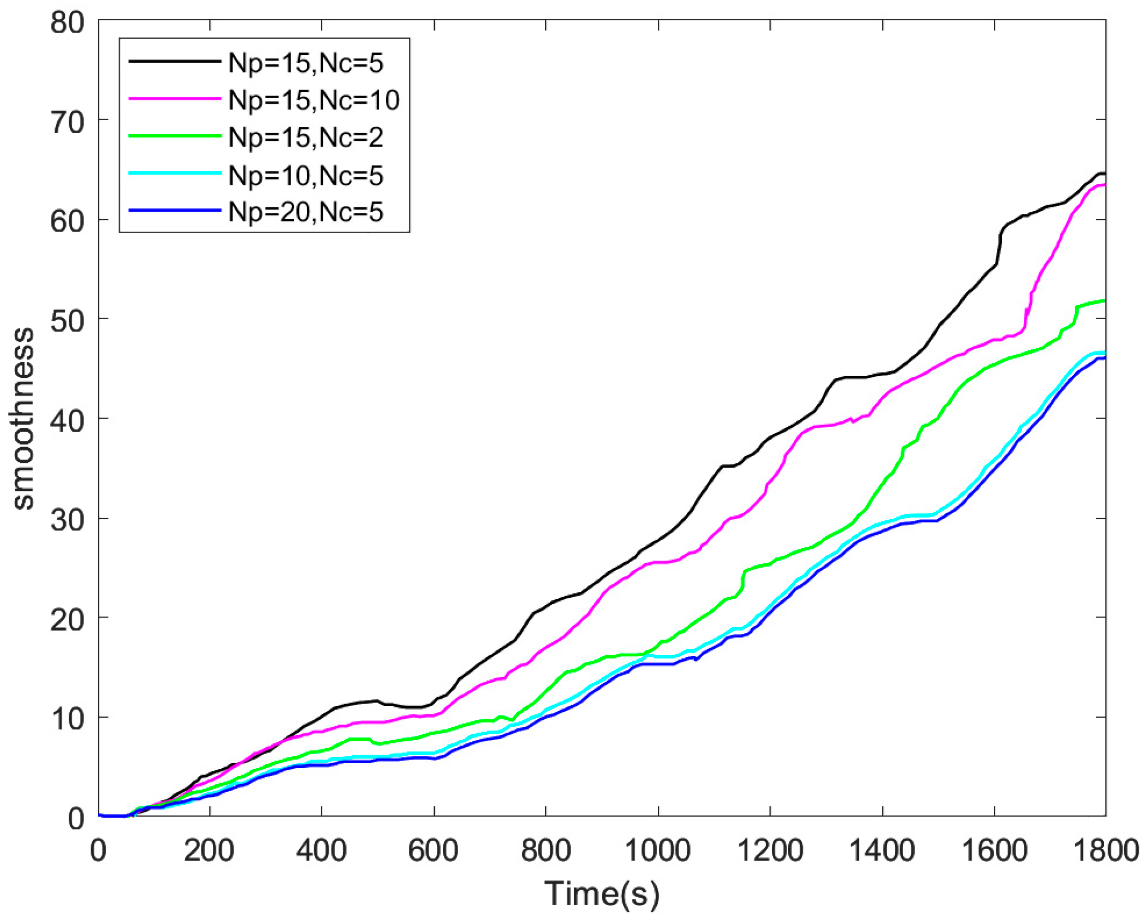
5.3.1. Parameter Selection for the Control Strategy

When the simulation experiments were carried out, the weight matrices of the objective function were chosen to be, respectively, as follows:

$$\begin{gathered} Q=[q{y}_{ij}{]}_{2\times 2}=\left\{\begin{array}{cc}q{y}_{ij}=25,& i=j=2\\ q{y}_{ij}=0,& \forall i,j \mathrm{a}\mathrm{n}\mathrm{d} i=j\ne 2\end{array}\right. \\ R=[r{x}_{ij}{]}_{5\times 5}=\left\{\begin{array}{cc}r{x}_{ij}=300,& i=j=2\\ q{x}_{ij}=0,& \forall i,j \mathrm{a}\mathrm{n}\mathrm{d} i=j\ne 2\end{array}\right. \end{gathered}$$

Different $N_p$ and $N_c$ values were selected for the simulation experiments, and the variation in hydrogen consumption obtained is shown in

Table 5. Hydrogen consumption for different values of $N_p$ and $N_c$.

Parameters	$\mathbf{Equivalent} \mathbf{Hydrogen} \mathbf{Consumption} \mathbf{per} \mathbf{Hundred} \mathbf{Kilometers}/\mathbf{L}\cdot 100 \mathbf{k}{\mathbf{m}}^{-1}$
$N_p=15,{ N}_c=2$	45.3
$N_p=15,{ N}_c=5$	44.6
$N_p=15,{ N}_c=10$	46.4
$N_p=10,{ N}_c=5$	45.7
$N_p=15,{ N}_c=5$	44.6
$N_p=20, N_c=5$	47.5

. From the table, it can be seen that when $N_p$ is the same and the value of $N_c$ is changed from small to large, the hydrogen consumption changes from large to small; however, when the value of $N_c$ is large to a certain extent, the hydrogen consumption will increase again. Therefore, the value of $N_c$ should be appropriate to obtain the best control effect. When $N_c$ is too large, the hydrogen consumption will increase, and the objective function solving process then requires a larger computational effort to increase the time. Similarly, when $N_c$ is the same, the change in the value of $N_p$ has the same effect on the hydrogen consumption control as in the above case.

The smoothness comparison curves of FC output power for different $N_p$ and $N_c$ values are shown in Figure 9. From the figure, it can be seen that although the output power is smoother for $N_p=15$, $N_c=10$, the hydrogen consumption is larger compared to $N_p=15$, $N_c=$ 5, and the system has a large amount of computation time and poor real-time performance. Based on the above analysis, considering the real-time performance, economy, and durability of the whole vehicle and the FC, $N_p=15$, $N_c=$5 is selected for simulation and analysis in this paper.

“Smoothness” is usually a relative concept that describes the degree of change, or the smoothness of the rate of change, of a physical quantity.

In order to quantify the degree of smoothness of the fuel cell output, the smoothness S of the fuel cell output power curve is defined as follows:

$$S=\frac{{\displaystyle {\int }_0^t\left|\frac{d{P}_{fc}}{dt}\right|dt}}{P_{MAX}}$$

where $P_{MAX}$ is the maximum net output power of the fuel cell.

As shown in Figure 9, the lower the smoothing value, the smoother the fuel cell output power, which will help to improve the durability of the fuel cell.

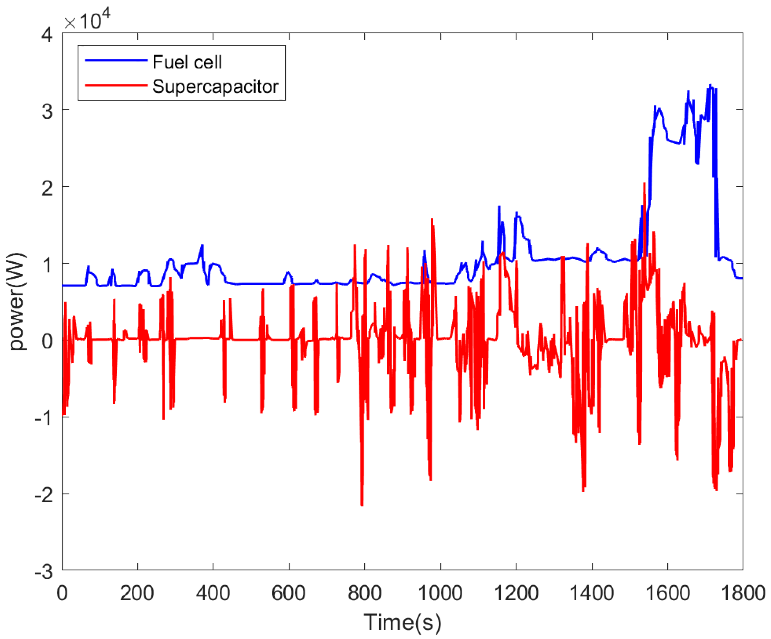
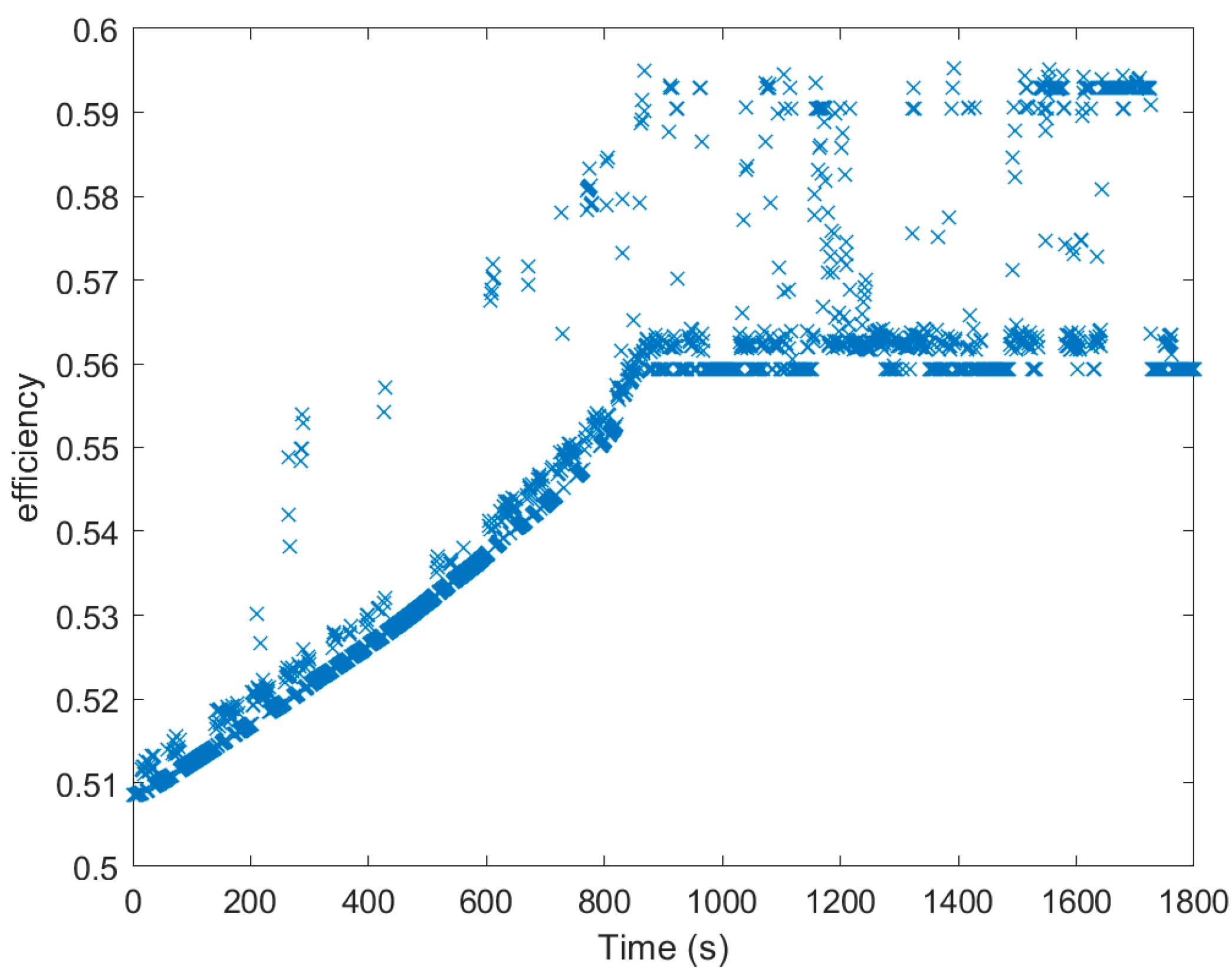
5.3.2. Results and Analysis

Under the MLD-MPC strategy, the variation curve of the supercapacitor SOC is shown in Figure 10; the variation curves of the output power of the FC and supercapacitor are shown in Figure 11. From the figures, it can be observed that the FC plays the role of the main power source and provides most of the energy in the whole driving process. When designing the MLD-MPC strategy, the output power of the FC is constrained in the high-efficiency area, so it can be seen from the figures that in the first 600 s when the demanded power of the whole vehicle is relatively small, the output power of the FC can meet the driving demands of the vehicle most of the time, and the output power of the supercapacitor is small and changes infrequently, and the change in its SOC is also relatively small; after 1200 s, as the driving conditions begin to enter the high-speed and ultra-high-speed stages, the demanded power of the whole vehicle will be correspondingly larger, so that the FC output power is larger, and the supercapacitor as an auxiliary energy source also provides part of the power, and its output power will be changed more frequently with the vehicle driving conditions. At the same time, the SOC fluctuates significantly during this time period. However, no matter how the driving conditions change, the change in SOC is always kept between 0.4 and 0.8 (note: the red line in Figure 10 indicates the upper limit of the SOC at 0.8, the blue indicates the SOC variation of supercapacitor), which is favorable for protecting the supercapacitor.

The real-time efficiency of the FC under the MLD-MPC strategy is shown in Figure 12. From the figure, it can be seen that the efficiencies of the proposed strategy are kept between 0.52 and 0.6 during the whole WLTC and the average efficiency is 0.57, all of which are in the high-efficiency area and can improve the economy of the whole vehicle. The variation curves of the FC output power under different control strategies are shown in Figure 13. As can be seen from the figure, during the whole WLTC, the number of FC starts/stops under the proposed strategy is zero, and the numbers under the PFCS and CFCS strategies are six and four, respectively. It has been shown [37] that the performance degradation of FCs is mainly related to the number of switches, fluctuation, and high-power runtime, so the proposed strategy is beneficial in prolonging the FC lifetime. Calculating the hydrogen consumption at 100 km ($\mathrm{L}\cdot 100 \mathrm{k}{\mathrm{m}}^{-1}$) under each control strategy, as shown in

Table 6. Comparison of simulation results of different energy management strategies.

Performance Indicators	PFCS	CFCS	MLD-MPC
$\mathrm{Equivalent} \mathrm{hydrogen} \mathrm{consumption} \mathrm{per} \mathrm{hundred} \mathrm{kilometers} \left(\mathrm{L}\cdot 100 \mathrm{k}{\mathrm{m}}^{-1}\right)$	50.1	45.5	44.6
Number of FC starts/stops	6	4	0
Average efficiency of FC	0.53	0.55	0.57
Average efficiency of supercapacitor	0.98	0.98	0.98

, it is 44.8 for MLD-MPC, and 50.1 and 45.4 for PFCS and CFCS, respectively, which are reduced by 10.98% and 1.98%, respectively; the average values of the real-time efficiency of the FC for PFCS and CFCS are 0.53 and 0.55. It is clear that the MLD-MPC strategy makes the FC have higher working efficiency.

6. Conclusions

In this paper, taking an FCHPS equipped with a hydrogen FC and supercapacitor as the research objective, an energy management strategy based on MLD-MPC is proposed, aiming to minimize hydrogen consumption and FC performance degradation under the premise of ensuring real-time optimization. The important findings are attached as follows:

• The Hysdel language is utilized to establish the MLD model of the FCHPS. Based on the mathematical modeling of the key components of the FCHPS, such as the FC, supercapacitor, DC/DC converters, and motor, the characteristics of different regions are described by the segment linearization method; the logic variables are used to organically link the different operating modes of the FCHPS with the constraints, logic rules, quantitative information, and charging/discharging operating modes of the segment linearization intervals, which are transformed into hybrid-integer linear inequalities. The inequalities are combined with the kinetic equations of each key component to establish the MLD model. The modeling problem for a complex hybrid system like the FCHPS is solved.
• The MLD-MPC energy management strategy for FCHEVs is established. Using the MLD model as a prediction model and the equivalent hydrogen consumption and the performance degradation of the FC as the optimization performance indexes, the economy of the FCHEV as well as the durability of the FC are improved and the real-time control of energy is achieved by rolling optimization of the operating states of the FC and the supercapacitor in the optimized finite time domain.
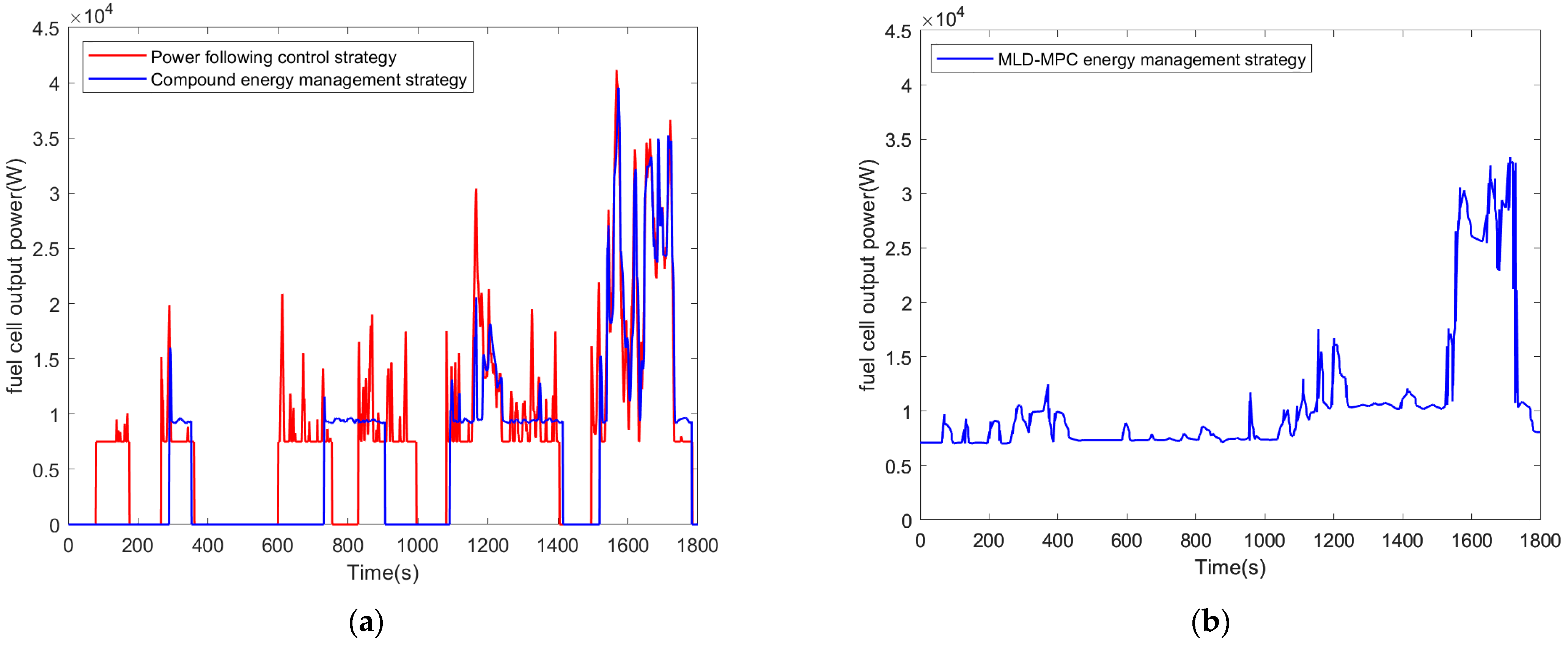
• Simulation verification under the WLTC shows that the hydrogen consumption of 100 km under the MLD-MPC energy management strategy proposed in this paper is 44.6 $\mathrm{L}\cdot 100 \mathrm{k}{\mathrm{m}}^{-1}$, which is 10.98% and 1.98% lower than the two types of real-time control strategies, PFCS and CFCS, respectively; and the number of start/stop times of the FC under the proposed strategy is reduced by six times and four times, respectively. So, the strategy in this paper has better economy and FC durability while achieving optimized real-time control.

In the future, we plan to carry out further research work, such as investigating energy management strategies for fuel cell hybrid vehicles equipped with three energy sources, and the application of explicit MPC instead of conventional MPC to provide better real-time performance.

References

1. World Energy Outlook 2021; International Energy Agency: Paris, France, 2021.
2. Djerioui, A.; Houari, A.; Zeghlache, S.; Saim, A.; Benkhoris, M.F.; Mesbahi, T.; Machmoum, M. Energy management strategy of supercapacitor/fuel cell energy storage devices for vehicle applications. Int. J. Hydrogen Energy 2019, 44, 23416–23428. [Google Scholar] [CrossRef]
3. Lü, X.; Wu, Y.; Lian, J.; Zhang, Y.; Chen, C.; Wang, P.; Meng, L. Energy management of hybrid electric vehicles: A review of energy optimization of fuel cell hybrid power system based on genetic algorithm. Energy Convers. Manag. 2020, 205, 112474. [Google Scholar] [CrossRef]
4. Chen, W.R.; Li, J.C.; Li, Q. Power following control strategy for SOC dynamic regulation of fuel cell small vehicles. J. Southwest Jiaotong Univ. 2021, 56, 197–205. [Google Scholar]
5. Li, D.; Xu, B.; Tian, J.; Ma, Z. Energy management strategy for fuel cell and battery hybrid vehicle based on fuzzy logic. Processes 2020, 8, 882. [Google Scholar] [CrossRef]
6. Zhou, W.; Yang, L.; Cai, Y.; Ying, T. Dynamic programming for new energy vehicles based on their work modes Part II: Fuel cell electric vehicles. J. Power Sources 2018, 407, 92–104. [Google Scholar] [CrossRef]
7. Sorlei, I.S.; Bizon, N.; Thounthong, P.; Varlam, M.; Carcadea, E.; Culcer, M.; Iliescu, M.; Raceanu, M. Fuel Cell Electric Vehicles—A Brief Review of Current Topologies and Energy Management Strategies. Energies 2021, 14, 252. [Google Scholar] [CrossRef]
8. Li, X.; Wang, Y.; Yang, D.; Chen, Z. Adaptive Energy Management Strategy for Fuel Cell/Battery Hybrid Vehicles using Pontryagin’s Minimal Principle. J. Power Sources 2019, 440, 227105. [Google Scholar] [CrossRef]
9. Meng, X.; Li, Q.; Chen, W.R.; Zhang, G.R. A hierarchical energy management method for fuel cell hybrid power systems based on the Pontryagin Minimum Principle for satisfactory optimization. Chin. J. Electr. Eng. 2019, 39, 782–792+957. [Google Scholar]
10. Tribioli, L.; Cozzolino, R.; Chiappini, D.; Iora, P. Energy management of a plug-in fuel cell/battery hybrid vehicle with on-board fuel processing. Appl. Energy 2016, 184, 140–154. [Google Scholar] [CrossRef]
11. Wang, Z.; Xie, Y.; Zang, P.; Wang, Y. Energy management strategy for fuel cell buses based on the principle of minimal value. J. Jilin Univ. (Eng. Ed.) 2020, 50, 36–43. [Google Scholar]
12. Zhang, F.; Hu, X.; Xu, K. Status and prospects of research on model predictive energy management for hybrid vehicles. J. Mech. Eng. 2019, 55, 86–108. [Google Scholar] [CrossRef]
13. Vahidi, A.; Stefanopoulou, A.; Peng, H. Current management in a hybrid fuel cell power system: A model-predictive control approach. IEEE Trans. Control Syst. Technol. 2006, 14, 1047–1057. [Google Scholar] [CrossRef]
14. Carignano, M.G.; Costa-Castelló, R.; Roda, V.; Nigro, N.M.; Junco, S.; Feroldi, D. Energy management strategy for fuel cell-supercapacitor hybrid vehicles based on prediction of energy demand. J. Power Sources 2017, 360, 419–433. [Google Scholar] [CrossRef]
15. Zhao, Z.; Shen, P.; Jia, Y.; Zhou, L. Model predictive real-time optimal control for fuel cell car. J. Tongji Univ. (Nat. Sci.) 2018, 46, 648–657. [Google Scholar]
16. Bambang, R.T.; Rohman, A.S.; Dronkers, C.J.; Ortega, R.; Sasongko, A. Energy management of fuel cell/battery/supercapacitor hybrid power sources using model predictive control. IEEE Trans. Ind. Inform. 2014, 10, 1992–2002. [Google Scholar]
17. Li, T.; Liu, H.; Wang, H.; Yao, Y. Hierarchical predictive control-based economic energy management for fuel cell hybrid construction vehicles. Energy 2020, 198, 117327. [Google Scholar] [CrossRef]
18. Zhou, Y.; Li, H.; Ravey, A.; Péra, M.C. An integrated predictive energy management for light-duty range-extended plug-in fuel cell electric vehicle. J. Power Sources 2020, 451, 227780. [Google Scholar] [CrossRef]
19. Zhou, Y.; Ravey, A.; Péra, M.C. Real-time cost-minimization power-allocating strategy via model predictive control for fuel cell hybrid electric vehicles. Energy Convers. Manag. 2021, 229, 113721. [Google Scholar] [CrossRef]
20. Shen, D.; Lim, C.C.; Shi, P. Robust fuzzy model predictive control for energy management systems in fuel cell vehicles. Control Eng. Pract. 2020, 98, 104364. [Google Scholar] [CrossRef]
21. Pereira, D.F.; Lopes, F.; Watanabe, E.H. Nonlinear model predictive control for the energy management of fuel cell hybrid electric vehicles in real-time. IEEE Trans. Ind. Electron. 2020, 68, 3213–3223. [Google Scholar] [CrossRef]
22. Yue, M.; Jemei, S.; Gouriveau, R.; Zerhouni, N. Review on health-conscious energy management strategies for fuel cell hybrid electric vehicles: Degradation models and strategies. Int. J. Hydrogen Energy 2019, 44, 6844–6861. [Google Scholar] [CrossRef]
23. Zhang, Y. Research on Modeling and Control Methods for Hybrid Systems. Master’s thesis, North China Electric Power University, Baoding, China, 2008.
24. Li, J.F.; Tang, T.H.; Yao, G. Modeling and energy-saving control of common DC bus AC drive systems based on hybrid Petri networks. Power Syst. Prot. Control 2011, 39, 1–6. [Google Scholar]
25. Li, X.; Xu, J.Q. Modeling and control of bidirectional ICPT systems based on hybrid automata. Power Autom. Equip. 2022, 42, 107–113. [Google Scholar]
26. Sun, X.; Wu, P.; Cai, Y.; Wang, S.; Chen, L. Piecewise affine modeling and hybrid optimal control of intelligent vehicle longitudinal dynamics for velocity regulation. Mech. Syst. Signal Process. 2022, 162, 108089. [Google Scholar] [CrossRef]
27. Chen, J.; Lin, C.; Liang, S. Mixed logical dynamical model-based MPC for yaw stability control of distributed drive electric vehicles. Energy Procedia 2019, 158, 2518–2523. [Google Scholar] [CrossRef]
28. Lian, J.; Liu, S.; Li, L.; Liu, X.; Zhou, Y.; Yang, F.; Yuan, L. A Mixed Logical Dynamical-Model Predictive Control (MLD-MPC) Energy Management Control Strategy for Plug-in Hybrid Electric Vehicles (PHEVs). Energies 2017, 10, 74. [Google Scholar] [CrossRef]
29. Jiang, K.; Guo, S.H.; Wu, Q.H. Matching and optimization of power system parameters for fuel cell sightseeing vehicles. Sci. Technol. Eng. 2019, 19, 351–356. [Google Scholar]
30. Arce, A.; del Real, A.J.; Bordons, C. MPC for battery/fuel cell hybrid vehicles including fuel cell dynamics and battery performance improvement. J. Process Control. 2009, 19, 1289–1304. [Google Scholar] [CrossRef]
31. Zhang, R.; Tao, J.; Zhou, H. Fuzzy Optimal Energy Management for Fuel Cell and Supercapacitor Systems Using Neural Network Based Driving Pattern Recognition. IEEE Trans. Fuzzy Syst. 2018, 27, 45–57. [Google Scholar] [CrossRef]
32. Bemporad, A.; Morari, M. Control of systems integrating logic, dynamics, and constraints. Automatica 1999, 35, 407–427. [Google Scholar] [CrossRef]
33. Chan, C.C.; Bouscayrol, A.; Chen, K. Electric, hybrid, and fuel-cell vehicles: Architectures and modeling. IEEE Trans. Veh. Technol. 2010, 59, 589–598. [Google Scholar] [CrossRef]
34. Pei, P.; Chen, H. Main factors affecting the lifetime of proton exchange membrane fuel cells in vehicle applications: A review. Appl. Energy 2014, 125, 60–75. [Google Scholar] [CrossRef]
35. Fowler, M.W.; Mann, R.F.; Amphlett, J.C.; Peppley, B.A.; Roberge, P.R. Incorporation of voltage degradation into a generalised steady state electrochemical model for a PEM fuel cell. J. Power Sources 2002, 106, 274–283. [Google Scholar] [CrossRef]
36. Lin, C.; Luo, W.; Lan, H.; Hu, C. Research on Multi-Objective Compound Energy Management Strategy Based on Fuzzy Control forFCHEV. Energies 2022, 15, 1721. [Google Scholar] [CrossRef]
37. Pei, P.C.; Chang, Q.F.; Tang, T. A quick evaluating method for automotive fuel cell lifetime. Int. J. Hydrogen Energy 2008, 33, 3829–3836. [Google Scholar] [CrossRef]
Figure 1. System structure of FCHEV.
Wevj 15 00151 g001
Figure 2. Power efficiency curve of FC.
Wevj 15 00151 g002
Figure 3. MLD model framework.
Wevj 15 00151 g003
Figure 4. The performance degradation degree of the FC by various drive cycles.
Wevj 15 00151 g004
Figure 5. The schematic diagram of MLD-MPC.
Wevj 15 00151 g005
Figure 6. The simulation model of the EMS based on the MLD-MPC control strategy.
Wevj 15 00151 g006
Figure 7. Speed following curves under WLTC.
Wevj 15 00151 g007
Figure 8. Speed following errors under WLTC.
Wevj 15 00151 g008
Figure 9. The smoothness comparison curves of the FC output power for different values of Np and Nc.
Wevj 15 00151 g009
Figure 10. SOC variation curve of supercapacitor.
Wevj 15 00151 g010
Figure 11. The output power curves of the FC and supercapacitor.
Wevj 15 00151 g011
Figure 12. Real-time efficiency of FC under MLD-MPC.
Wevj 15 00151 g012
Figure 13. The variation curves of FC output power under different control strategies: (a) PFCS and CFCS; (b) MLD-MPC.
Wevj 15 00151 g013