Abstract
In order to reduce energy consumption, improve driving mileage, and make vehicles adopt driver styles, research on automatic optimization of control strategy based on driver style is conducted in this paper. According to the structure of the powertrain, the vehicle control strategy is designed and a driver-style recognition model based on fuzzy recognition is added to the rule-based control strategy to improve the driver adaptation of the vehicle. In order to further improve the energy-saving effect of the strategy, the control strategy based on driver style is automatically optimized by the Isight optimization platform to make the strategy reach optimum. The test results show that the strategy based on driver style is able to adapt to different styles of drivers and the economy of the vehicle is improved by 2.06% compared with pre-optimization, which validates the effectiveness of the strategy.
1. Introduction
The dynamics and economy have always been the evaluation index of the performance of electric vehicles, good dynamics can meet the demand for rapid acceleration in the driving process, and good economy can meet the demand of the long mileages of vehicles [1,2]. However, due to the difference in the efficiency of the motor at various working points, resulting in the unavoidable contradiction between the dynamics and economy of vehicles, a reasonable vehicle control strategy for electric vehicles can, to a certain extent, balance the demand of the two at different moments and adjust the contradiction between the two [3,4,5]. Therefore, most researchers have focused on the improvement in the vehicle control strategy. Ref. [6] carried out the division of working modes as well as the allocation of speed and torque of coupled modes based on the principle of minimum electric power by calculating the demand torque in the dynamic mode and economic mode. Ref. [7] optimized and analyzed the control strategy of the dual-motor powertrain with the objectives of minimum energy consumption and mode switching frequency and obtained the working points and allocation strategies of power about the motor in different working modes. Ref. [8] analyzed and calculated the demand torque and compensation torque on the basis of the proposed framework of control strategy and analyzed the allocation of torque of the two motors in the coupled mode. Ref. [9] proposed a new two-motor coupling configuration and analyzed its four strategies of mode switching and the simulation results show that the two-motor powertrain has higher energy utilization than a single-motor powertrain. Ref. [10] took the friction limit of the front and rear wheels as an optimization objective in order to obtain the driving/braking distribution coefficient of the front and rear axles, improving the driving stability of the vehicle. Ref. [11] designed a dual fuzzy controller to optimize the torque allocation in the EV mode and used a Genetic Algorithm to improve the comprehensive efficiency of the system by multi-objective optimization for the control rules of the system. Ref. [12] determined the relationship between the torque and the efficiency of the motor at a given speed by building a loss model of the motor and formulated the corresponding torque allocation strategy and optimization scheme. Ref. [13] proposed a braking distribution strategy taking parallel hybrid vehicles as the research object and analyzed the influencing factor of the regenerative braking system through simulation. Ref. [14] proposed a control strategy to allocate the electric and mechanical braking force according to the braking strength and the electric motor first provides as much electric braking force as possible during braking; the insufficient part is supplemented by the mechanical braking force.
But most control strategies are not adapted to different types of drivers [15]. Because different drivers have different driving styles when driving and have different power demands under a certain driving cycle, the power adaptability of the vehicle is poor. For this reason, scholars have conducted a series of research on driver style recognition. Ref. [16] mainly explored the methods of driver style recognition and trained the model of driver style recognition by a fuzzy neural network to get fuzzy inference rules and recognize the driver style. Ref. [17] took the average value of acceleration and the standard deviation of acceleration as the inputs of fuzzy identification of driver style and the output is the influence coefficient of power demand. Accelerator pedal opening, velocity, and the influence coefficient of power demand are used to determine the discharge power of the battery together. The influence coefficient of power demand is different for drivers with different styles, so as to achieve the self-adaptation of driver styles.
Therefore, in this paper, in order to improve the overall performance of the vehicle, taking the dual-motor powertrain of an 18-ton city bus as the research object, a driving control strategy based on the principle of prioritizing high-efficiency motor as well as a braking control strategy of the distribution of multilevel braking force are first designed. Then, in order to enhance the adaptability of the vehicle to different types of drivers, fuzzy identification of driver style is conducted by the average value of acceleration and standard deviation of acceleration; fuzzy identification of acceleration intention is conducted by accelerator pedal opening and its changing rate, then the recognition results of driver style and acceleration intention are used as inputs to the fuzzy controller of torque correction coefficient k to correct the driving demand torque by k value outputted through defuzzification to get a more accurate demand torque that adapts driver style, which makes the powertrain work in a more reasonable working mode. Finally, the strategy based on driver style is automatically optimized by the Isight optimization platform to make the strategy reach optimum. Test results show that the strategy based on driver style can adapt to different types of drivers and the economy of the optimized strategy is further improved.
2. Dual-Motor Powertrain Configuration
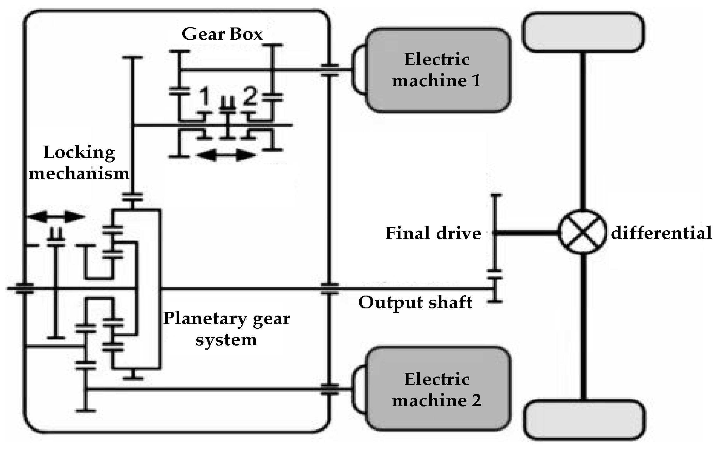
The dual-motor powertrain of the 18 tons city bus is taken as the research object and the configuration of the powertrain is shown in Figure 1, which consists of a planetary gear system, two-gear gearbox, electric machine 1, electric machine 2, and so on. Table 1 shows the basic parameters of the dual-motor powertrain and the vehicle.

Figure 1.
Configuration of the dual-motor powertrain.

Table 1.
The basic parameters of the powertrain and the vehicle.
For the dual-motor powertrain, the two input shafts of the system are the output shafts of the two motors and the output shafts of the system are connected to the ring gear of the planetary row. The planetary rack is fixed to the powertrain body by a locking mechanism and motor 2 is connected to the sun wheel via an idler pulley; the torque is loaded on the ring gear through the planetary pulley, which in turn transfers the power to the output shaft to ultimately drive the rear axle. The reduction ratio of motor 2 to the output shaft of the system is fixed, i.e., the transmission ratio of the planetary row in this structure. While the torque of motor 1 is loaded on the ring gear through the two-gear transmission, the reduction ratio of motor 1 to the output shaft of the system varies according to the gear.
3. Research on Vehicle Control Strategy
3.1. Research on Driving Control Strategy
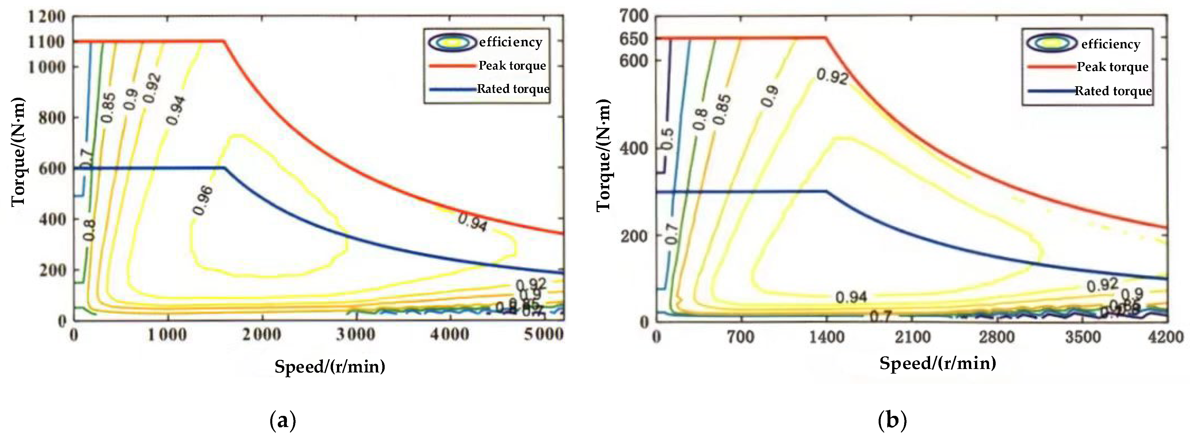
In this paper, the working modes of dual-motor powertrain are divided into three types according to the driving cycle of the vehicle: motor 1 alone, motor 2 alone, and dual-motor co-driving. The control strategy mainly consists of three parts: demand torque calculation, working modes recognition, and demand torque distribution [18]. As shown in Figure 2a, the high-efficiency zone of motor 1 is concentrated in the middle and high-speed region of 1300~3100 r/min, the corresponding velocity is 10~27 km/h when the transmission is on the first gear, and 28~68 km/h when the transmission is on the second gear. As shown in Figure 2b, the high-efficiency zone of motor 2 is concentrated in the middle and low-speed region of 900~2500 r/min and the corresponding velocity is 17~49 km/h [19].
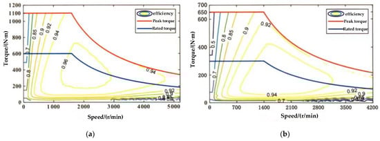
Figure 2.
(a) The efficiency map of the motor 1; (b) The efficiency map of the motor 2.
Therefore, when the transmission is in the first gear, when the velocity is less than 17 km/h, the efficiency of motor 1 is higher; when the velocity is more than 27 km/h, the efficiency of motor 2 is higher; and when the velocity is between 17 and 27 km/h, the efficiency of motor 1 and motor 2 is both relatively high, taking into account that the demand torque of the vehicle in the low-speed zone of 17~27 km/h on the low-gear position is larger, the efficiency of the corresponding motor 1 is higher at this time [20]. Therefore, motor 1 can be considered as a preferred choice. When the transmission is in the second gear, when the velocity is less than 28 km/h, motor 2 is more efficient; when the velocity is more than 49 km/h, motor 1 is more efficient; and when the velocity is between 28 and 49 km/h, both motor 1 and motor 2 are relatively efficient, considering that the demand torque of the vehicle in the middle and high-speed zone of 28~49 km/h on the high-gear position is smaller, at this time, the efficiency of the corresponding motor 2 is higher. Therefore, motor 2 can be considered as a preferred choice [21].
In order to improve the overall efficiency of the dual-motor powertrain, according to the current gear, velocity, and actual driving demand torque, based on the principle of prioritizing the high-efficiency motor to select the working mode and allocate the outputting torque, so as to ensure that motor 1 and 2 work in the high-efficiency zone as much as possible. The specific strategy is designed as shown in Table 2.
Table 2.
Strategy of torque distribution for dual-motor powertrain.
In the table, V denotes the speed of the vehicle, is the demand torque of the vehicle depending on the opening of the accelerator pedal, is the maximum torque at the current speed of motor 1, is the maximum torque at the current speed of motor 2, is the actual torque provided by motor 1, is the actual torque provided by motor 2, is the rated torque of motor 1, is the rated torque of motor 2, and and are the gear ratio of the transmission on the first and second gear, respectively. is a characteristic parameter of the planetary row.
3.2. Research on the Regenerative Braking Control Strategy
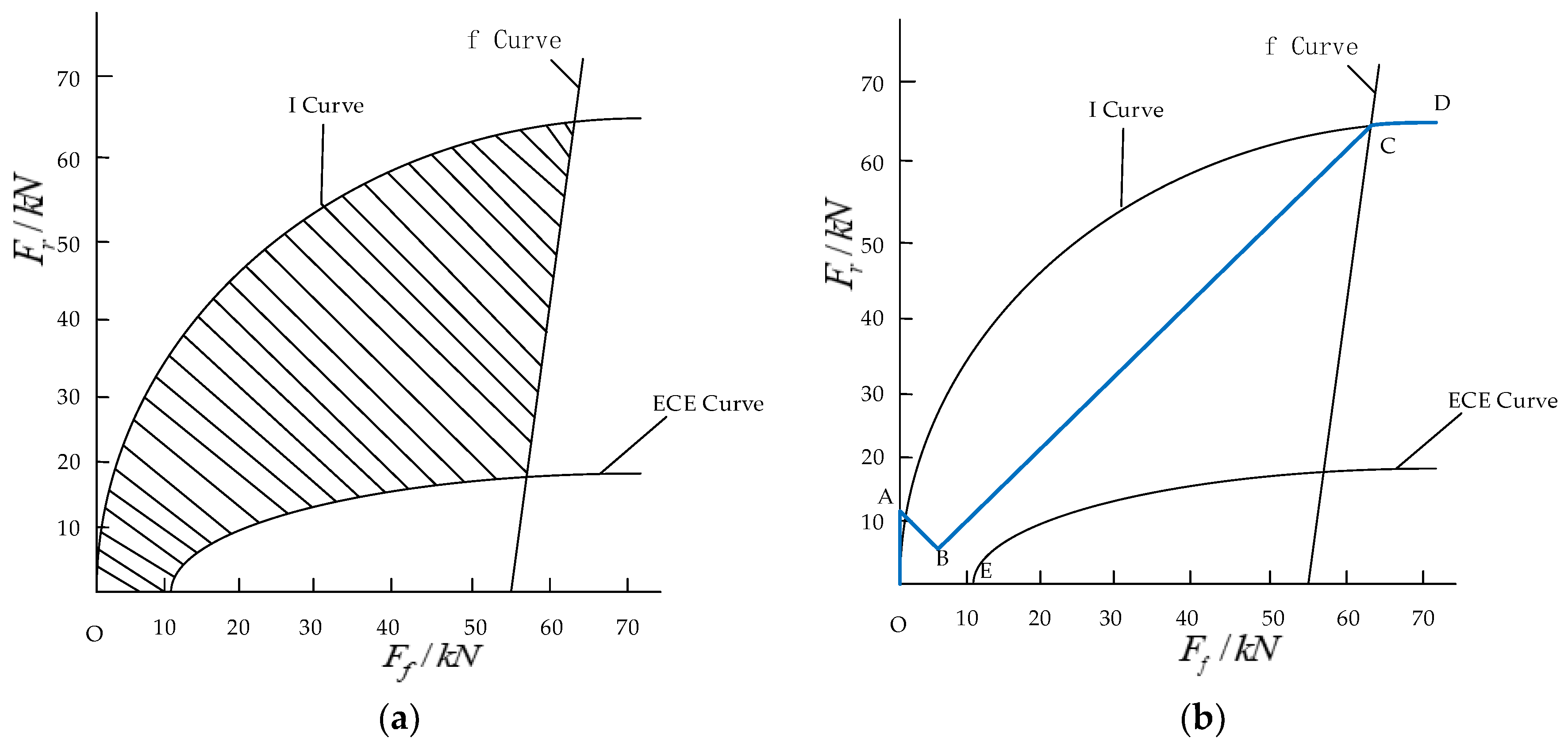
According to the analysis of the structure of the research object in this paper, there are three times the distribution of braking force: the first time, it is the distribution of braking force in the front and rear axles; the second time, it is the distribution that occurs between the motor braking and the mechanical braking; and the third time, it is the distribution of braking force between the two motors. In the process of braking force distribution, the safety of the vehicle should be ensured during braking first and secondly, as much energy as possible should be recovered. It can be concluded that the braking force distribution points of the front and rear axles should located in the area surrounded by the I curve, the ECE boundary line, the f line, and the horizontal coordinate axis, as shown in Figure 3a. The shaded area in Figure 3a is the feasible area of braking force distribution. Distributing the braking force of the front and rear axles in this area can ensure the braking stability of the vehicle and meet the regulatory requirements during braking at the same time [22].
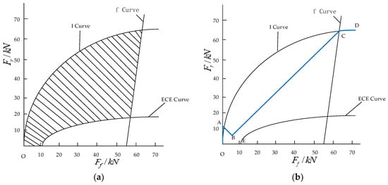
Figure 3.
(a) The feasible area of braking force distribution; (b) The braking force distribution of the front and rear axles. The point A is intersection of the line with z = 0.06 and the Y-axis; the point C is intersection of f curve and I curve; the point E is intersection of ECE curve and X-axis. The blue line OABCD is the braking force distribution curve of the front and rear axles.
In the actual braking process, the braking force of the front and rear axles is usually distributed according to a certain proportion and the closer the braking force distribution curve is to the ideal braking force distribution curve, the better safety and stability can be guaranteed during braking. Based on the above analysis of the braking force distribution of the front and rear axles, considering the constraint of the feasible region of braking force distribution of the front and rear axles, the braking force distribution of the front and rear axles is shown in Figure 3b.
The ideal braking force distribution curve in Figure 3b has an intersection point C with the f-curve with = 0.7. A braking force distribution coefficient of the front and rear axles is determined based on the intersection point C. According to the formulas of I and f curves and vehicle parameters, the coordinate of point C can be obtained as (62,009, 63,788) and the braking force distribution coefficient is calculated using Equation (1); the coefficient is calculated to be = 0.49. In Figure 3b, point E is the intersection of the ECE curve and the horizontal coordinate axis and the coordinate of point E is calculated to be (10,999, 0) and the braking strength of point E is calculated to be 0.06. At point E, make a line at 45 degrees to the negative direction of the horizontal coordinate axis and intersect the vertical coordinate axis at point A. Point B is the intersection of this line and the line with = 0.49. Via calculation, the braking strength of point C is 0.70; in order to improve the energy recovery rate during braking, according to the above analysis of braking force distribution of the front and rear axles, the OABCD curve shown in Figure 3b is the braking force distribution curve adopted in this paper [23].
In Equation (1), is the braking force of the front axis and is the braking force of the rear axis.
3.2.1. Research on the Control Strategy of the Braking Force Distribution of the Front and Rear Axles
According to the above analysis of the braking force distribution of the front and rear axles and the computational solution of every node, taking into account the braking energy recovery and braking safety, the specific braking force distribution is divided into the following three stages:
1. (OA segment). At this stage, the braking strength is very small and the braking force distribution can be unrestricted by ECE regulations. In order to maximize the rate of braking energy recovery, the rear axle bears all the braking force of the whole vehicle:
In Equation (2), is the braking force of the front axle and is the braking force of the rear axle.
2. (BC segment). Under this braking strength, the front and rear axles bear all the braking force
3. (Point C and later stage). At this time, the braking strength is large and the velocity of vehicle needs to be reduced quickly; in order to ensure the braking safety, at this time, all the braking force of the front and rear axles is provided by the mechanical braking force. The mechanical braking force of the front and rear axles is distributed according to the I-curve as follows:
In addition, considering the driving safety and comfort of the vehicle, energy recovery is not considered when the battery SOC of the vehicle is higher than the maximum recovery value and the velocity is lower than the minimum recovery value. At the moment, in order to improve the braking efficiency and braking stability, the mechanical braking force of the front and rear axles is distributed according to the I-curve. The specific allocation is shown in Equation (4).
3.2.2. Research on the Strategy of Electromechanical Braking Force Distribution of the Rear Axle
Since the motor braking force cannot always meet the demand of braking force on the rear axle, the braking force of the rear axle needs to be supplemented by part of the mechanical braking force. This involves the second distribution of the braking force. This time, the principles of braking safety and energy optimum must be followed as well.
Similarly, the distribution process of the electromechanical braking force of the rear axle is still divided into three stages:
1. (OA segment). The braking strength at this stage accounts for a considerable proportion during driving, in order to be able to recover more energy and improve the energy recovery rate, so all the braking force of the rear axle is provided by motor braking force:
In Equation (5), is the mechanical braking force of the rear axle and is the motor braking force of the rear axle.
Moreover, it is calculated that the maximum braking force required by the vehicle at this stage is less than the maximum braking force provided by the two motors. So the above distribution process can be realized.
2. (BC segment). Under this braking strength, if the braking force of the rear axle is less than the sum of the maximum braking force of the respective current speed of the dual motors, in order to improve the energy utilization rate, all the braking force of the rear axle is provided by the motor braking force. If the braking force of the rear axle is more than the sum of the maximum braking force of the respective current speed of the dual motors, the dual motors will output the maximum braking force and the rest is compensated by the mechanical braking force.
This is
In Equations (6) and (7), is the maximum braking force provided by motor 1 and is the maximum braking force provided by motor 2.
3. (Point C and later stage). Under high braking strength, in order to ensure the safety of the vehicle during braking, all the braking force of the rear axle is provided by the mechanical braking force; at this time, the motor is not involved in braking.
3.2.3. Research on the Control Strategy of Braking Force Distribution between Dual Motors
After completing braking force distribution of the front and rear axles and electromechanical braking force distribution of the rear axle, another distribution between the two motors is required. In order to further improve the energy recovery rate, a higher-efficiency motor is prioritized to brake during energy recovery.
Therefore, during the third distribution of braking force, the specific control strategy is similar to that of the driving control strategy and will not be elaborated here [24].
4. Control Strategy Based on Driver Style
Depending on the different demands of drivers for power of the vehicle, this paper classifies driver styles into three categories: The first is the radical drivers who drive roughly and need more power from the vehicle, the second is the cautious drivers who start and accelerate more slowly and pay more attention to the economy of the vehicle, and the third is the standard drivers who are between radical and cautious types.
In this paper, the correction coefficient k of the demand torque is proposed to correct the driving demand torque of the vehicle in order to obtain a more accurate demand torque that adapts different types of drivers to improve the power adaptability of the vehicle.
In Equation (8), is the actual driving demand torque of the vehicle, k is the torque correction coefficient, is a non-linear function about average acceleration, standard deviation of acceleration, accelerator pedal opening, and changing rate of accelerator pedal opening, is the maximum torque of motor 1 at speed , and is the maximum torque of motor 2 at speed .
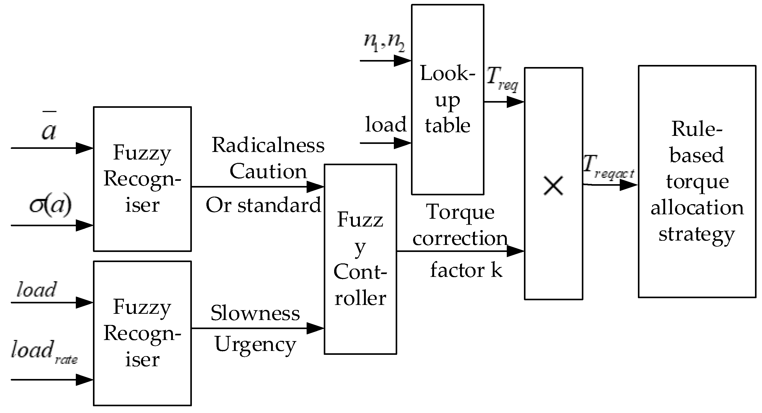
There is a non-linear relationship among the accelerator pedal opening and its changing rate, the average value of acceleration, standard deviation of acceleration and the torque correction coefficient k, and the mathematical model is difficult to determine, so a fuzzy control method is used to obtain the k value. Fuzzy identification of driver style is conducted by the average value of acceleration and standard deviation of acceleration, fuzzy identification of acceleration intention is conducted by accelerator pedal opening and the changing rate of accelerator pedal opening, and the recognition results of driver style and acceleration intention are used as two inputs to the fuzzy controller of k value to correct the driving demand torque by the k value outputted through defuzzification to obtain the demand torque that adapts driver style. The specific process of the driver style recognition is shown in Figure 4.
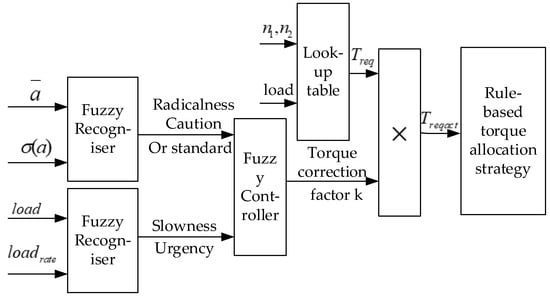
Figure 4.
The specific process of the driver style recognition.
4.1. Drivers’ Driving Style Recognition
The larger average value of acceleration may mean that the driver has a higher demand for the power of vehicles but the average value of acceleration also only reflects the average level of acceleration over a period of time, which does not reflect the dispersion degree of acceleration and therefore the standard deviation of acceleration is introduced to jointly judge the focusing type of the driver.
Considering the real-time processing capability of the hardware, this paper selects the driving cycle of the past 50 s to calculate the average value of acceleration
In Equation (9), is the ith sampling value of acceleration and n is the number of sampling.
The formula for the standard deviation of acceleration is
In Equation (10), a is the sampling value of acceleration and is the average value of acceleration.
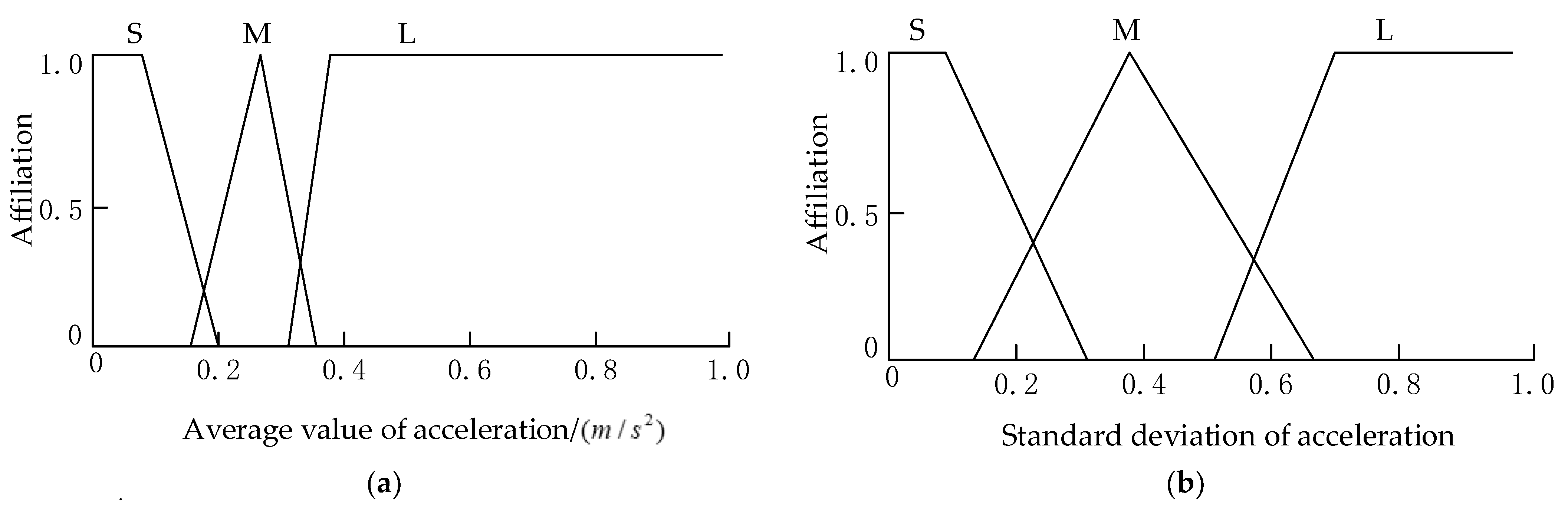
The affiliation functions of the average value of acceleration and the standard deviation of acceleration are shown in Figure 5.
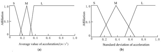
Figure 5.
(a) The affiliation function of the average value of acceleration; (b) The affiliation function of the standard deviation of acceleration. S represents small; M represents medium; L represents large.
The fuzzy inference rules of driver style recognition are shown in Table 3.
Table 3.
The fuzzy inference rules of driver style recognition.
4.2. Driver Acceleration Intention Recognition
The accelerator pedal opening reflects the urgent degree of acceleration to some extent but the accelerator pedal opening alone does not fully reflect the urgent degree of acceleration. In this paper, the accelerator pedal opening and its changing rate are selected to reflect the urgent degree of acceleration together. The acceleration of the vehicle is classified into slow acceleration and urgent acceleration. The changing rate of the accelerator pedal opening of one step has a great impact on the fluctuation of the acceleration intention of drivers, making the acceleration intention change frequently, so the average value of 50 steps is selected for the recognition of acceleration intention in this paper.
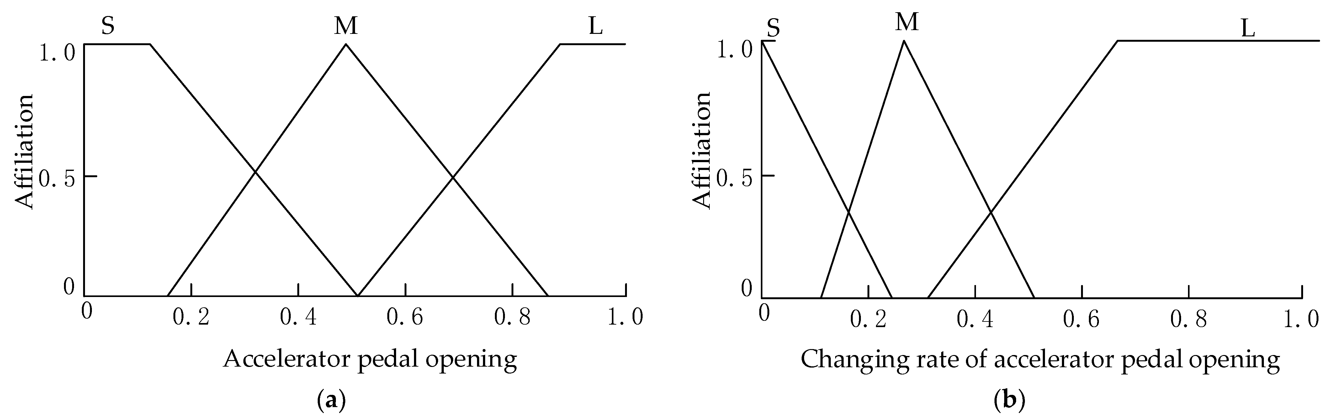
The affiliation functions of the accelerator pedal opening and the changing rate of the accelerator pedal opening are shown in Figure 6.
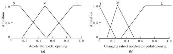
Figure 6.
(a) The affiliation function of accelerator pedal opening; (b) The affiliation function of the changing rate of accelerator pedal opening.
The fuzzy inference rules of acceleration intention are shown in Table 4.
Table 4.
The fuzzy inference rules of acceleration intention.
4.3. Driving Demand Torque Correction Coefficient k
The torque correction coefficient k is derived from the defuzzification of the fuzzy controller that takes the recognition results of driver style and acceleration intention as inputs. The driving demand torque of the vehicle is corrected by the k value to get the more accurate demand torque that adapts to the driver style so that the powertrain can work in a more reasonable working mode. The affiliation function of the torque correction coefficient is shown in Figure 7.
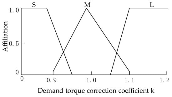
Figure 7.
The affiliation function of the torque correction coefficient.
The fuzzy inference rules of the torque correction coefficient are shown in Table 5.
Table 5.
Fuzzy inference rules of torque correction coefficient k.
4.4. Analysis of Offline Simulation
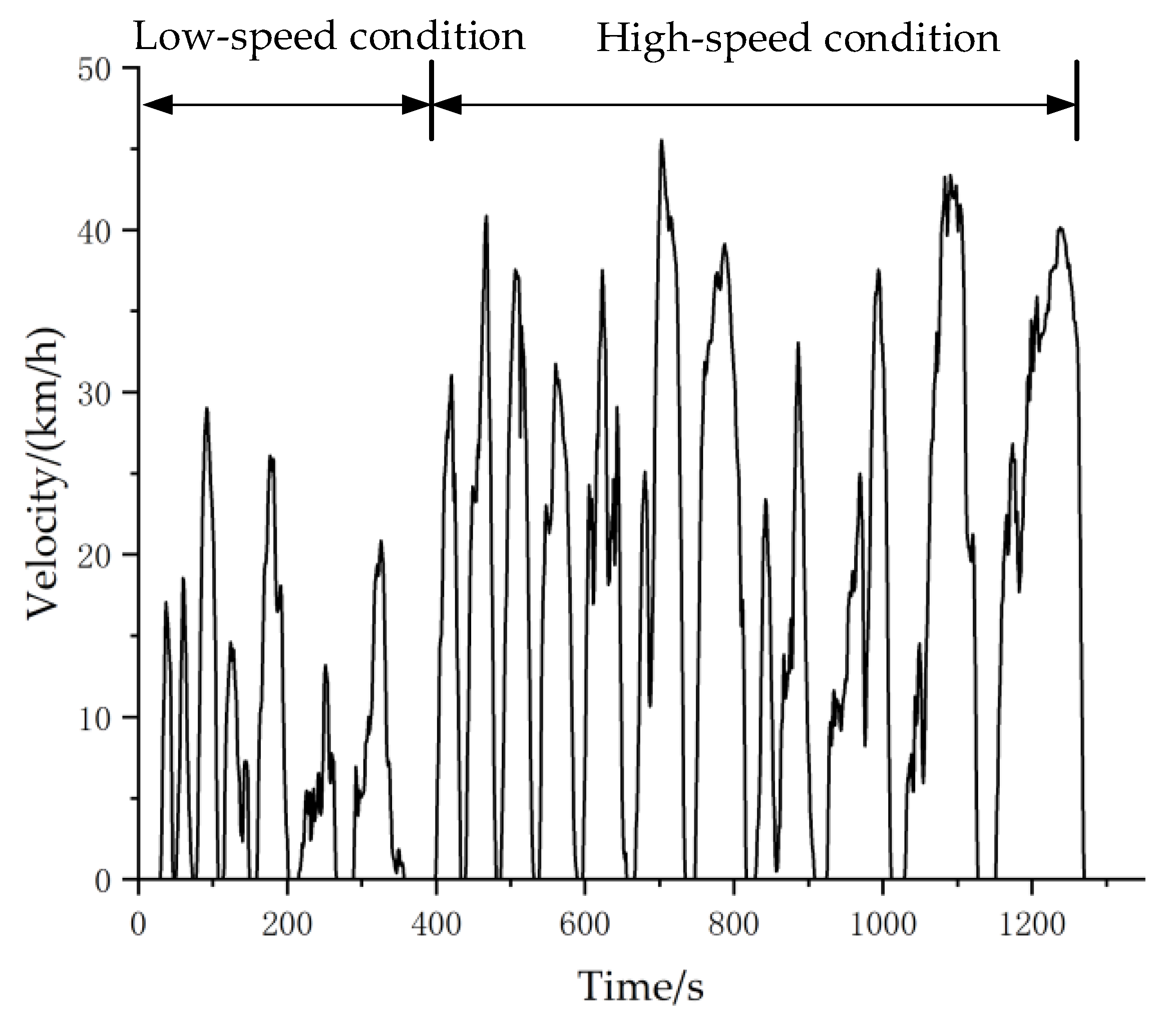
In order to make the driving cycle of simulation closer to the actual road condition, the Chinese heavy-duty commercial vehicle test cycle for the bus (CHTC-B) is selected for simulation in this paper, as shown in Figure 8.

Figure 8.
CHTC-B driving cycle.
The vehicle model is built in the CRUISE, and the control strategy is built in Simulink, and the joint simulation is carried out for the rule-based control strategy without driver style recognition and the fuzzy control strategy based on driver style, respectively.
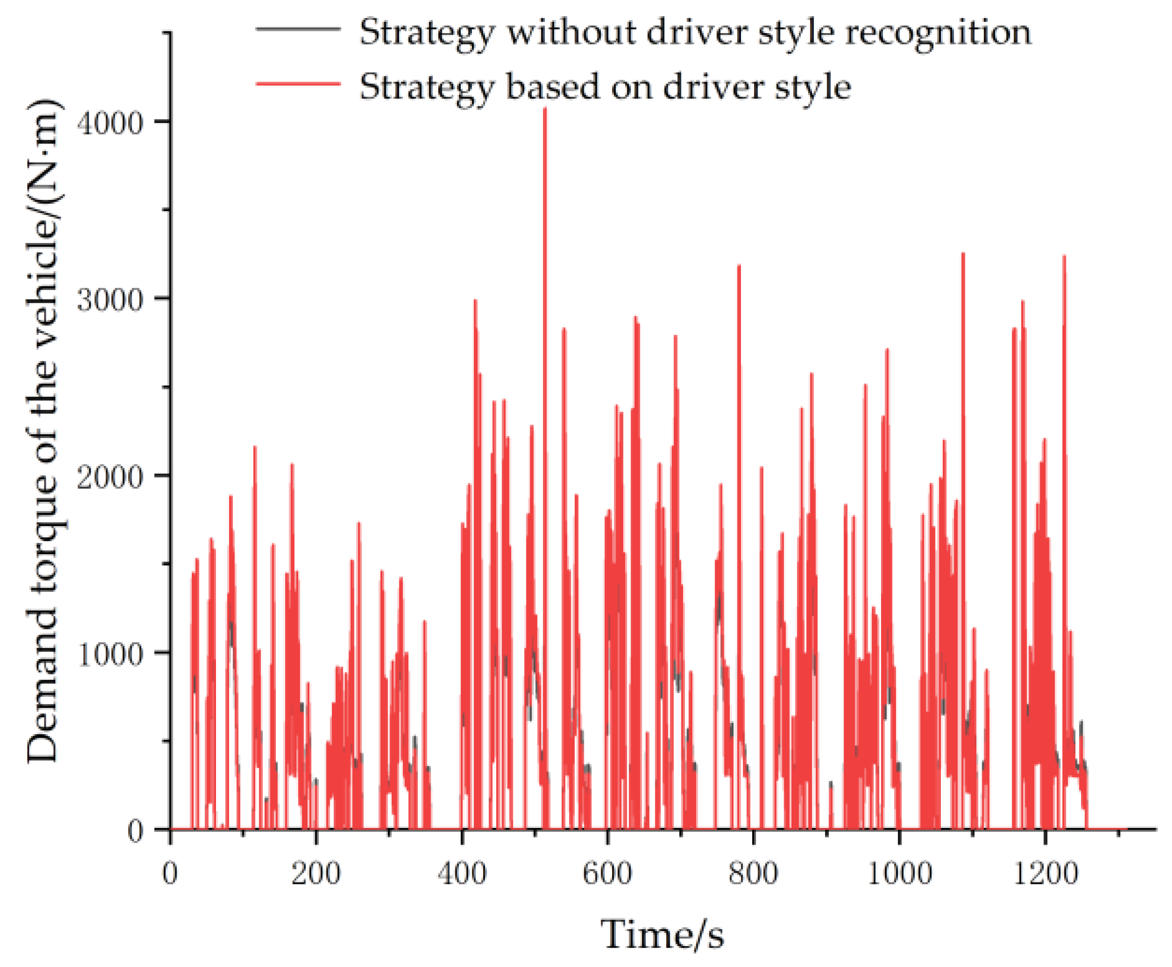
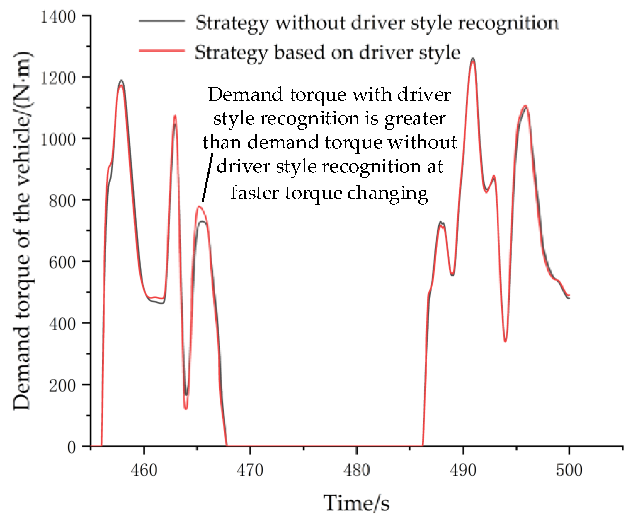
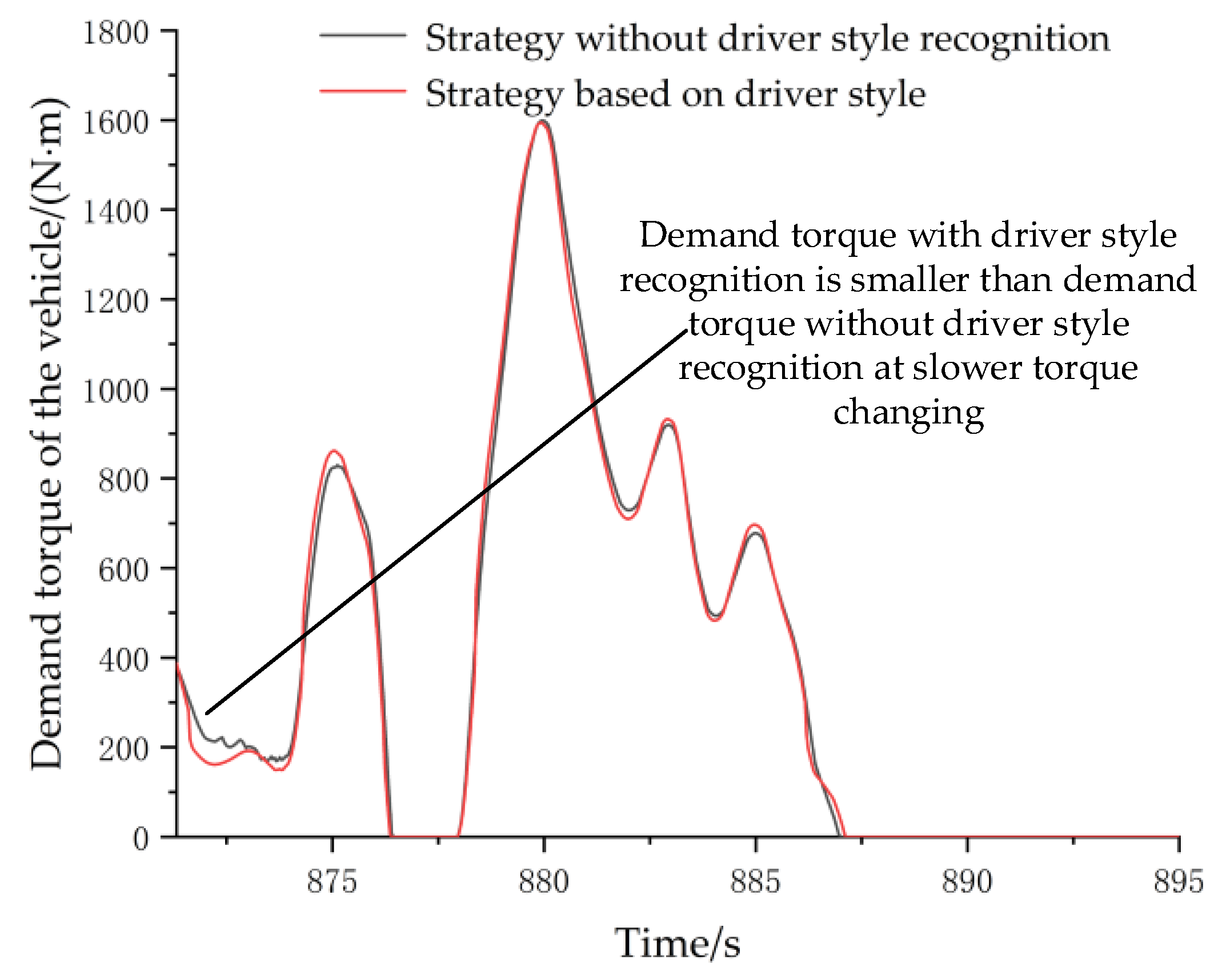
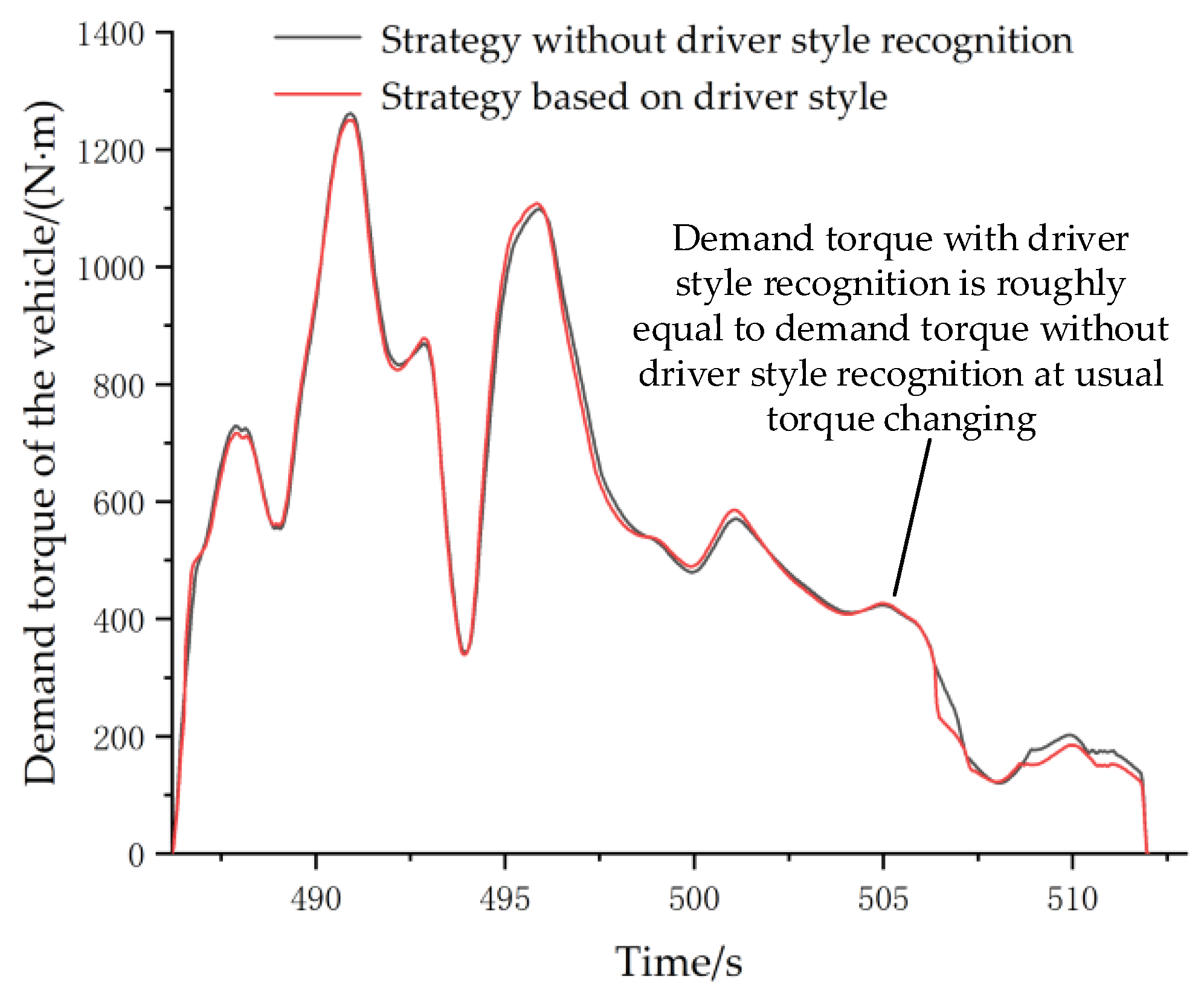
Figure 9 shows a comparison of the driving demand torque of the different strategies under the CHTC-B driving cycle. Figure 10 shows the variation in the demand torque when the driver style is radical and the outputting torque of the control strategy based on driver style is larger than that without driver style recognition when the demand torque varies largely from 464 to 466 s. Figure 11 shows the variation in the demand torque when the driver style is cautious; the outputting torque of the control strategy based on driver style is smaller than that without driver style recognition when the variation of the demand torque is small from 871 to 874 s. Figure 12 shows the variation in the demand torque when the driver style is standard and the outputting torque of the control strategy based on driver style is roughly equal to that without driver style recognition when the variation in the demand torque is usual from 501 to 506 s. This is because the driver style is recognized more accurately and the demand for the torque is more reasonable.
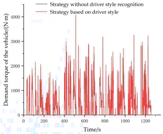
Figure 9.
Comparison of the driving demand torque of different strategies.
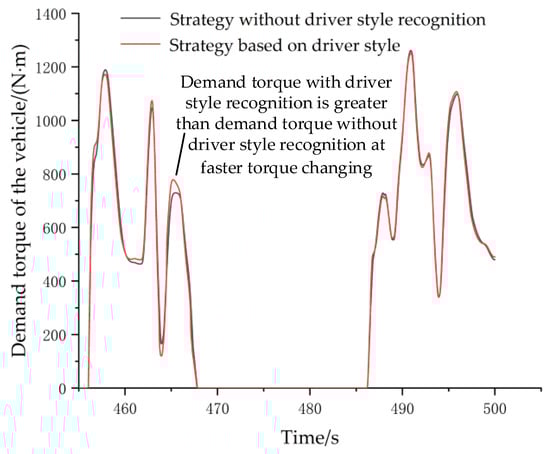
Figure 10.
Comparison of demand torque at radical type.
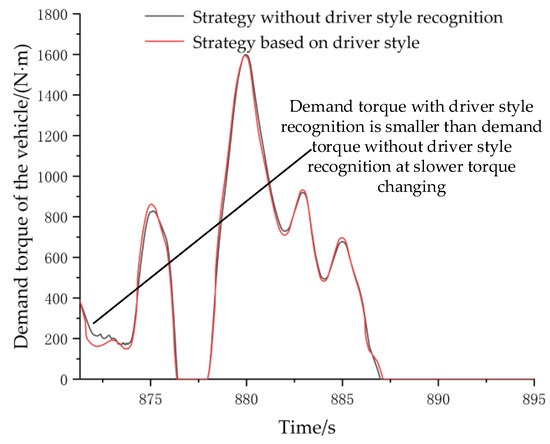
Figure 11.
Comparison of demand torque at cautious type.
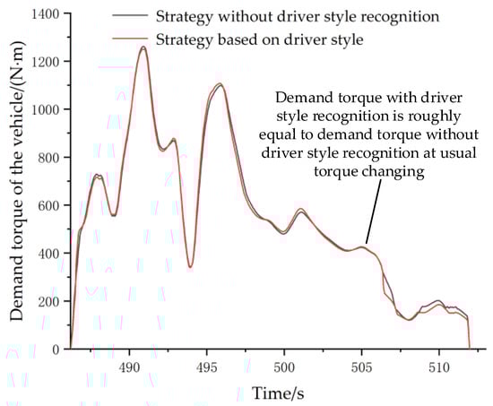
Figure 12.
Comparison of demand torque at standard type.
It can be seen that a control strategy based on driver style can adapt to different types of drivers and the power adaptation of the vehicle is improved.
5. Automatic Optimization of Parameters for the Control Strategy Based on Driver Style
The optimization of the parameters for the control strategy based on driver style is non-linear and multidirectional and the objective function to solve is just to find the optimal solution in the feasible domain of the control variables under the condition of meeting the constraints so that the economy of the vehicle can be further improved.
5.1. Build Optimization Model
The optimization problem of control strategy based on driver style can be stated as a constrained nonlinear optimization problem and the mathematical model is
In Equation (11), is the optimization objective function, is the 100-kilometre electricity consumption of the vehicle, is the jth constraint about the variable x, m is the number of constraints, and are the lower and upper limit of the ith optimization variable , respectively, and n is the number of optimization variables.
5.1.1. Establish Optimization Goal
In this paper, the model is an electric vehicle and the design objective is to achieve the optimal economy under the premise of meeting the dynamics, so the optimization objective is the power consumption of 100 km of the vehicle.
5.1.2. Restrictive Condition
Constraints of the electric vehicle are dynamic performance indicators and tracking errors of the driving cycle path. The specific constraint indicators are shown in Table 6.
Table 6.
Constraint conditions.
5.1.3. Selection of Optimization Variables
Based on the analysis of the above strategy, the optimization of some of the parameters selected in the strategy that have a greater impact on the vehicle economy is carried out. Optimization variables selected in the control strategy are correction coefficients m and n of the velocity logic threshold values of selecting the higher-efficiency motors 1 and 2 when acting in first gear in the driving control strategy and correction coefficients x and y of the velocity logic threshold value of selecting the higher-efficiency motors 1 and 2 when acting in second gear in this strategy. The optimization variables are selected as shown in Table 7.
Table 7.
Selection process of the optimization variables.
The reason for the parameter selection is mainly that the high-efficiency range of the motor we visually measured according to the efficiency map of the motor is not the optimal range, so the resulting velocity range and the velocity logic threshold values of selecting the higher-efficiency motor are also not optimal. Therefore, the velocity logic threshold values need to be corrected to make them optimal to achieve the purpose of improving the efficiency of the vehicle and reducing energy consumption.
5.2. Selection of Optimization Algorithms
In this paper, Multi-Island Genetic Algorithm (MIGA) and Non-Linear Sequential Quadratic Programming (NLSQP) are selected to optimize parameters.
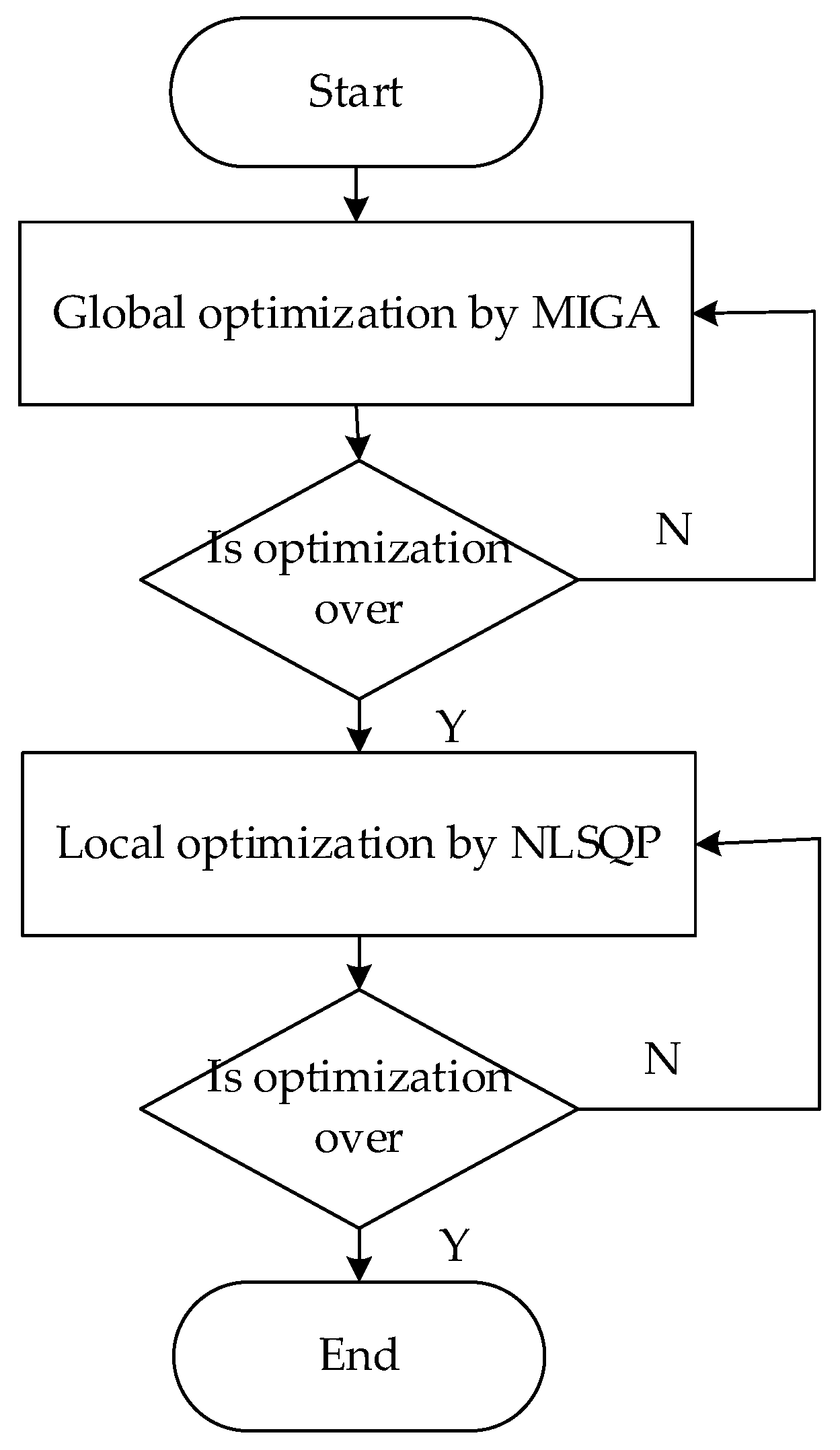
In the early stage of the optimization process, the global optimization ability of MIGA is utilized to locate the global optimal region initially and, in the later stage of the optimization process, the local optimization ability of NLSQP is utilized to quickly search for the optimal solution in the optimal region to improve the speed of the optimization and achieve the rapid search for the global optimal solution, which not only improves the efficiency of optimization but also improves the quality of optimization. The process of the combined optimization is shown in Figure 13.
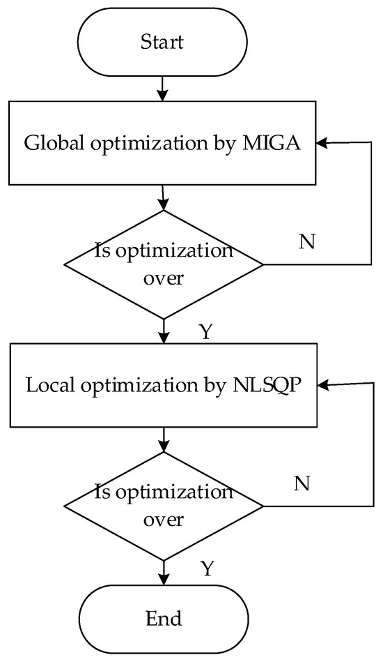
Figure 13.
The process of the combined optimization. Y represents yes; N represents no.
5.3. The Development of the Isight Optimization Platform
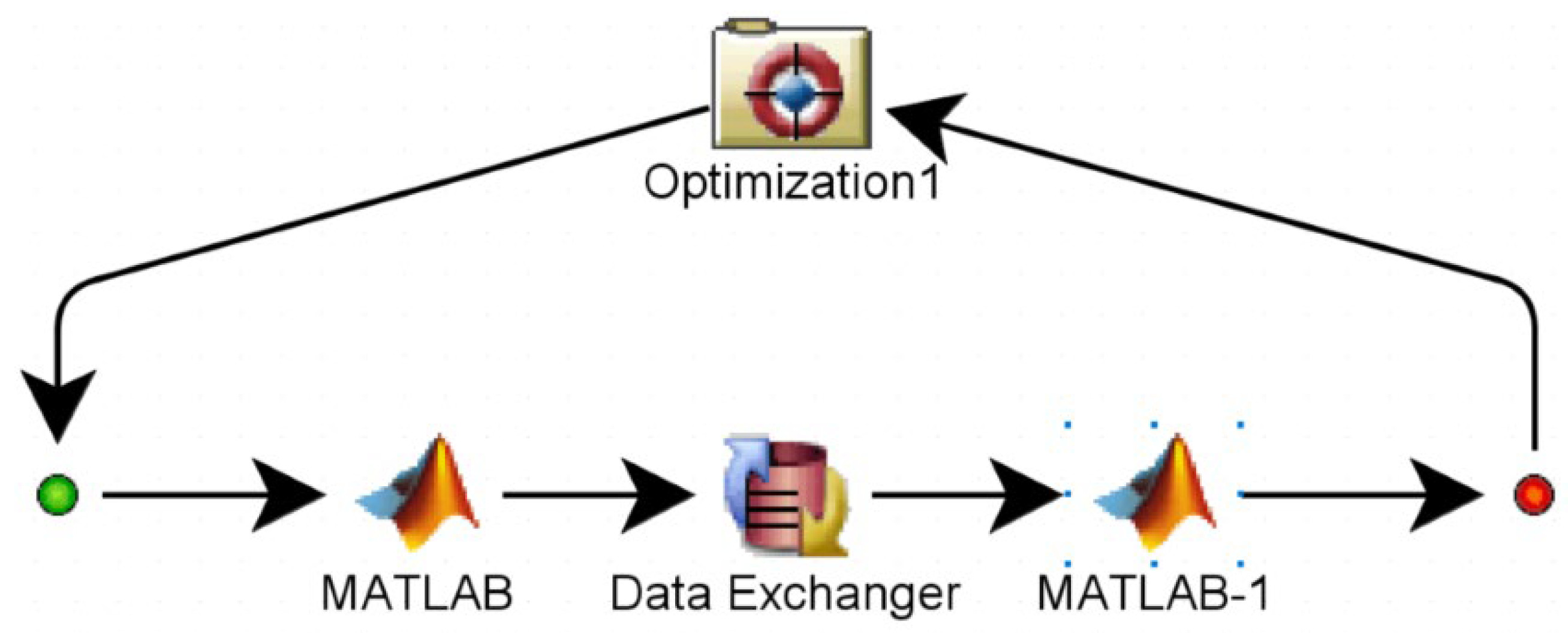
The Isight optimization platform is shown in Figure 14. The combined algorithm of the Multi-Island Genetic Algorithm and Nonlinear Sequential Quadratic Programming is selected to optimize the control parameters and set the range of parameters, limiting values and so on in Optimization1 component. The inputs (i.e., the four optimization variables) are selected and the parameter calibration program and simulation interface startup program are written in the Matlab component. The location and content of the data in the Data Exchanger component are determined and a data processing program in the Matlab1 component to obtain the constraint values is written, which are passed to the optimization algorithm set up in the Optimization1 component. The optimization is carried out automatically until the maximum number of iterations is reached and the optimal control parameters and optimization object are output.
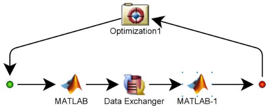
Figure 14.
Isight optimization platform. Matlab: co-simulation of Simulink and Cruise; Data Exchanger: acquire test data; Matlab1: calculate optimization result.
6. The Result and Analysis of Optimization Simulation
6.1. Analysis of Optimization Results
The Chinese city bus driving cycles (CHTC-B) in Cruise are loaded and the Isight optimization platform for automatic optimization is started; the process of optimization is shown in Figure 15. From the figure, it can be seen that the optimal solution occurs in generation 594; at this time, the power consumption per 100 km is 83.77 kW h and the economy is improved by 2.16% compared to the pre-optimization. The comparison results of the control parameters before and after optimization are shown in Table 8.
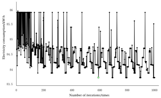
Figure 15.
Optimization process of the automatic optimization platform. The green dot represents the optimum optimization goal during automatic optimization.
Table 8.
Comparison of parameters before and after optimization.
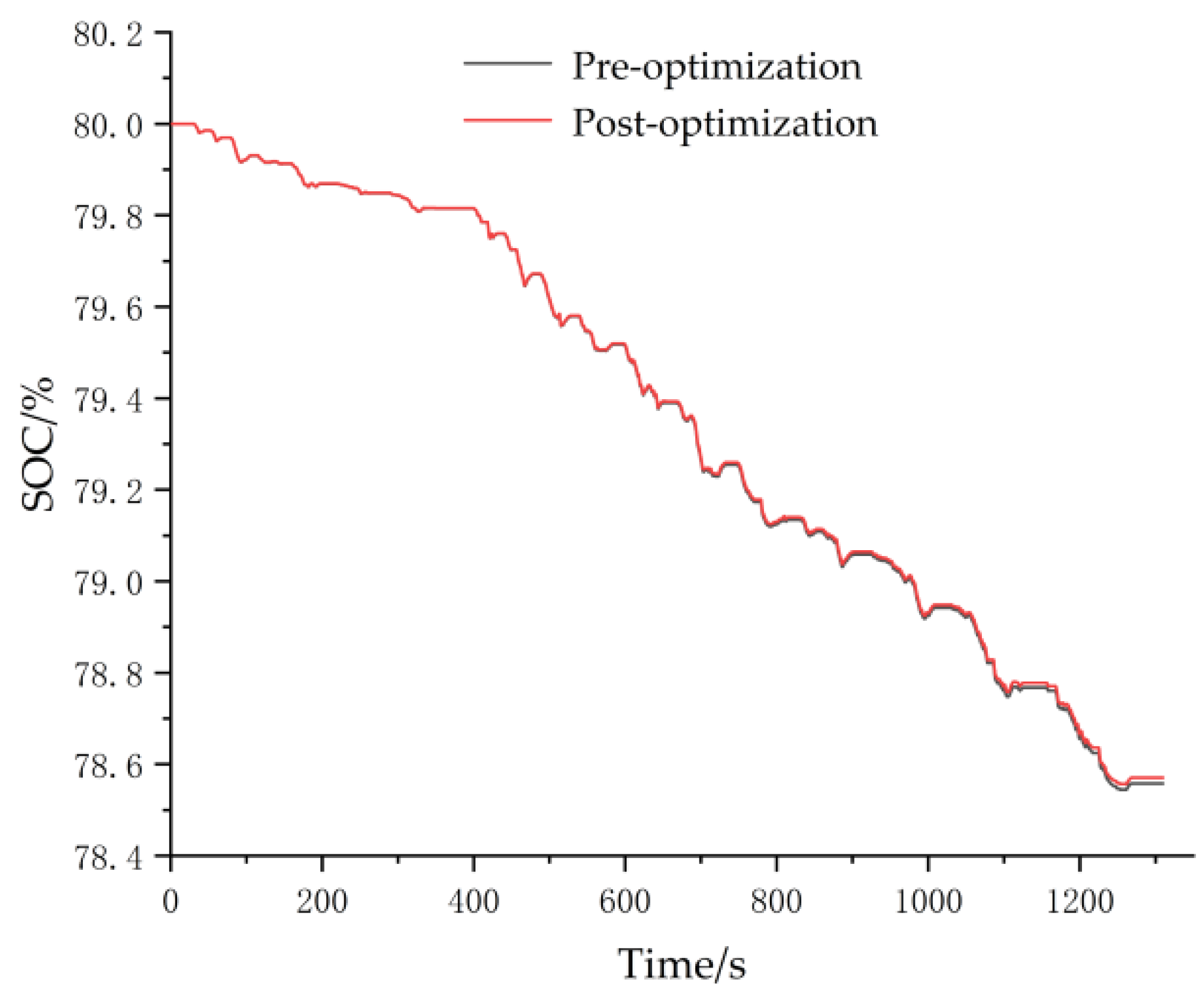
The changing curves of battery SOC before and after optimization are shown in Figure 16. With regard to Figure 16, after optimization, the changing of battery SOC is smoother, avoiding rapid discharge to a certain extent, which is conducive to prolonging the driving miles and battery service life [25].
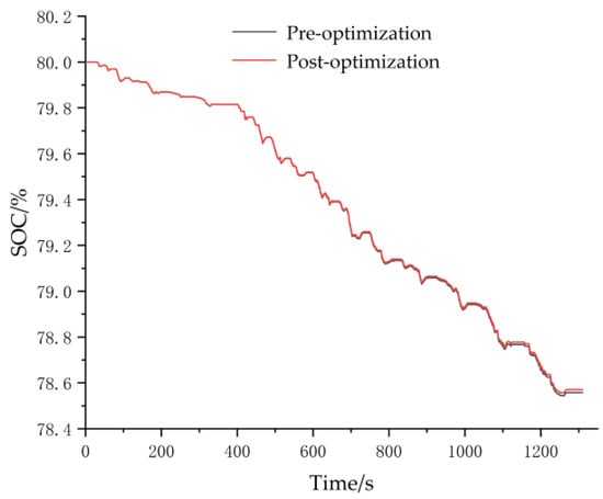
Figure 16.
Comparison of battery SOC.
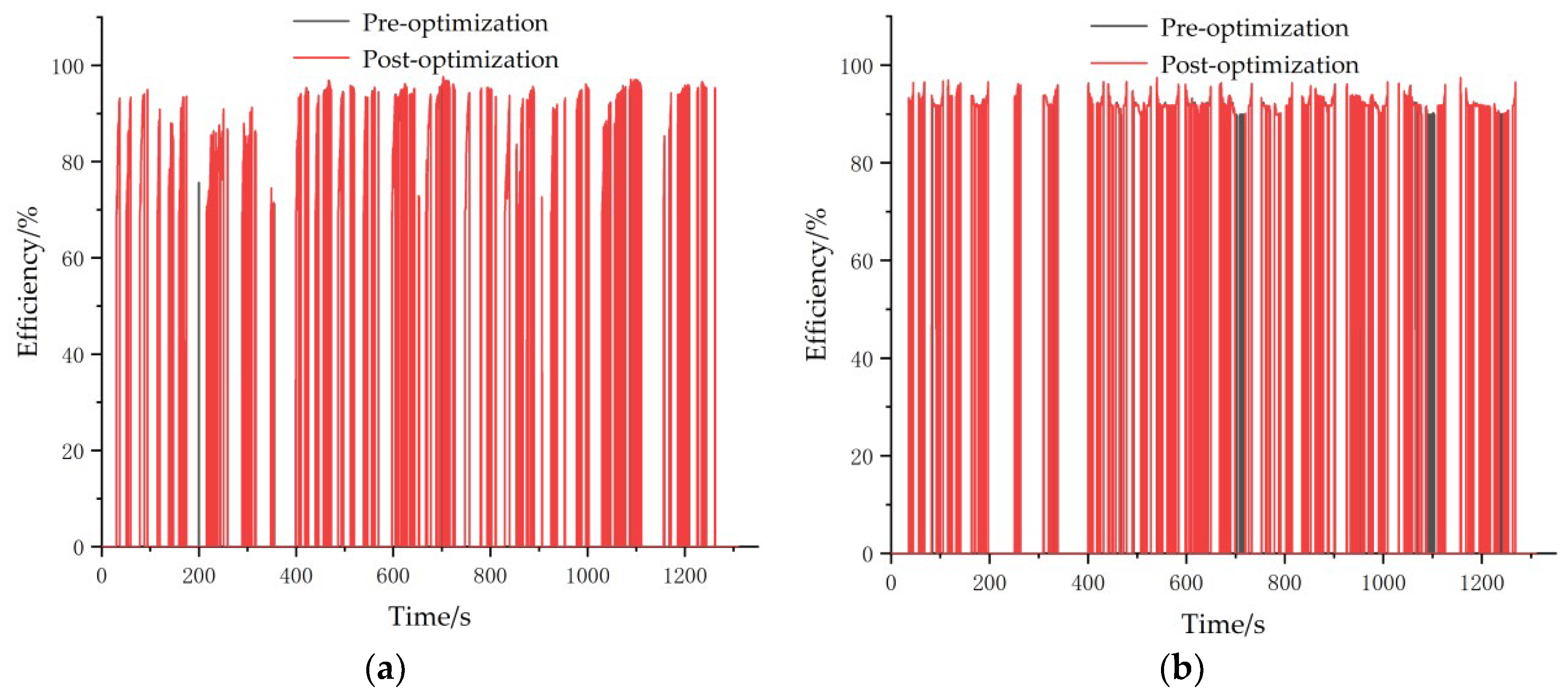
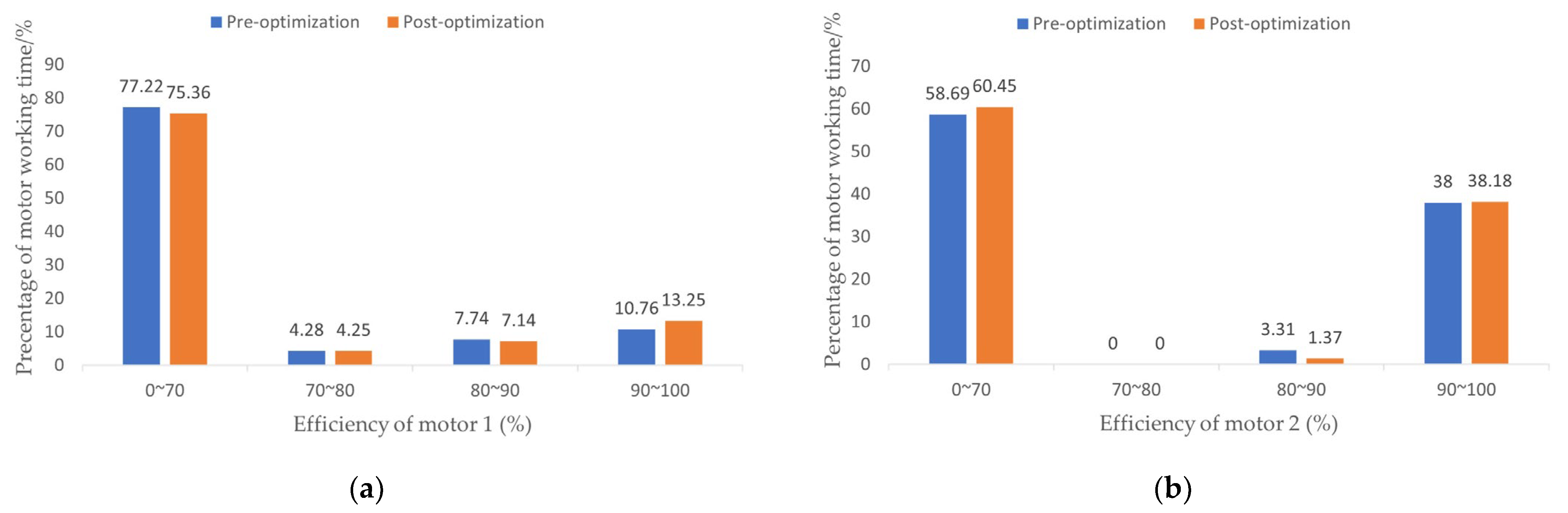
In order to analyze the results before and after optimization in more detail, a comparison of the efficiency for motor 1 and motor 2 under the CHTC-B driving cycle before and after optimization is shown in Figure 17. The corresponding percentage of the working efficiency of motors 1 and 2 before and after optimization is shown in Figure 18.
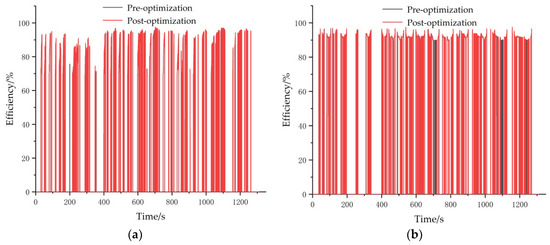
Figure 17.
(a) Comparison of efficiency for motor 1; (b) Comparison of efficiency for motor 2.
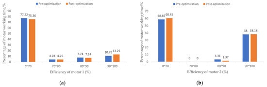
Figure 18.
(a) Comparison of percentage of working efficiency of the motor 1; (b) Comparison of percentage of working efficiency of the motor 2.
From Figure 18a,b, it can be seen that after optimization, the operation time percentage of the efficiency zone is greater than 90% (i.e., high-efficiency working zone) of motor 1 and 2 is improved by 2.67%; however, there is a decrease in operation time percentage of the efficiency zone of less than 70% (i.e., low-efficiency working zone). So, after optimization, the working efficiency of the motors 1 and 2 is further improved compared to pre-optimization and the purpose of improving the economy is achieved.
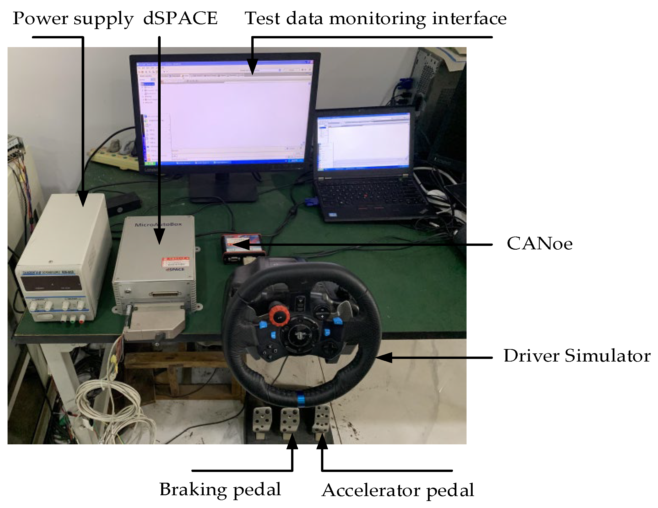
6.2. Semi-Physical Simulation Test Verification
The semi-physical simulation test platform mainly consists of a hardware system (dSPACE, CANoe, driver simulator), software system (AVL_Cruise, Matlab, data monitoring software Control Desk V7.6.1), etc. The optimized strategy based on driver style is compiled and downloaded into dSPACE and through the built-in digital-to-analog conversion channel of dSPACE, the accelerator pedal signal and braking pedal signal are converted into digital signal. CANoe is the CAN communication controller, which realizes the communication of the whole vehicle by accepting and sending data. The driver simulator can realize the human—machine interaction in hardware-in-the-loop and the driver can better simulate the real driving situation by tracking the target velocity. The interface configuration is completed in Matlab/Simulink and the vehicle model is built in the AVL_Cruise. The optimized strategy based on driver style is verified by a semi-physical test. In the problem of real-time, the fuzzy controller is transformed into the corresponding fuzzy query table. The semi-physical test platform is shown in Figure 19.

Figure 19.
Semi-physical simulation test platform.
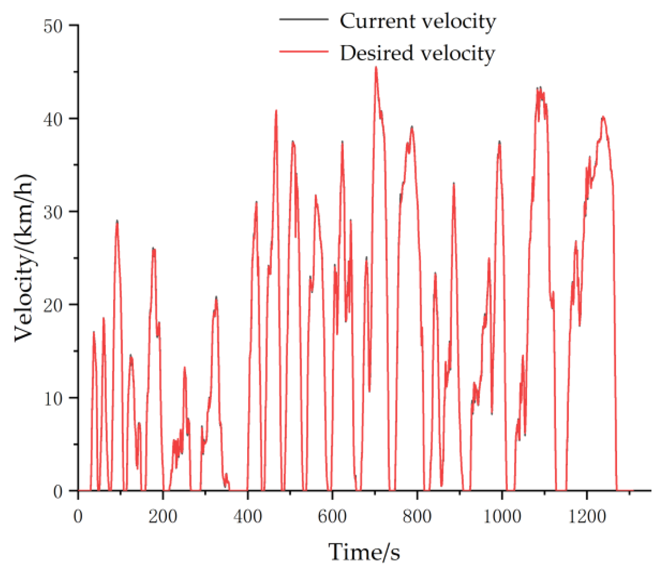
Figure 20 represents the changing curve of velocity tracing, from which it can be seen that the driver accomplished the tracing of velocity well, indicating that when the semi-physical test is carried out, it meets the dynamic performance requirements of the vehicle.
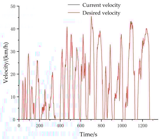
Figure 20.
Comparison of current velocity and desired velocity.
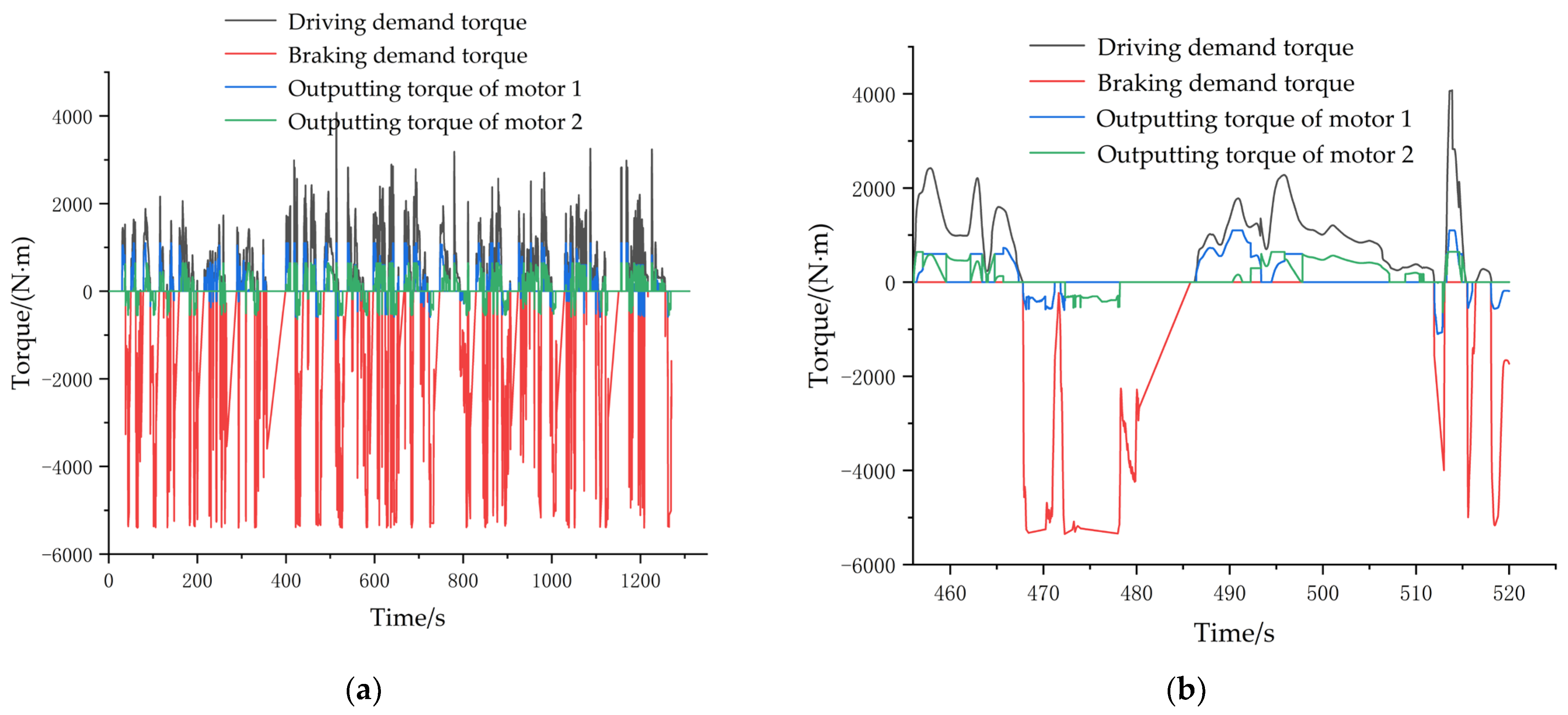
Figure 21a shows the relationship among the driving demand torque, braking demand torque and the outputting torque of motor 1 and 2 in the semi-physical test, in which 456~520 s are intercepted, as shown in Figure 21b, from which it can be seen that the driving demand torque is well allocated between motor 1 and 2 and that at higher braking strength, braking demand torque may require mechanical braking torque in addition to the motor braking torque.
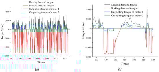
Figure 21.
(a) The torque distribution after optimization; (b) The specific torque distribution between 456~520 s after optimization.
Table 9 shows a comparison of the results of power consumption between the semi-physical test and the offline optimization. As can be seen from Table 9, the results of power consumption per 100 km of the semi-physical test and offline optimization are basically the same, thus verifying the accuracy and effectiveness of the optimized strategy based on driver style.
Table 9.
Results comparison of the semi-physical test and off-line optimization.
7. Discussion
At present, most strategies cannot adapt the driving styles of drivers; parameter optimization of the strategy was debugged manually, which was time-consuming and easy to miss the optimal solution.
To solve the above problem, a driver style recognition model based on fuzzy control method is added the rule-based control strategy to obtain a more accurate driving demand torque that adapts the driving styles of drivers. Simulation results show that control strategy based on driver style can adapt different types of drivers, improving the power adaptation of the vehicle. Automatic optimization of the control parameters in the strategy based on driver style is performed to determine the optimal control parameters and calibrate them for the purpose of improving the economy. The simulation results show that after optimization, operation time percentage of efficiency zone greater than 90% (i.e., a high-efficiency working zone) of motor 1 and 2 is improved by 2.67%; however, there is a decrease in operation time percentage of the efficiency zone of less than 70% (i.e., low-efficiency working zone). Finally, the optimized strategy is verified by a semi-physical test: the power consumption per 100 km of the semi-physical test and offline optimization is basically the same, which are 83.86 kW h and 83.77 kW h, respectively. Compared with the pre-optimization, the economy is improved by 2.06% and 2.16%.
8. Conclusions
In order to improve the overall performance of the vehicle, a driving control strategy based on the principle of prioritizing a high-efficiency motor and a braking control strategy of the distribution of multilevel braking force are firstly formulated. Then, to make the strategy adapt driving styles of drivers, a driver style recognition model based on fuzzy control method is added the rule-based control strategy; driving demand torque is corrected by a k value outputted through defuzzification to obtain a more accurate demand torque that adapts driving styles of drivers, improving the power adaptation of the vehicle. Finally, in order to further improve the economy of the vehicle, the strategy based on driver style is automatically optimized by an Isight optimization platform to make the strategy reach optimum.
The simulation results show that the strategy based on driver style can adapt to the torque demand of different types of drivers, improving the power adaptation of the vehicle; the economy of the vehicle is improved by 2.16% compared with pre-optimization. The relative error of the result of between the semi-physical test and the off-line optimization is only 0.10%, which verifies the effectiveness and reasonability of the optimized strategy.
Author Contributions
Conceptualization, G.S.; methodology, G.S.; software, G.S.; validation, G.S.; data curation, G.S.; writing—original draft preparation, G.S.; writing—review and editing, G.S. and J.X.; visualization, G.S. and J.X.; supervision, J.X. and J.G.; project administration, J.X.; funding acquisition, J.G. All authors have read and agreed to the published version of the manuscript.
Funding
This research was funded by Central Plains technological innovation leading talents, grant number [224200510014], and the APC was funded by [224200510014].
Data Availability Statement
The original contributions presented in the study are included in the article, further inquiries can be directed to the corresponding author/s.
Conflicts of Interest
The authors declare no conflicts of interest.
References
- Bonsu, N.O. Towards a Circular and Low-Carbon Economy: Insights from the Transitioning to Electric Vehicles and Net Zero Economy. J. Clean. Prod. 2020, 256, 120659. [Google Scholar] [CrossRef]
- Lv, C.; Liu, Y.; Hu, X.; Guo, D.; Wang, F.Y. Simultaneous Observation of Hybrid States for Cyber-Physical Systems: A Case Study of Electric Vehicle Powertrain. IEEE Trans. Cybern. 2018, 48, 2357–2367. [Google Scholar] [PubMed]
- Qi, J.; Liu, L.; Shen, Z.; Xu, B.; Leung, K.S.; Sun, Y. Low-Carbon Community Adaptive Energy Management Optimization toward Smart Services. IEEE Trans. Ind. Inform. 2019, 16, 3587–3596. [Google Scholar] [CrossRef]
- Li, Z.; Khajepour, A.; Song, J. A Comprehensive Review of the Key Technologies for Pure Electric Vehicles. Energy 2019, 182, 824–839. [Google Scholar] [CrossRef]
- Chopra, S.; Bauer, P. Driving Range Extension of EV With On-Road Contactless Power Transfer—A Case Study. IEEE Trans. Indust. Electron. 2013, 60, 329–338. [Google Scholar] [CrossRef]
- Meilan, Z.; Jifeng, F.; Yu, Z. Research on Power Allocation Control Strategy for Compound Electric Energy Storage System of Pure Electric Bus. Trans. China Electrotech. Soc. 2019, 34, 5001–5013. [Google Scholar]
- Meilan, Z.; Jifeng, F.; Yu, Z. Composite Energy Storage System and Its Energy Control Strategy for Electric Vehicles. Electr. Mach. Control. 2019, 23, 51–59. [Google Scholar]
- Hu, J.J.; Zu, G.Q.; Jia, M.X. Parameter Matching and Optimal Energy Management for a Novel dual-motor multi-modes Powertrain System. Mech. Syst. Signal Process. 2019, 116, 113–128. [Google Scholar] [CrossRef]
- Zhang, S.; Zhang, C.N.; Han, G.W. Optimal Control Strategy Design based on Dynamic Programming for a Dual-Motor Coupling-Propulsion System. Sci. World J. 2014, 2014, 958239. [Google Scholar] [CrossRef] [PubMed]
- Wang, Z.P.; Wang, Y.C.; Zhang, L. Vehicle Stability Enhancement through Hierarchical Control for a Four-Wheel-Independently-Actuated Electric Vehicle. Energies 2017, 10, 947. [Google Scholar] [CrossRef]
- Lian, J.; Li, L.H.; Liu, X.Z.; Huang, H.; Zhou, Y.; Han, H. Research on Adaptive Control Strategy Optimization of Hybrid Electric Vehicle. J. Intell. Fuzzy Syst. 2016, 30, 2581–2592. [Google Scholar] [CrossRef]
- Kim, J. Optimal Power Distribution of Front and Rear Motors for Minimizing Energy Consumption of 4-wheel-drive Electric Vehicles. Int. J. Automot. Technol. 2016, 17, 319–326. [Google Scholar] [CrossRef]
- Yang, Y.; He, Q.; Chen, Y.; Fu, C. Efficiency Optimization and Control Strategy of Regenerative Braking System with Dual Motor. Energies 2020, 13, 711. [Google Scholar] [CrossRef]
- Li, S.; Yu, B.; Feng, X. Research on Braking Energy Recovery Strategy of Electric Vehicle based on ECE Regulation and I Curve. Sci. Prog. 2020, 103, 0036850419877762. [Google Scholar] [CrossRef] [PubMed]
- Khayyam, H.; Bab-Hadiashar, A. Adaptive Intelligent Energy Management System of Plug-in Hybrid Electric Vehicle. Energy 2014, 69, 319–335. [Google Scholar] [CrossRef]
- Gao, J.; Zhao, J.; Yang, S.; Xi, J. Control Strategy of Plug-in Hybrid Electric Bus based on Driver Intention. J. Mech. Eng. 2016, 52, 107–114. [Google Scholar] [CrossRef]
- Qin, D. Dynamic Drive Control Strategy for Pure Electric Vehicle based on Driver Intention Recognition. Automot. Eng. 2015, 37, 26–32. [Google Scholar]
- Wang, H.; Wu, H. Implementation of an Energy Management Strategy with Drivability Constraints for a Dual-Motor Electric Vehicle. World Electr. Veh. J. 2019, 10, 28. [Google Scholar] [CrossRef]
- Liu, W.; Bi, S.; Xu, C. Shifting Strategy for Two-speed AMT of Electric Vehicle. J. Chongqing Inst. Technol. (Nat. Sci.) 2021, 35, 41–49. [Google Scholar]
- Koch, A.; Burchner, T.; Herrmann, T.; Lienkamp, M. Eco-driving for different electric powertrain topologies considering motor efficiency. World Electr. Veh. J. 2021, 12, 6. [Google Scholar] [CrossRef]
- Liu, T.; Tan, W.; Tang, X.; Zhang, J.; Xing, Y.; Cao, D. Driving conditions-driven energy management strategies for hybrid electric vehicles: A review. Renew. Sustain. Energy Rev. 2021, 151, 111521. [Google Scholar] [CrossRef]
- He, H.; Lou, J. Research on Single Pedal Regenerative Braking Control. Veh. Power Technol. 2022, 2, 1–6. [Google Scholar]
- Zhang, Z.; Dong, Y.; Han, Y. Dynamic and Control of Electric Vehicle in Regenerative Braking for Driving Safety and Energy Conservation. J. Vib. Eng. Technol. 2020, 8, 179–197. [Google Scholar] [CrossRef]
- Wang, Z.; Zang, L.G.; Jiao, J.; Mao, Y.L. Research on Hierarchical Control Strategy of Automatic Emergency Braking System. World Electr. Veh. J. 2023, 14, 97. [Google Scholar] [CrossRef]
- Li, Z.Y. Energy Recovery of Electric Vehicle Base on NEDC Cycle. Automob. Appl. Technol. 2021, 46, 1–4. [Google Scholar]


Disclaimer/Publisher’s Note: The statements, opinions and data contained in all publications are solely those of the individual author(s) and contributor(s) and not of MDPI and/or the editor(s). MDPI and/or the editor(s) disclaim responsibility for any injury to people or property resulting from any ideas, methods, instructions or products referred to in the content. |
© 2024 by the authors. Licensee MDPI, Basel, Switzerland. This article is an open access article distributed under the terms and conditions of the Creative Commons Attribution (CC BY) license (https://creativecommons.org/licenses/by/4.0/).