
Remote Sensing Identification and Stability Change of Alpine Grasslands in Guoluo Tibetan Autonomous Prefecture, China

Abstract
:1. Introduction
2. Materials and Methods
2.1. Study Area
2.2. Data and Preprocessing
2.3. Method and Process
2.3.1. Random Forest Classification
2.3.2. Precision Evaluation
2.3.3. Grassland Quality Division
2.3.4. Stability Analysis of Alpine Grassland
3. Results
3.1. Grass Extraction Accuracy
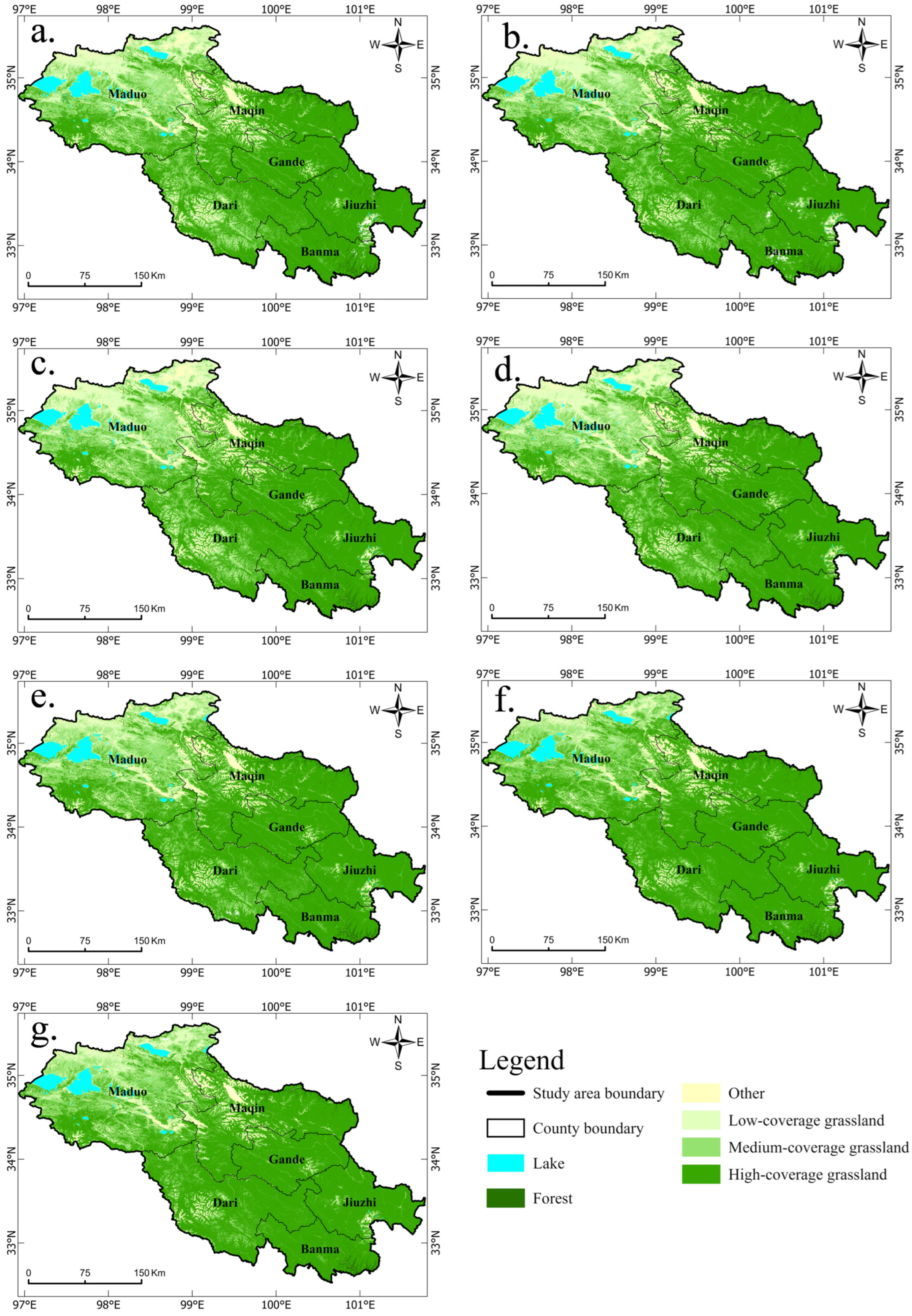
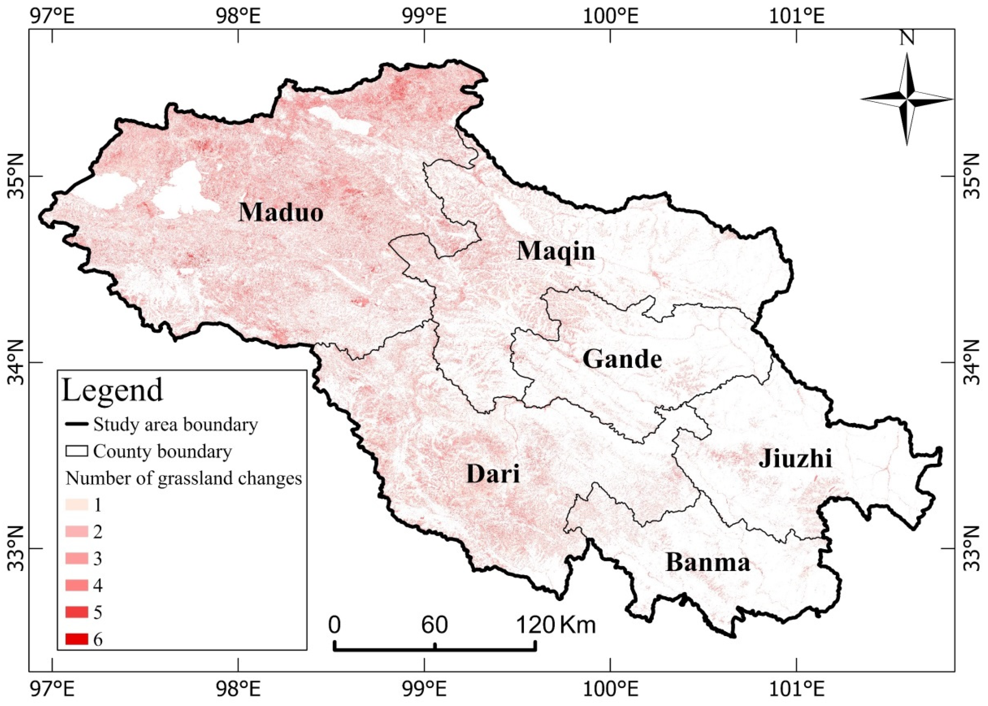
3.2. Grassland Spatiotemporal Distribution and Change
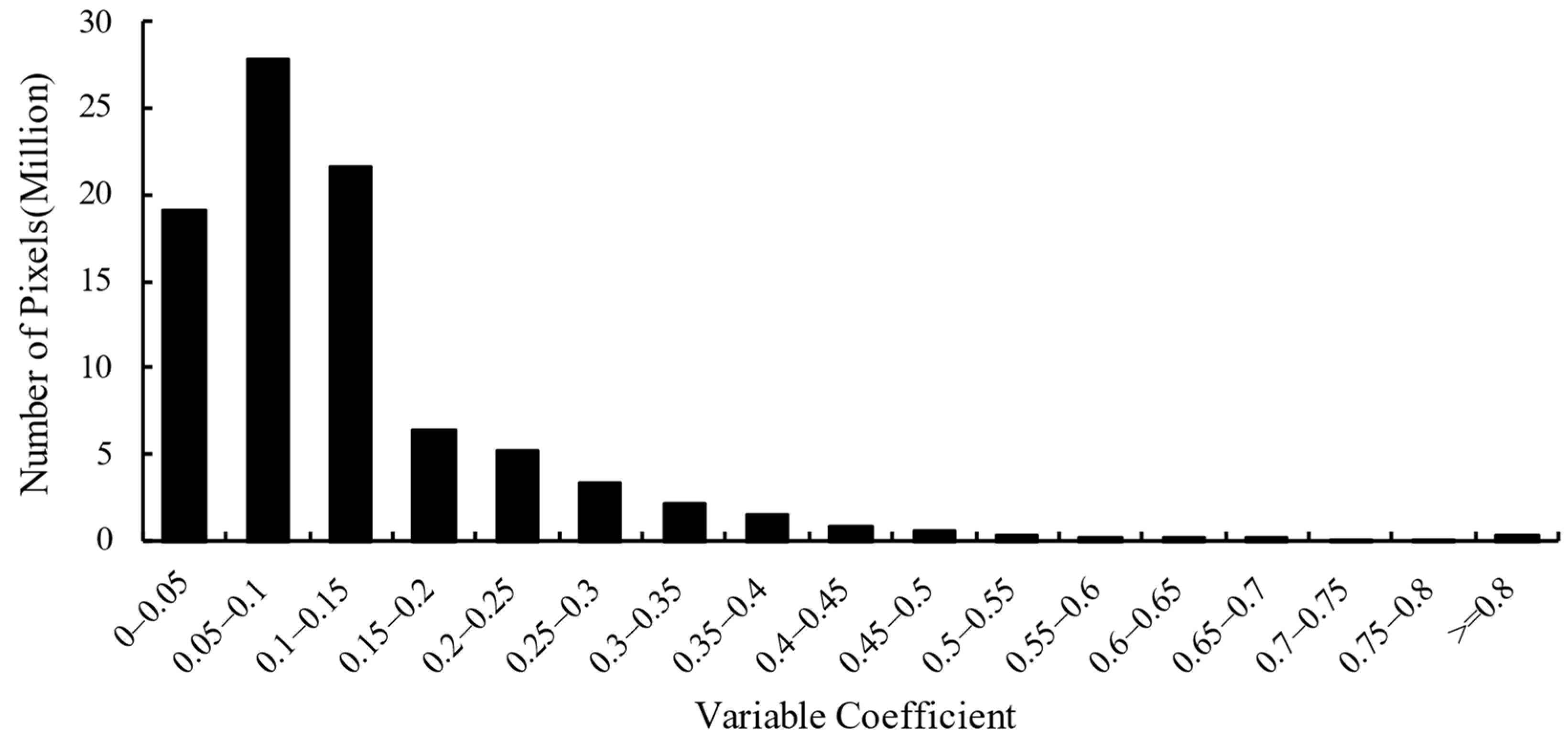
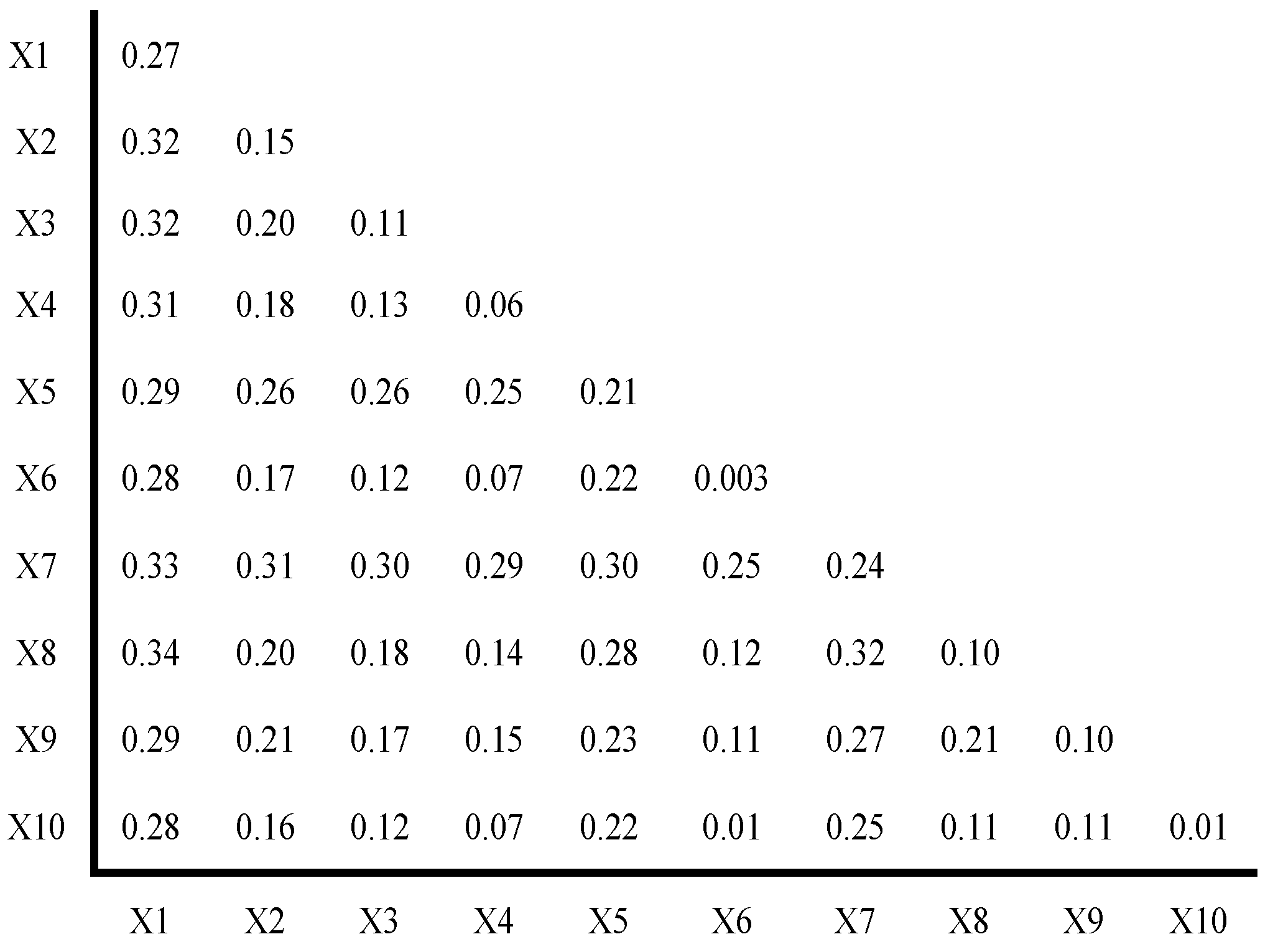
3.3. Evaluation and Driving Force Analysis of Grassland Stability in Guoluo
4. Discussion
5. Conclusions
Author Contributions
Funding
Institutional Review Board Statement
Informed Consent Statement
Data Availability Statement
Acknowledgments
Conflicts of Interest
References
- Wu, Z.Y. Vegetation of China; Science Press: Beijing, China, 1980; pp. 642–652. [Google Scholar]
- Cui, Q.H.; Jiang, Z.G.; Liu, J.K.; Su, J.P. A review of the causes of grassland degradation on the Tibetan Plateau. Pratacultural. Sci. 2007, 5, 20–26. [Google Scholar]
- Hang, Q.; Ma, L.; Zhang, Z.H.; Xu, W.H.; Zhou, B.R.; Song, M.H.; Qiao, A.H.; Wang, F.; Yu, Y.D.; Yang, X.Y.; et al. Ecological restoration of degraded grassland in Qinghai-Tibet alpine region: Degradation status, restoration measures, effects and prospects. Acta Ecol. Sin. 2019, 39, 7441–7451. [Google Scholar]
- Zhang, Y.P.; Wu, X.T.; Li, X.L.; Zhang, F.; Dong, X.P.; Wang, Y.; Zhang, H. Identification of degraded grassland in the Qinghai area of the source of the Yellow River based on high-resolution images. J. Northwest Agric. Sci. 2023, 32, 198–211. [Google Scholar]
- Zhang, Y.; Zhang, C.; Wang, Z.; An, R.; Li, J. Comprehensive research on remote sensing monitoring of grassland degradation: A case study in the Three River Source Region, China. Sustainability 2019, 11, 1845. [Google Scholar] [CrossRef]
- Tang, L.; Duan, X.; Kong, F.; Zhang, F.; Zheng, Y.; Li, Z.; Mei, Y.; Zhao, Y.; Hu, S. Influences of climate change on area vegetation of Qinghai Lake on the Qinghai–Tibet Plateau since the 1980s. Sci. Rep. 2018, 8, 7331. [Google Scholar] [CrossRef] [PubMed]
- Chen, C.; Li, T.; Bellie, S.; Li, J.; Wang, G. Attribution of growing season vegetation activity to climate change and human activities in the Three River Headwaters Region, China. J. Hydroinformatics 2020, 22, 186–204. [Google Scholar] [CrossRef]
- Zhang, X.; Xin, X. Vegetation dynamics and responses to climate change and hydrodynamic activities in the Three Rivers Headwater Region, China. Ecol. Indic. 2021, 131, 108223. [Google Scholar] [CrossRef]
- Ning, X.; Zhu, N.; Liu, Y.; Wang, H. Quantifying impacts of climate change and human activities on the grassland in the Three River Headwater Region after two phases of ecological project. Geogr. Environ. Sustain. 2022, 3, 164–176. [Google Scholar]
- Pan, Y.L.; Tang, H.P.; Liu, D.; Ma, Y.G. Geographical patterns and drivers of plant productivity and species diversity in the Qinghai–Tibet Plateau. Plant Divers. 2023; in press. [Google Scholar]
- Zhang, C.; Gong, J.; Li, J.Y.; Zhang, Z.Y.; Zhang, M.Q. Grassland susceptibility assessment of the eastern area of the Three Rivers source region based on the information quantity model: A case study of Guolo Tibetan Autonomous Prefecture, Qinghai Province. Resour. Sci. 2022, 44, 464–479. [Google Scholar]
- Han, B.P. Ecosystem stability: Concepts and their expression. J. South China Normal Univ. Natur. Sci. Ed. 1994, 2, 37–45. [Google Scholar]
- Liu, L.L.; Jing, X.; Ren, H.Y.; Huang, J.S.; He, J.S.; Fang, J.Y. Grassland biodiversity and stability and its implications for grassland conservation and restoration. Sci. Found. China 2023, 37, 560–570. [Google Scholar]
- Lei, S.L.; Liao, L.R.; Wang, J.; Zhang, L.; Ye, Z.C.; Liu, G.B.; Zhang, C. The diversity-Godron stability relationship of alpine grassland and its environmental drivers. Acta Pratacultural Sin. 2023, 32, 1–12. [Google Scholar]
- Xuan, W.T.; Zhao, Y.J.; Li, Y.Z.; Liu, J.Y.; Wang, X.Z.; Yu, Y.W. Vegetation composition and interspecific association of alpine meadows with different utilization rates on the northeastern Qinghai–Tibet Plateau. Pratacultural Sci. 2022, 39, 625–633. [Google Scholar]
- Li, X.Y.; Xin, Z.B.; Yang, J.L.; Liu, J.H. The Spatiotemporal Changes and influencing factors of vegetation NDVI in the Hehuang Valley of Qinghai River from 2000 to 2020. J. Soil Water Conserv. 2024, 38, 79–90+103. [Google Scholar]
- Li, X.Y.; Xu, Y.W.; Wang, Z.; Su, Y. Spatio-temporal changes in grassland degree in the Qinghai-Tibet Plateau from 2000 to 2015. J. Beijing Normal Univ. Natur. Sci. Ed. 2023, 59, 147–155. [Google Scholar]
- Li, X.; Zhang, Y.; Yan, H.; Salahou, M.K. Watershed-level spatial pattern of degraded alpine meadow and its key influencing factors in the Yellow River Source Zone of West China. Ecol. Indic. 2023, 146, 109865. [Google Scholar] [CrossRef]
- Zanaga, D. ESA World Cover 10 m 2021 v200 (Version v200). 28 October 2022. Available online: https://zenodo.org/records/7254221 (accessed on 31 August 2023).
- Wei, P.; Pan, X.; Xu, L.; Hu, Q.; Zhang, X.; Guo, Y.; Shao, C.; Wang, C.; Li, Q.; Yin, Z. The effects of topography on aboveground biomass and soil moisture at local scale in dryland grassland ecosystem, China. Ecol. Indic. 2019, 105, 107–115. [Google Scholar] [CrossRef]
- Earth Resources Observation and Science (EROS) Center. USGS EROS Archive—Digital Elevation—Shuttle Radar Topography Mission (SRTM) 1 Arc-Second Global. 30 July 2018. Available online: https://www.usgs.gov/centers/eros/science/usgs-eros-archive-digital-elevation-shuttle-radar-topography-mission-srtm-1?qt-science_center_objects=0#qt-science_center_objects (accessed on 3 September 2023).
- Peng, S. 1-km Monthly Mean Temperature Dataset for China (1901–2021). 22 July 2023. Available online: https://data.tpdc.ac.cn/en/data/71ab4677-b66c-4fd1-a004-b2a541c4d5bf/ (accessed on 31 August 2023).
- Peng, S. 1-km Monthly Precipitation Dataset for China (1901–2021). 8 October 2022. Available online: https://zenodo.org/records/3185722 (accessed on 31 August 2023).
- National Basic Geographic Information Center. National Geographic Information Resources Directory Service System. Available online: https://www.webmap.cn/commres.do?method=result100W (accessed on 31 August 2023).
- Song, K.S.; Du, J. Dynamic Dataset of Tibetan Plateau Lakes (V1.0) (1984–2016). 19 April 2021. Available online: https://poles.tpdc.ac.cn/zh-hans/data/00b3315b-e7f6-4a4c-93b3-d9c790fd62e7/ (accessed on 31 August 2023).
- Pal, M. Random forests for land cover classification. In Proceedings of the 2003 IEEE International Geoscience and Remote Sensing Symposium (IEEE Cat.No.03CH37477), Toulouse, France, 21–25 July 2003; Volume 6, pp. 3510–3512. [Google Scholar]
- Belgiu, M.; Dragut, L. Random Forest in remote sensing: A review of applications and future directions. ISPRS J. Photogramm. Remote Sens. 2016, 114, 24–31. [Google Scholar] [CrossRef]
- Xu, Y.; Xu, A.W. Classification and Detection of Cloud, Snow and Fog in Remote Sensing Images Based on Random Forest. Remote Sens. Environ. 2021, 33, 96–101. [Google Scholar]
- Yang, H.Y.; Du, J.M.; Ruan, P.Y.; Zhu, X.B.; Liu, H.; Wang, Y. Vegetation classification of desert steppe based on unmanned aerial vehicle remote sensing and random forest. Trans. Chin. Soc. Agric. 2021, 52, 186–194. [Google Scholar]
- He, Z.X.; Zhang, M.; Wu, B.F.; Xing, Q. Extraction of summer crop in Jiangsu based on Google Earth Engine. J. Geogr. Inf. Sci. 2019, 21, 752–766. [Google Scholar]
- Sneyers, R. On the Statistical Analysis of Series of Observations; World Meteorological Organization: Geneva, Switzerland, 1991. [Google Scholar]
- Chen, X.; Wang, H.; Lyu, W.; Xu, R. The Mann–Kendall–Sneyers test to identify the change points of COVID-19 time series in the United States. BMC Med. Res. Methodol. 2022, 22, 233. [Google Scholar] [CrossRef] [PubMed]
- Kamal, N.; Pachauri, S. Mann-Kendall test—A novel approach for statistical trend analysis. Int. J. Comput. Trends Technol. 2018, 63, 18–21. [Google Scholar] [CrossRef]
- Huang, S.; Tang, L.; Hupy, J.P.; Wang, Y.; Shao, G. A commentary review on the use of normalized difference vegetation index (NDVI) in the era of popular remote sensing. J. For. Res. 2021, 32, 1–6. [Google Scholar] [CrossRef]
- Wang, L.M. Research on Recognition Method of Abandoned Land in Eastern Yunnan Based on Landsat Time Series Image. Master’s Thesis, Yunnan Normal University, Kunming, China, 2022. [Google Scholar]
- Kobayashi, N.; Tani, H.; Wang, X.; Sonobe, R. Crop classification using spectral indices derived from Sentinel-2A imagery. J. Inf. Telecommun. 2020, 4, 67–90. [Google Scholar] [CrossRef]
- Mcfeeters, S.K. The use of the normalized difference water index (NDWI) in the delineation of open water features. Int. J. Remote Sens. 1996, 17, 1425–1432. [Google Scholar] [CrossRef]
- Fan, Y.L.; Tang, S.N.; Tan, B.X. Forest cover change detection based on multi-scale segmentation and tasseled cap transformation. J. Beijing For. Univ. 2023, 45, 60–69. [Google Scholar]
- Somg, J.; Liu, X.L. Improving the accuracy of forest identification in mountainous areas from multi-source remote sensing data in the Sunan County section of Qilian Mountains National Park as an example. Acta Pratacultural Sin. 2021, 30, 1–14. [Google Scholar]
- Duntsch, I.; Gediga, G. Confusion Matrices and Rough Set Data Analysis. In Proceedings of the 2019 3rd International Conference on Machine Vision and Information Technology (CMVIT 2019), Guangzhou, China, 22–24 February 2019; Asia Pacific Institute of Science and Engineering: Guangzhou, China, 2019. [Google Scholar]
- Landis, J.R.; Koch, G.G. The measurement of observer agreement for categorical data. Biometrics 1977, 33, 159–174. [Google Scholar] [CrossRef]
- Ma, L.; Liu, Y.; Zhang, X.; Ye, Y.; Yin, G.; Johnson, B.A. Deep learning in remote sensing applications: A meta-analysis and review. ISPRS J. Photogramm. Remote Sens. 2019, 152, 166–177. [Google Scholar] [CrossRef]
- Li, M.M.; Wu, B.F.; Yan, C.Z.; Zhou, W.F. Estimation of vegetation fraction in the upper basin of Miyun reservoir by remote sensing. Res. Sci. 2004, 4, 153–159. [Google Scholar]
- HJ/T 192-2015; Technical Specification for Evaluation of Ecological and Environmental Conditions. China Environmental Science Press: Beijing, China, 2015.
- Zhang, M.; Yin, P.H.; Yang, S.G.; Xia, B. The ecological theories and evaluation methods of ecosystem stability. Environ. Ecol. 2023, 5, 1–4. [Google Scholar]
- Liu, H. Regional inequality measurement: Methods and evaluations. Geogr. Res. 2006, 4, 710–718. [Google Scholar]
- Wang, J.F.; Li, X.H.; Christakos, G.; Liao, Y.L.; Zhang, T.; Gu, X.; Zheng, X.J. Geographical detectors-based health risk assessment and its application in the neural tube defects study of the Heshun Region, China. Int. J. Geogr. Inf. Syst. 2010, 24, 107–127. [Google Scholar] [CrossRef]
- Wang, J.F.; Zhang, T.L.; Fu, B.J. A measure of spatial stratified heterogeneity. Ecol. Indic. 2016, 67, 250–256. [Google Scholar] [CrossRef]
- Zhu, C.; Peng, W.F.; Zhang, L.F.; Luo, Y.; Dong, Y.B.; Wang, M.F. Study of temporal and spatial variation and driving force of fractional vegetation cover in upper reaches of Minjiang River from 2006 to 2016. Acta Ecol. Sin. 2019, 39, 1583–1694. [Google Scholar]
- Zhang, J.L.; Qi, W.; Zhou, C.P.; Ding, M.G.; Liu, L.S.; Gao, J.G.; Peng, W.Q.; Wang, Z.F.; Zheng, D.U. Spatial and temporal variability in the net primary production of alpine grassland on the Tibetan Plateau since 1982. J. Geo. Sci. 2014, 2, 269–287. [Google Scholar] [CrossRef]
- Shang, Z.H.; Long, R.J. Formation reason and recovering problem of the ‘black soil type’ degraded alpine grassland in Qinghai-Tibetan Plateau. Chin. J. Ecol. 2005, 6, 652–656. [Google Scholar]
- Lu, Q.; Wu, S.H.; Zhao, D.S. Variations in alpine grassland cover and its correlation with climate variables on the Qinghai–Tibet plateau in 1982–2013. Sci. Geog. Sin. 2017, 37, 292–300. [Google Scholar]
- Hao, J.; Li, J.X.; Lian, Z.X.; Nima, Z.X.; Zhang, Y.Y.; Zhao, W.J.; Xing, R.F. Analysis on variation of lakes and its influencing Drivers for the Qinghai-Tibet Plateau. J. Chn. Hyd. 2024, 1, 112–118. [Google Scholar]
- Sun, Z.Y.; Wang, J.B. The 30m-NDVI-based Alpine Grassland Changes and Climate Impacts in the Three-River Headwaters Region on the Qinghai-Tibet Plateau from 1990 to 2018. J. Resour. Ecol. 2022, 13, 186–195. [Google Scholar]
- Zhu, N.; Wang, H.; Ning, X.G.; Liu, Y.F. Advances in remote sensing monitoring of grassland degradation. Sci. Surv. Mapp. 2021, 46, 66–76. [Google Scholar]


| Classifications | Number of Training Samples | Number of Validation Samples | ||||||
|---|---|---|---|---|---|---|---|---|
| Initial | Visual Revisions | Filters | Sample Rejection Rate | Initial | Visual Revisions | Filters | Sample Rejection Rate | |
| Grassland | 967 | 40 | 927 | 0.041 | 596 | 29 | 567 | 0.049 |
| Forest | 100 | 6 | 94 | 0.060 | 203 | 13 | 190 | 0.064 |
| Water | 109 | 16 | 93 | 0.147 | 55 | 7 | 48 | 0.127 |
| Others | 102 | 7 | 95 | 0.069 | 53 | 2 | 51 | 0.038 |
| Total | 1278 | 69 | 1209 | 0.054 | 907 | 51 | 856 | 0.056 |
| Feature Name | Feature Index | Algorithm | Note |
|---|---|---|---|
| Index Features | NDVI | (NIR − R)/(NIR + R) | NDVI: normalized differential vegetation index; NDWI: Normal Differential Water Index; EVI: Enhanced Vegetation Index; RVI: ratio vegetation index. B, G, R, and NIR correspond to the blue, green, red, and near-infrared bands in the multispectral image. Y represents the output value of the KT transformation, X is the input value, c is the transformation matrix, and a is a constant added to avoid negative numbers. |
| NDWI | (G − NIR)/(G + NIR) | ||
| EVI | 2.5/(NIR − R)/(NIR + 6 × R − 7.5 × B + 1) | ||
| RVI | NIR/R | ||
| Tasseled Cap Transformation | brightness | Y = cX + a | |
| wetness | |||
| greenness |
| Index | Algorithm | Note |
|---|---|---|
| Producer’s Accuracy | N represents the total number of samples. TP stands for true positives, which refers to the number of positive samples that have been correctly identified. FN stands for false negatives, which refers to the number of positive samples that have been missed. FP stands for false positives, which refers to the number of negative samples that have been incorrectly identified as positive. PRE represents the random accuracy. | |
| User’s Accuracy | ||
| Overall Accuracy | ||
| Kappa |
| Years | PA | UA | OA | Kappa | ||||||
|---|---|---|---|---|---|---|---|---|---|---|
| Grassland | Water | Forest | Others | Grassland | Water | Forest | Others | |||
| 1990 | 0.996 | 0.958 | 0.711 | 0.569 | 0.879 | 0.979 | 0.985 | 1.000 | 0.922 | 0.835 |
| 1995 | 0.872 | 0.979 | 0.977 | 0.848 | 0.872 | 0.979 | 0.977 | 0.848 | 0.893 | 0.770 |
| 2000 | 0.995 | 0.958 | 0.758 | 0.569 | 0.891 | 1.000 | 0.986 | 0.935 | 0.91 | 0.817 |
| 2005 | 0.993 | 0.958 | 0.784 | 0.627 | 0.905 | 0.958 | 0.980 | 0.941 | 0.922 | 0.837 |
| 2010 | 0.989 | 0.979 | 0.779 | 0.647 | 0.903 | 0.979 | 0.987 | 0.892 | 0.905 | 0.796 |
| 2015 | 0.989 | 1.000 | 0.784 | 0.608 | 0.902 | 1.000 | 0.980 | 0.912 | 0.921 | 0.834 |
| 2020 | 0.986 | 1.000 | 0.805 | 0.608 | 0.907 | 0.980 | 0.981 | 0.886 | 0.924 | 0.841 |
| 2020 | Total for 1990 | |||||
|---|---|---|---|---|---|---|
| Grassland | Open Water | Forest | Others | |||
| 1990 | Grassland | 66,632.9 | 251.394 | 223.0178 | 829.653 | 67,936.97 |
| Open water | 144.4463 | 2072.861 | 6.65925 | 97.4955 | 2321.462 | |
| Forest | 565.9755 | 14.48625 | 430.6035 | 0.7005 | 1011.766 | |
| Others | 554.49 | 84.51525 | 1.71 | 2872.557 | 3513.272 | |
| Total for 2020 | 67,897.82 | 2423.256 | 661.9905 | 3800.406 | 74,783.47 | |
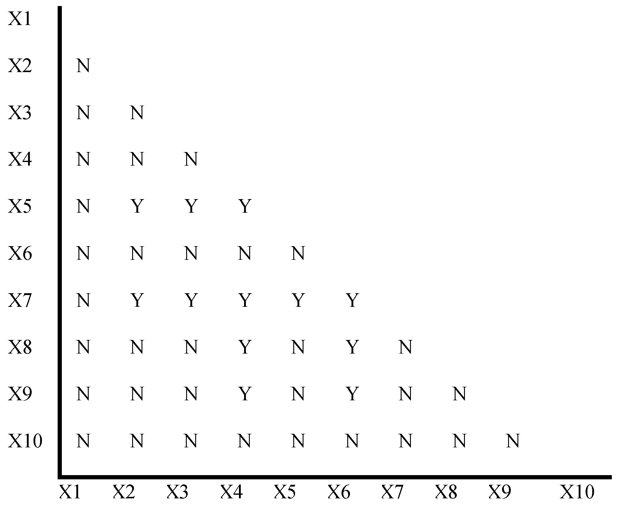
| Factors | Precipitation (X1) | Temperature (X2) | Residential Area Distance (X3) | Road Distance (X4) | Population (X5) | Water Distance (X6) | Soil (X7) | Altitude (X8) | Slope (X9) | Aspect (X10) |
|---|---|---|---|---|---|---|---|---|---|---|
| q value | 0.272 | 0.149 | 0.113 | 0.059 | 0.212 | 0.003 | 0.237 | 0.096 | 0.102 | 0.006 |
| p value | 0.000 | 0.000 | 0.000 | 0.000 | 0.000 | 0.000 | 0.000 | 0.000 | 0.000 | 0.000 |
Disclaimer/Publisher’s Note: The statements, opinions and data contained in all publications are solely those of the individual author(s) and contributor(s) and not of MDPI and/or the editor(s). MDPI and/or the editor(s) disclaim responsibility for any injury to people or property resulting from any ideas, methods, instructions or products referred to in the content. |
© 2024 by the authors. Licensee MDPI, Basel, Switzerland. This article is an open access article distributed under the terms and conditions of the Creative Commons Attribution (CC BY) license (https://creativecommons.org/licenses/by/4.0/).
Share and Cite
Xia, X.; Liang, W.; Lv, S.; Pan, Y.; Chen, Q. Remote Sensing Identification and Stability Change of Alpine Grasslands in Guoluo Tibetan Autonomous Prefecture, China. Sustainability 2024, 16, 5041. https://doi.org/10.3390/su16125041
Xia X, Liang W, Lv S, Pan Y, Chen Q. Remote Sensing Identification and Stability Change of Alpine Grasslands in Guoluo Tibetan Autonomous Prefecture, China. Sustainability. 2024; 16(12):5041. https://doi.org/10.3390/su16125041
Chicago/Turabian StyleXia, Xingsheng, Wei Liang, Shenghui Lv, Yaozhong Pan, and Qiong Chen. 2024. "Remote Sensing Identification and Stability Change of Alpine Grasslands in Guoluo Tibetan Autonomous Prefecture, China" Sustainability 16, no. 12: 5041. https://doi.org/10.3390/su16125041