Abstract
Landslides are common natural disasters that cause serious damage to ecosystems and human societies. To effectively prevent and mitigate these disasters, an accurate assessment of landslide hazards is necessary. However, most traditional landslide hazard assessment methods rely on static assessment factors while ignoring the dynamic changes in landslides, which may lead to false-positive errors in the assessment results. This paper presents a novel landslide hazard assessment method for the Zagunao River basin, China. In this study, an updated landslide inventory was obtained for the Zagunao River basin using data from interferometric synthetic aperture radar (InSAR) and optical images. Based on this inventory, a landslide susceptibility map was developed using a random forest algorithm. Finally, an evaluation matrix was created by combining the results of deformation rates from both ascending and descending data to establish a hazard level that considers surface deformation. The method presented in this study can reflect recent landslide hazards in the region and produce dynamic assessments of regional landslide hazards. It provides a basis for the government to identify and manage high-risk areas.
1. Introduction
Landslides is defined as the downward movement of soil or rock due to gravity and natural factors like rainfall, earthquakes, and human activities such as excavation [1,2,3]. They occur more frequently in urbanized slopes [4,5,6], earthquake-prone regions [7], and areas with heavy rainfall [8,9]. These geological hazards pose a significant threat, causing substantial damage to both natural and human environments [10]. From 2000 to 2017, landslides led to an estimated economic loss of around USD 50 billion and over 32,000 fatalities worldwide [11]. Therefore, conducting hazard assessments to identify at-risk areas and implementing preventive measures are crucial for effective risk mitigation.
Landslide hazard assessment is the process of analyzing and evaluating the likelihood of landslides and their possible consequences. It is an important component of landslide investigations and landslide risk management [12,13]. The process typically includes three main steps: (1) creating a landslide inventory, (2) creating a landslide susceptibility map, and (3) performing a landslide hazard assessment [14,15]. The landslide inventory is the basis for a landslide hazard assessment, and its accuracy and completeness directly affect the reliability of the assessment [16,17]. Various technologies and methods may be used to create a landslide inventory, including drone photogrammetry, high-resolution satellite optical imagery, laser scanning interpretation, and field surveys [18,19]. Landslide susceptibility reflects the probability of a landslide occurring [5,20,21]. Landslide hazard assessments, based on susceptibility results, consider triggering factors such as rainfall or earthquakes [12].
Traditional regional hazard assessments can provide essential guidance for government planning and land management but often focus on static disaster risk situations. Previous studies on regional landslide disasters have often been based on landslide inventories and statistical analyzes of the correlation between landslides and causal factors to achieve regional disaster assessments and classifications [22,23,24,25]. Some researchers have employed specialized software for safety factor analysis on typical slopes with stability hazards to quantitatively assess landslide hazards. However, this method is limited to specific areas and shallow-to-moderate-depth landslides, making it less widely applicable [26]. Physics-based models have been developed to assess climate-induced landslides, adaptable to various types, and suitable for medium- or larger-scale assessments. Yet, these models lack long-term updates and cannot evaluate landslide disasters within specific periods [27]. Geological-climatic models, using annual precipitation’s characteristic values and terrain indices, estimate landslide occurrence frequencies, assessing landslide disaster risks with significant uncertainties [28]. With the increase in economic development and human activities, as well as the dilution of risk awareness and overreliance on different protective measures [29,30,31], areas with a moderate to high landslide risk are widespread. This leads to challenges for governments in effectively using and developing resources, as well as in categorizing previously controlled high-risk areas as moderate to high risk in landslide assessments. Therefore, traditional disaster assessment methods are inadequate to meet the current global demands for landslide risk management and prevention.
Synthetic aperture radar (SAR) imaging is an active microwave remote sensing technology, which is widely used on several platforms [32]. The active imaging mode and insensitivity to weather make it possible to obtain the ground surface SAR image periodically, thereby enabling it to detect the surface movement caused by the geological hazard (e.g., landslides, surface subsidence, and earthquakes) with multiple SAR images [33]. The time-series interferometric synthetic aperture radar (InSAR) technology was developed based on multiperiod SAR images to extract surface deformation with a millimeter-level accuracy [34]. Therefore, incorporating the deformation data obtained through InSAR into landslide hazard assessments addresses the current requirements for dynamic landslide hazard management.
The advancement of InSAR technology has facilitated the evaluation of hazards associated with recent landslides. Various InSAR methods have been extensively used in the assessment of landslide hazards, including multitemporal InSAR (MT-InSAR) [35], persistent scatterer InSAR (PSInSAR) [34,36], small baseline subset InSAR (SBAS-InSAR) [37,38,39], and DInSAR [40]. However, the Zagunao River basin frequently experiences landslides, and there is a lack of hazard level maps. Currently, the application of InSAR in the Zagunao River basin has primarily focused on identifying landslide locations and triggering factors. To better assess the landslide hazards in the Zagunao River basin, this study proposes a novel method for assessing landslide hazards by combining deformation results from ascending and descending SAR data images. First, integrated remote sensing technologies are adopted to generate the latest landslide inventory for the Zagunao River basin. Then, susceptibility assessments are conducted using the random forest (RF) method. Finally, the method categorizes and combines the InSAR deformation results obtained from different orbits of SAR images to propose a landslide hazard assessment matrix and create a landslide hazard map for the study area.
2. Study Area
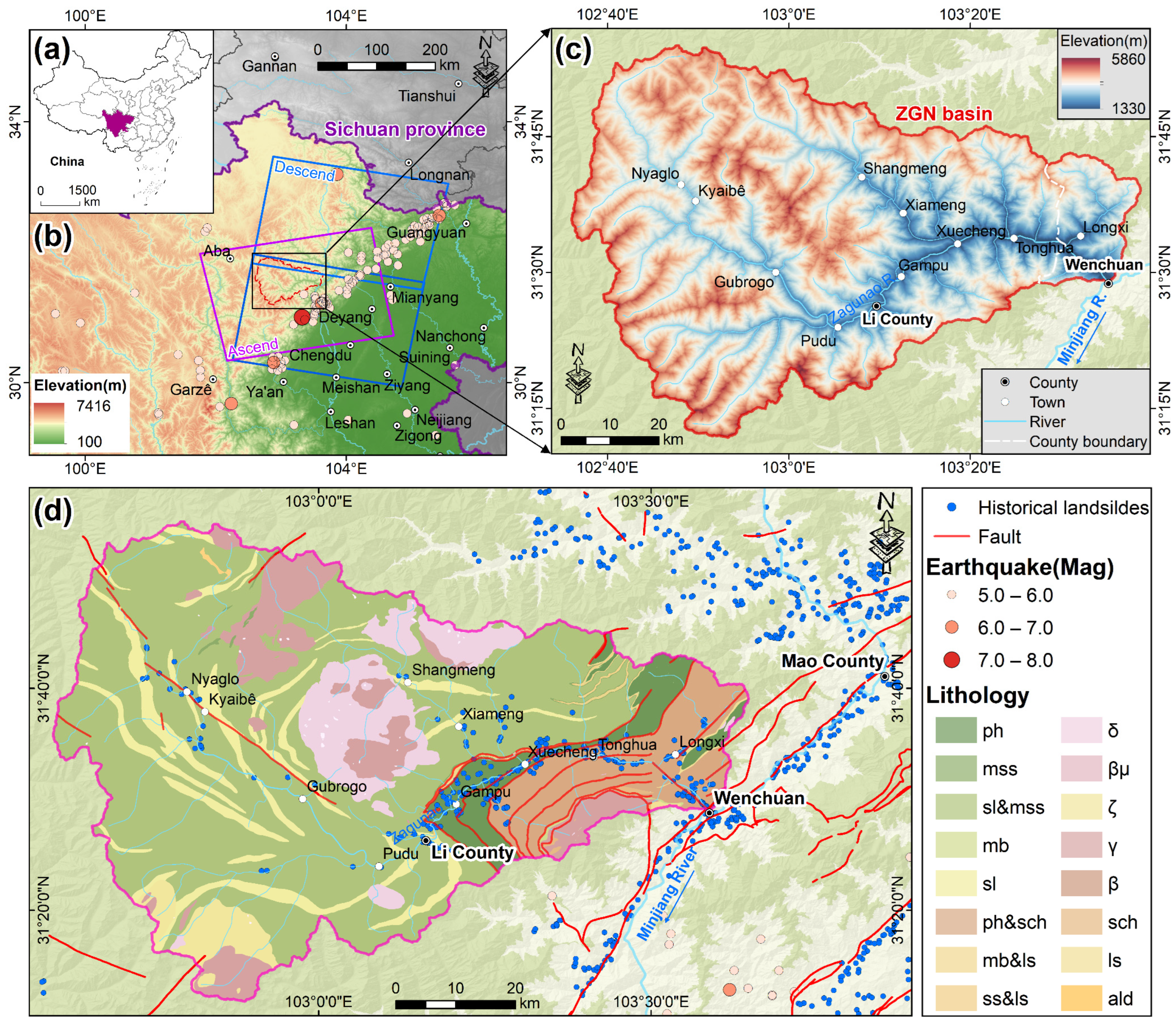
The Zagunao River is an upper tributary of the Minjiang River, located in the central part of Sichuan Province, China (Figure 1a). It was one of the areas that was severely affected during the 2008 Wenchuan earthquake. The main branch of the Zagunao River is approximately 168 km long, and it has major tributaries such as the Mengdong River and Laisu River. The total drainage area of the basin is approximately 4629 km2, which spans from 102°36′E to 103°38′E and from 31°11′N to 31°54′N (Figure 1b). The highest elevation in the basin is 5860 m and the lowest elevation is 1330 m, with a relative altitude difference of up to 4530 m, which is typical of an alpine and gorge region (Figure 1c). The region has a subtropical monsoon climate, with annual rainfall ranging from 650 to 1000 mm, with more than 70% concentrated in the summer, and average annual temperatures range from 6.9 to 11 °C [41]. Figure 1d displays the geological overview and historical landslide distribution in the Zagunao River basin, with the data provided by the Resource and Environmental Science and Data Center (http://www.resdc.cn (accessed on 17 February 2023)). Historically, due to the frequency of earthquakes in the region and increasing human activities related to social and economic development, numerous ancient landslides have occurred, resulting in catastrophic human and property loss. These conditions have also contributed to the occurrence of new landslides in the area.
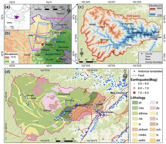
Figure 1.
Location and overview of the study area: (a) location of Sichuan Province; (b) coverage area of Sentinel-1 satellite imagery in the study area and distribution of historical earthquakes; (c) topography and geomorphology of the study area; (d) geological strata, faults, and distribution of historical landslides in the study area.
3. Data and Methodology
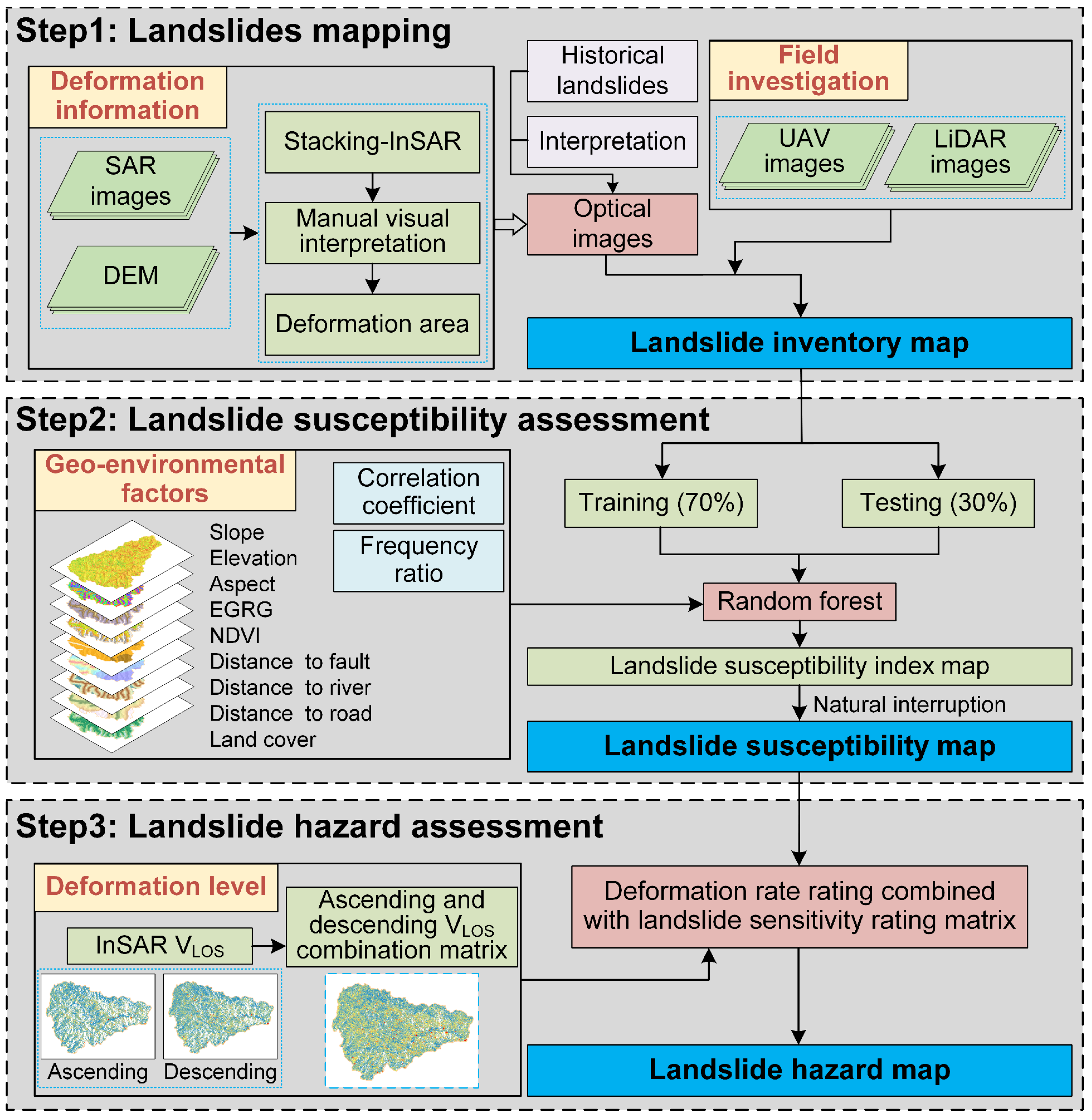
The technical workflow of this study includes three main steps (Figure 2). Firstly, InSAR deformation information is used to identify the potential areas of landslides. Optical imagery is also used to refine the boundaries of landslides, which results in spatial distribution data for active landslides. Historical landslide databases and optical imagery are employed to identify ancient landslide features within the study area. Field surveys (including UAV and airborne LiDAR technology) are conducted to validate the landslide inventory for the study area. Secondly, based on the landslide inventory map in Step 1, landslide susceptibility is assessed using a random forest model and the natural breaks method. Finally, InSAR technology is employed to obtain surface deformation by combining ascending and descending orbit data. This deformation information is then integrated with the landslide susceptibility map to generate landslide hazard levels that account for the deformation factors within the study area.
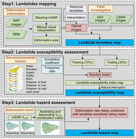
Figure 2.
Technical workflow of the study.
3.1. Dataset
Creating a landslide inventory forms the foundation of landslide susceptibility assessments [42]. Various methods and technologies can be employed to generate reliable and precise landslide inventories. For instance, integrated remote sensing techniques and new data have been used in numerous studies, with their advantages and limits discussed [43]. Consequently, this study employed three methods to collect landslide data, including the interpretation of optical imagery from Google Earth (70 landslides were identified), field surveys combined with stacking-InSAR technology (49 landslides were identified), and historical landslide records (9 landslides were identified). In the end, within the study area, 128 landslides were identified, with 70% (90 landslides) used for model construction and the remaining 30% (38 landslides) used for model validation.
This study collected Sentinel-1A SAR image data of the Zagunao River basin provided by ESA. The data included ascending data from 11 January 2020 to 24 January 2022 (117 scenes), and descending data from 4 January 2019 to 2 December 2022 (114 scenes). The coverage area and specific parameter information for these data are illustrated in Figure 1b and Table 1.

Table 1.
Basic parameters of Sentinel-1 radar satellite image used in the study.
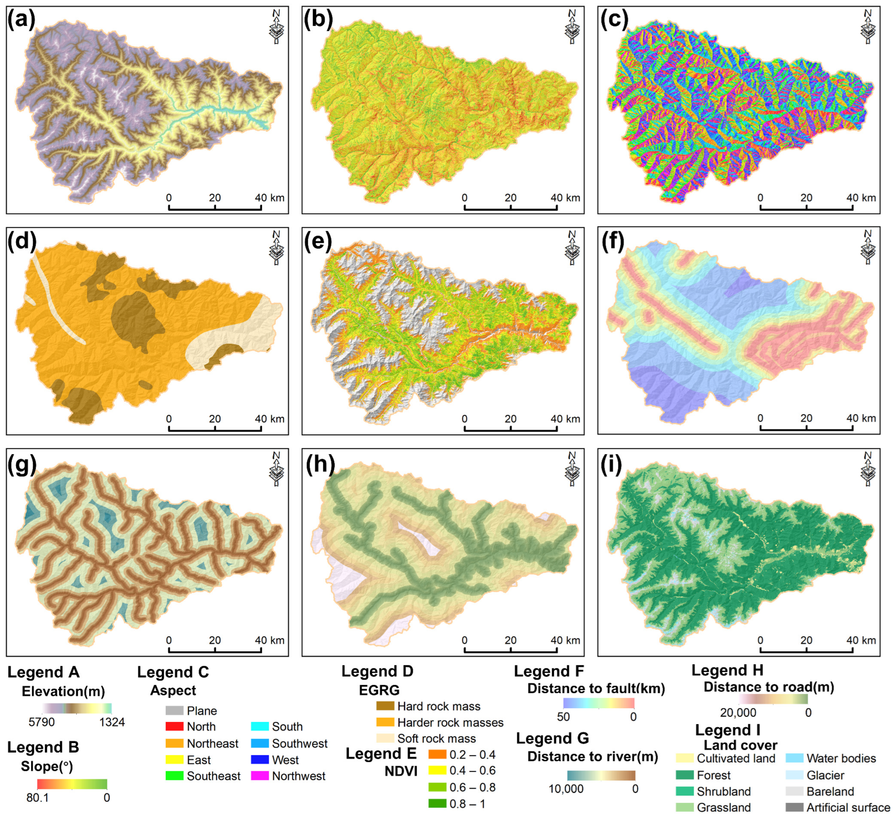
Landslides result from the combined effects of influencing factors [44]. Selecting appropriate influencing factors is crucial for building landslide assessment models, but there is currently no standardized method [45]. In this study, the influencing factors for landslides were determined based on the characteristics of the geological environment, a previous literature analysis, and data availability [46]. We selected nine landslide condition factors to predict the spatial susceptibility of landslides: slope, aspect, elevation, distance to roads, distance to rivers, distance to faults, normalized difference vegetation index (NDVI), engineering geological rock group, and land use. A digital elevation model (DEM) with a 30 m resolution served as the basis for the thematic maps, and the terrain factors were extracted from ASTER GDEM data. These datasets are available from the National Aeronautics and Space Administration (NASA) website (https://www.earthdata.nasa.gov/ (accessed on 25 February 2023)). Using ArcGIS software (version: 10.8), three terrain factor maps were generated from the DEM data (Figure 3a–c). Buffer analysis maps for rivers, roads, and fault lines were created in ArcGIS software (Figure 3f–h).
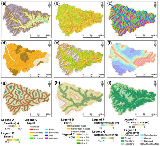
Figure 3.
Landslide influencing factors: (a) elevation; (b) slope; (c) aspect; (d) engineering geological rock group; (e) NDVI; (f) distance to faults; (g) distance to rivers; (h) distance to roads; (i) land cover.
The slope and aspect factors are both derived from the DEM. The slope is a critical factor in landslide occurrences. Within a certain threshold, steeper slopes are associated with a higher likelihood of landslides. The aspect indicates the direction of the slope and is typically categorized into nine classes, including flat, north, northeast, east, southeast, south, southwest, west, and northwest.
Geological materials, including rocks and soils, form the material foundation for landslide development [47]. They have a direct effect on the stability of slopes and the ease of surface erosion [48]. Different geological materials possess varying levels of inherent strength and resistance to weathering. In this study, the geological strata in the study area were classified into three categories based on the type of geological material, physical-mechanical properties, and structural characteristics:
Weak rocks: these rocks have a lower inherent strength and are less resistant to weathering. Moderately hard rocks: these rocks exhibit an intermediate strength and weathering resistance. Hard rocks: this category includes rocks with a high inherent strength and strong resistance to weathering.
Vegetation coverage is a crucial factor influencing slope stability. Therefore, this study used the NDVI as an indicator for the vegetation coverage analysis and mapping. The NDVI reflects the growth status of vegetation and changes in soil structure [49]. In this research, the NDVI was calculated using Sentinel-2A multispectral imagery, and the calculation formula can be found in reference [50].
Road and river data were sourced from the 1:250,000 National Basic Geographic Database (National Geographic Information Resource Catalogue Service System, https://www.webmap.cn/ (accessed on 9 December 2023)), while fault data were obtained from the National 1:200,000 Digital Geological Map Spatial Database. A buffer analysis of these datasets was conducted using ArcGIS 10.8 as part of this study.
Land use is an indirect factor that affects landslide occurrences primarily by altering certain factors such as soil erosion, rainfall infiltration, and surface structure, which subsequently impact slope stability [51]. In this study, GlobeLand30: Global Geospatial Information Public Product (http://www.globallandcover.com/ (accessed on 17 April 2023)) was used as the data source for land use. It was categorized into nine types, including cropland, forestland, shrubland, grassland, bare land, water bodies, glaciers, and artificial surfaces.
3.2. Susceptibility Assessment
3.2.1. Frequency Ratio
The frequency ratio (FR) model is an effective geospatial tool for estimating the likelihood of landslides occurring in a certain area within a specific period [52]. Based on the assumptions of landslide susceptibility analyses, future landslides are expected to occur under similar conditions to historical landslides [53]. The formula for calculating the FR is as follows:
where N represents the landslide area corresponding to each factor, is the total area of the landslides, S represents the area of each specific factor level, and is the total area of the study area.
3.2.2. Random Forest
The RF model is a machine learning method that uses multiple decision trees for classification or regression and can provide approximate results that are similar to Bayesian classifiers [54]. Unlike other models, the RF model can provide various measures of variable importance, with the most reliable measure being the reduction in classification accuracy when the values of variables in the trees are randomly permuted [55]. When solving classification problems, random forest predictions are considered unweighted majority class votes [56]. The bagging technique is used to select training datasets for model calibration from random samples of variables. For each variable, this function determines the model’s prediction error if the values of that variable are permuted in out-of-bag observations [57,58].
In landslide susceptibility mapping, the random forest model leverages the diversity among trees, allowing each tree to vote for categories, and the final category is determined based on the majority vote [59]. This ensemble method demonstrates robust and accurate performance on complex datasets, requires minimal parameter tuning, and exhibits a tolerance to many noisy variables [60].
3.3. Landslide Hazard Assessment
3.3.1. The Division of Deformation Levels
Using SBAS-InSAR technology, surface deformation rates can be obtained and used to analyze the historical deformation characteristics of landslides. Due to the varying susceptibility of different satellite orbits to deformation in different directions, deformation information from a single orbit can be incomplete, which leads to variations in the deformation results from different orbits. To address this situation, a matrix was constructed in this study to merge the deformation rates obtained from the ascending and descending data (Table 2). Zhou et al. (2022) [35] used intervals of 2 mm/month to classify deformation rate maps into four levels. Considering the conditions of the study area, the natural breaks method was used in this study to classify the deformation rates. For the ascending orbit data, the classification was as follows: V1 (0–0.40 mm/month), V2 (0.40–0.94 mm/month), V3 (0.94–1.70 mm/month), V4 (1.70–3.31 mm/month), and V5 (>3.31 mm/month). For the descending orbit data, the classification was as follows: V1 (0–0.40 mm/month), V2 (0.40–0.91 mm/month), V3 (0.91–1.73 mm/month), V4 (1.73–3.50 mm/month), and V5 (>3.50 mm/month).
Table 2.
Combination matrix of surface deformation rate levels for ascending and descending orbit data.
3.3.2. Landslide Hazard Zonation
Landslides are dynamic processes, and their hazard levels fluctuate over time. Time-series InSAR technology allows for the monitoring of the slope deformations in the study area over a temporal sequence. Incorporating InSAR deformation rates as a time probability factor into landslide hazard assessments effectively reduces the interference of temporal changes on the assessment results. Currently, regional landslide hazard assessments are primarily based on historically recorded landslide data, which neglect the dynamic changes in landslides. This approach can lead to outdated and inaccurate results in regional landslide hazard assessments. Time-series InSAR technology can reveal the temporal patterns of landslides. By combining the deformation information obtained through InSAR technology with landslide susceptibility assessments, landslide hazards can be dynamically evaluated. The matrix method, as referenced in Dai et al. (2022) [38], combines the deformation rate levels (including ascending and descending orbit data) with landslide susceptibility to provide a joint assessment. The evaluation matrix is shown in Table 3.
Table 3.
Combination of deformation rate levels and landslide susceptibility assessment levels.
4. Results
4.1. Landslide Inventory Map
Based on the stacking-InSAR technique, using Sentinel-1A ascending and descending orbit data from 2019 to 2022 and in conjunction with Google Earth imagery, the deformation targets were extracted. Field investigations and drone photography were conducted for a ground-truth validation of the visual interpretation results, and corrections were made to the landslide boundaries. The obtained landslides are shown in Figure 4 and Figure 5.

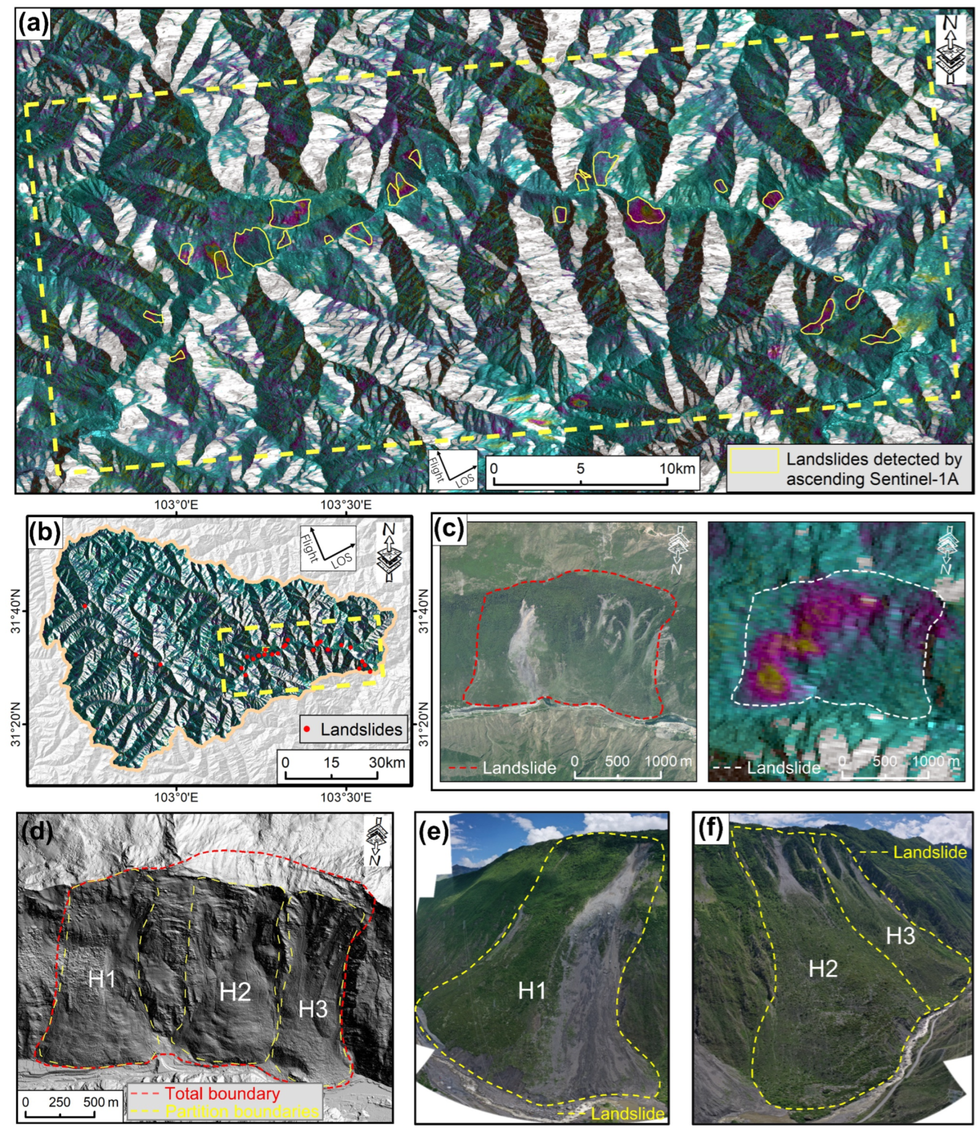
Figure 4.
Landslide detection results of stacking-InSAR based on ascending orbit data using: (a) InSAR phase results in the landslide concentration area; (b) InSAR phase results in the study area; (c) typical landslides; (d) hillshade generated from LiDAR point cloud data; (e) drone imagery of Landslide H1; (f) drone imagery of Landslides H2 and H3.
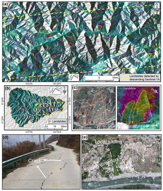
Figure 5.
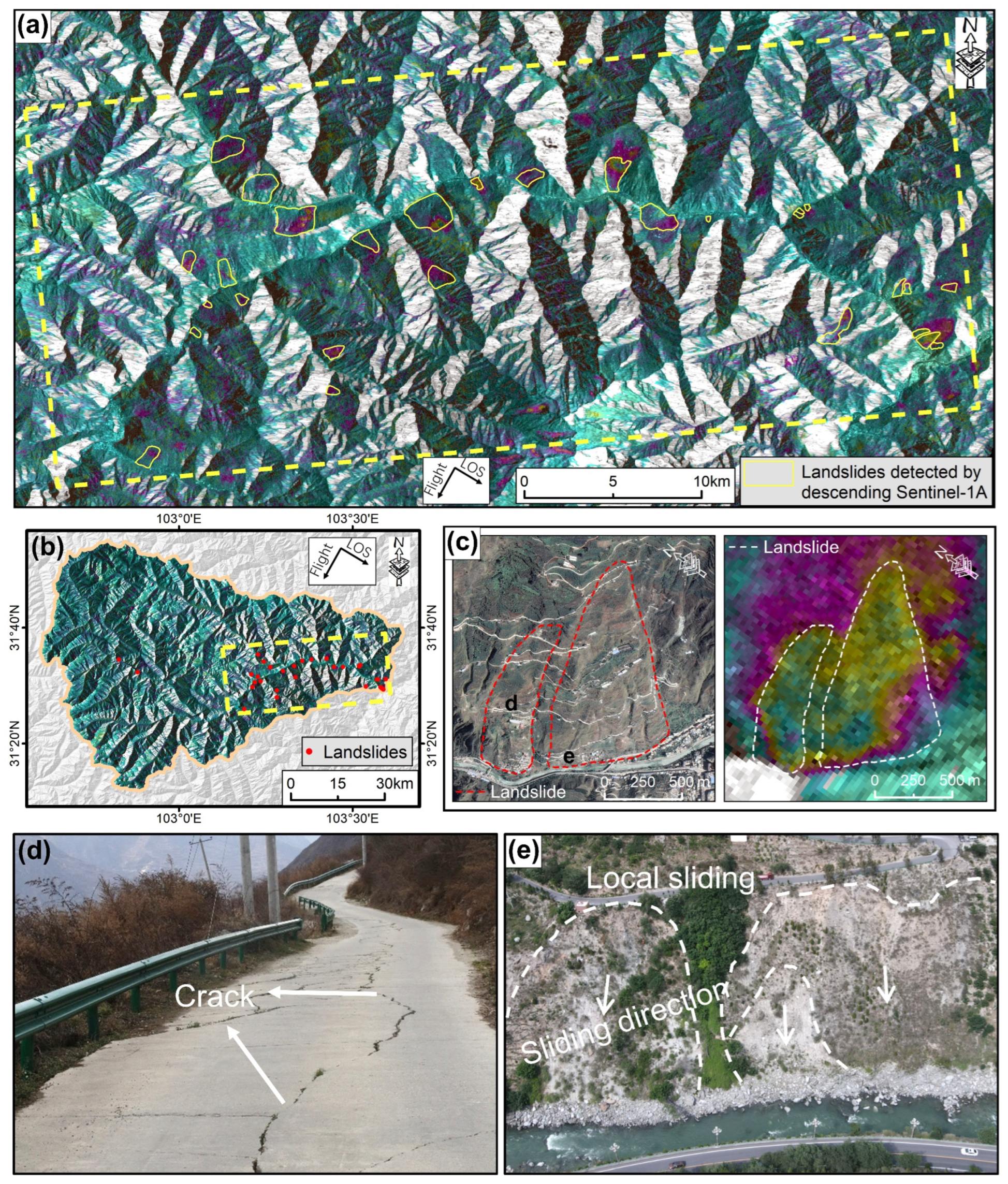
Landslide detection results of stacking-InSAR based on descending orbit data: (a) InSAR phase results in the landslide concentration area; (b) InSAR phase results in the study area; (c) optical images of typical landslides along with their boundary extents and overlaid InSAR results; (d) distribution of cracks in the middle of a landslide; (e) collapse at the frontal area of a landslide.
Figure 4 displays the landslide monitoring results obtained based on the ascending orbit data. A total of 26 landslides were detected, which were located mainly on both sides of the Zagunao River in the eastern part of the study area. The distribution map of the landslides can be seen in Figure 4a,b. Figure 4c shows typical landslide optical imagery, boundary extents, and InSAR results. We conducted a more detailed investigation of the landslide group using airborne LiDAR data (Figure 4d) and drone optical imagery (Figure 4e,f) and divided them into three landslides: H1, H2, and H3. The hillshade generated from airborne LiDAR data and drone optical imagery revealed clear signs of deformation and accumulation.
The results of the landslide detection based on the descending orbit data are shown in Figure 5. A total of 31 landslides were detected, 8 of which were also detected in the ascending orbit data. The distribution of these landslides is illustrated in Figure 5a,b, which is similar to the landslide distribution detected in the ascending orbit data. Figure 5c displays optical images of two typical landslides with very distinct deformation patterns, showing their boundary extents and overlaid InSAR results. Field verification revealed extensive residential areas in the frontal regions of these two landslides, with numerous cracks appearing in roads and walls (Figure 5d). There were also clear signs of collapse and deformation in the frontal areas of the landslides (Figure 5e).
Concerning the historical landslide database and using optical imagery, 79 additional landslides were identified and added, which updated the landslide inventory in the Zagunao River basin. In total, there were 128 landslides in the study area, covering an approximate area of 44 km2. Among these, 49 landslides were detected through InSAR interpretation (26 from ascending orbit data, 31 from descending orbit data, and 8 detected by both), while the remaining 79 landslides were identified through optical interpretation.
4.2. Landslide Susceptibility Map
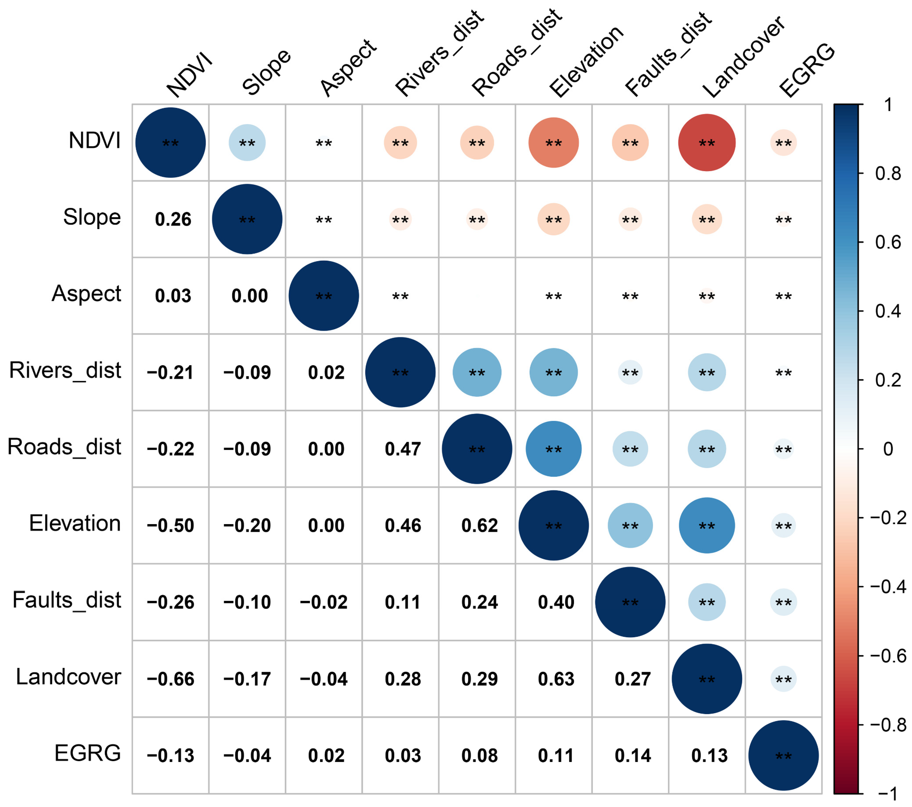
In a landslide susceptibility assessment, the choice of evaluation factors is a crucial step. More factors do not always result in better outcomes; instead, a balance between quantity and quality is essential. The selected factors should not only reflect the impact of the factors on landslides but also avoid strong correlations among them. In this study, nine influencing factors, including elevation, slope, slope aspect, engineering geological lithology, NDVI, distance to rivers, distance to faults, distance to roads, and land cover, were chosen as indicators for modelling the landslide susceptibility in the study area. A Pearson correlation coefficient analysis was used to assess the correlations among these evaluation factors. The Pearson correlation coefficient is a method for measuring the linear relationship between multiple continuous variables, denoted by “r” with values ranging from −1 to 1. The sign indicates the direction of the correlation, and the absolute value represents the strength. Generally, |r| < 0.3 suggests no correlation, |r| < 0.5 indicates a weak correlation, and |r| > 0.8 indicates a strong correlation [61]. Figure 6 displays the correlation coefficients among the factors. All the coefficients among the factors were less than 0.8; and most of them were less than 0.5. This suggests that the ten selected factors did not exhibit strong correlations with each other and were suitable for landslide susceptibility modelling.
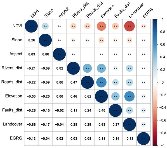
Figure 6.
Pearson’s correlations among landslide conditioning factors. (Roads_dist represents the distance to roads; EGRG represents engineering geological lithology; Faults_dist represents the distance to faults; Rivers_dist represents the distance to rivers; ** is a significance marker).
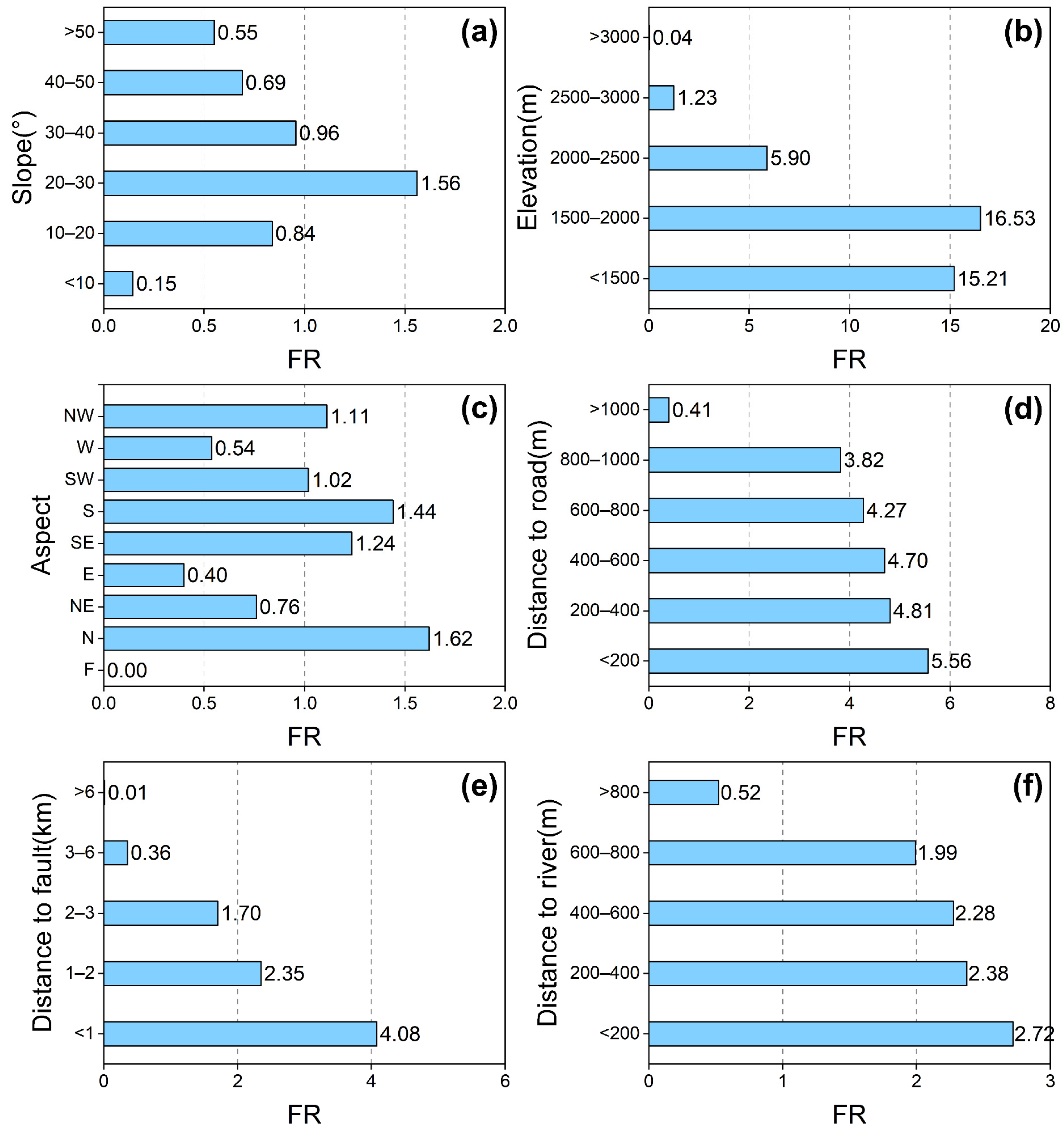
By calculating the FR values of various influencing factors, we can identify the spatial relationships among landslide occurrences and regulating factors. The slope angle is related to the variation in slope shear stress, and an increase in slope angle within a certain range may lead to landslide occurrences [62]. The FR analysis indicated that the highest probability of landslides fell within the 20–30° range, reaching 1.56, which was consistent with the previous analysis. The FR values for the other categories decreased in the following order: 30–40° (0.96), 10–20° (0.84), 40–50° (0.69), >50° (0.55), and <10° (0.15) (Figure 7a). Regarding elevation, the analysis indicated that the highest number of landslide pixels detected, and the highest FR value (16.53) were found in the elevation range of 1500–2000 m (Figure 7b). In terms of aspect, the highest FR value was found for north-facing slopes (1.62). In the remaining eight directions, slopes facing south, southeast, northeast, northwest, southwest, and east–northeast also had relatively high probabilities of landslide occurrence (with FR values of 1.44, 1.24, 1.11, 1.02, and 0.76, respectively). In contrast, slopes facing east or west and flat slopes had lower FR values, with values of 0.4, 0.54, and 0, respectively (Figure 7c). Regarding the distance to roads, faults, and rivers, higher landslide occurrence probabilities were associated with closer proximities. Specifically, FR values were highest (5.56) within <200 m from the road (Figure 7d), highest (4.08) within the area <1 km from the fault (Figure 7e), highest (5.56) within the area <200 m from the river (Figure 7f) and decreased gradually with the increasing distance. Analyzing the association between landslides and engineering geological lithology (EGRG) revealed that landslides were most likely to occur in soft rock, followed by relatively hard rock and hard rock lithology (Figure 7i). The FR analysis of the NDVI showed that lower NDVI values indicated higher landslide susceptibility. The FR values for NDVI groups 0.2–0.4, 0–0.2, 0.4–0.6, 0.6–0.8, and 0.8–1 were 2.84, 0.57, 0.52, 0.38, and 0.07, respectively (Figure 7h). Additionally, the effects of eight land cover types on landslide occurrence were assessed. The results showed that agricultural areas had the highest FR value, indicating the highest probability of landslides in the area. Other landslides were mainly distributed in shrubland, woodland, and grassland areas (Figure 7g).
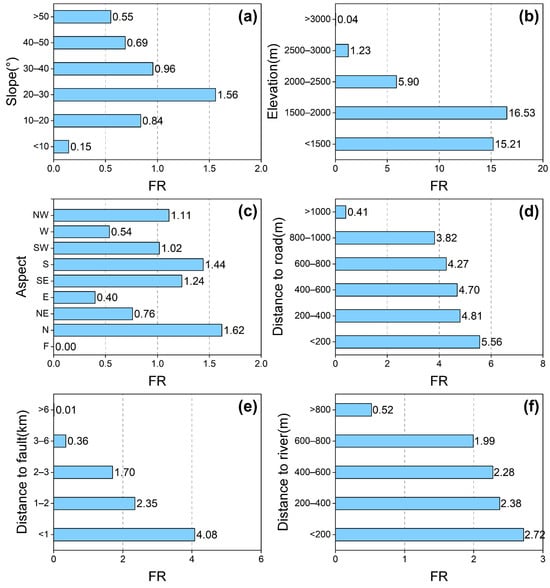
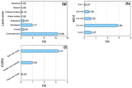
Figure 7.
Relationship between landslides and the conditioning factors: (a) slope; (b) elevation; (c) aspect; (d) distance to roads; (e) distance to faults; (f) distance to rivers; (g) land use; (h) NDVI; (i) engineering geology rock group.
Following landslide factor correlation and FR analyses, the next step is to create a landslide susceptibility map, which is an effective tool for predicting the occurrence of landslides. In this study, a landslide susceptibility map was developed in four steps. The first step involved using ArcGIS software to create a grid within the study area and extract information on various landslide regulating factors. The second step involved establishing a model using a training dataset and then calculating the landslide susceptibility index (LSI) for each grid based on the trained trends. In the next step, all grid LSIs were transferred back to ArcGIS, and the landslide susceptibility map was created by visualizing the LSIs. Finally, the landslide susceptibility map was divided into five categories (Figure 8c) using the natural break method in ArcGIS: very low, low, moderate, high, and very high (Figure 8a). In this classification, high and very high susceptibility areas occupied 3.28% of the study area, which were primarily concentrated along both sides of the main stream of the Zagunao River. Moderate-susceptibility areas covered 3.71%, low-susceptibility areas covered 4.24%, and very low susceptibility areas covered 88.23% (Figure 8b). The receiver operating characteristic (ROC) curve (Figure 9) was used to assess the classification performance of the model [63]. The area under the curve (AUC) was 0.89, which is significantly higher than 0.5, indicating that the model had a high accuracy and discriminative power.
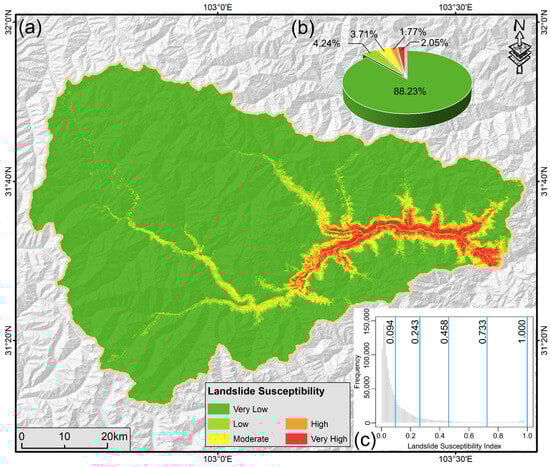
Figure 8.
Landslide susceptibility map: (a) spatial distribution of landslide susceptibility; (b) statistics of susceptibility areas in different categories; (c) classification using the natural breaks method.
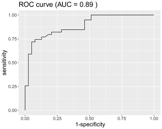
Figure 9.
ROC curve obtained for assessing model accuracy.
4.3. Landslide Hazard Map
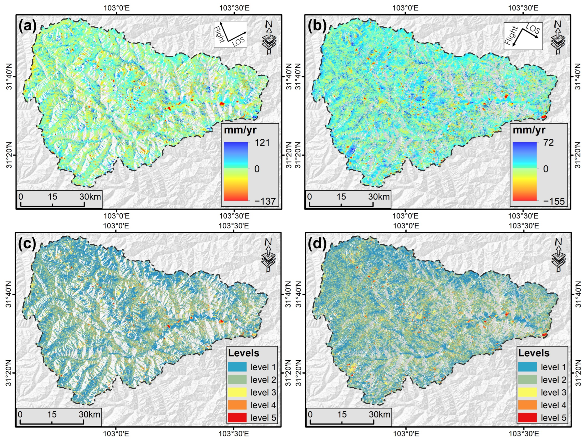
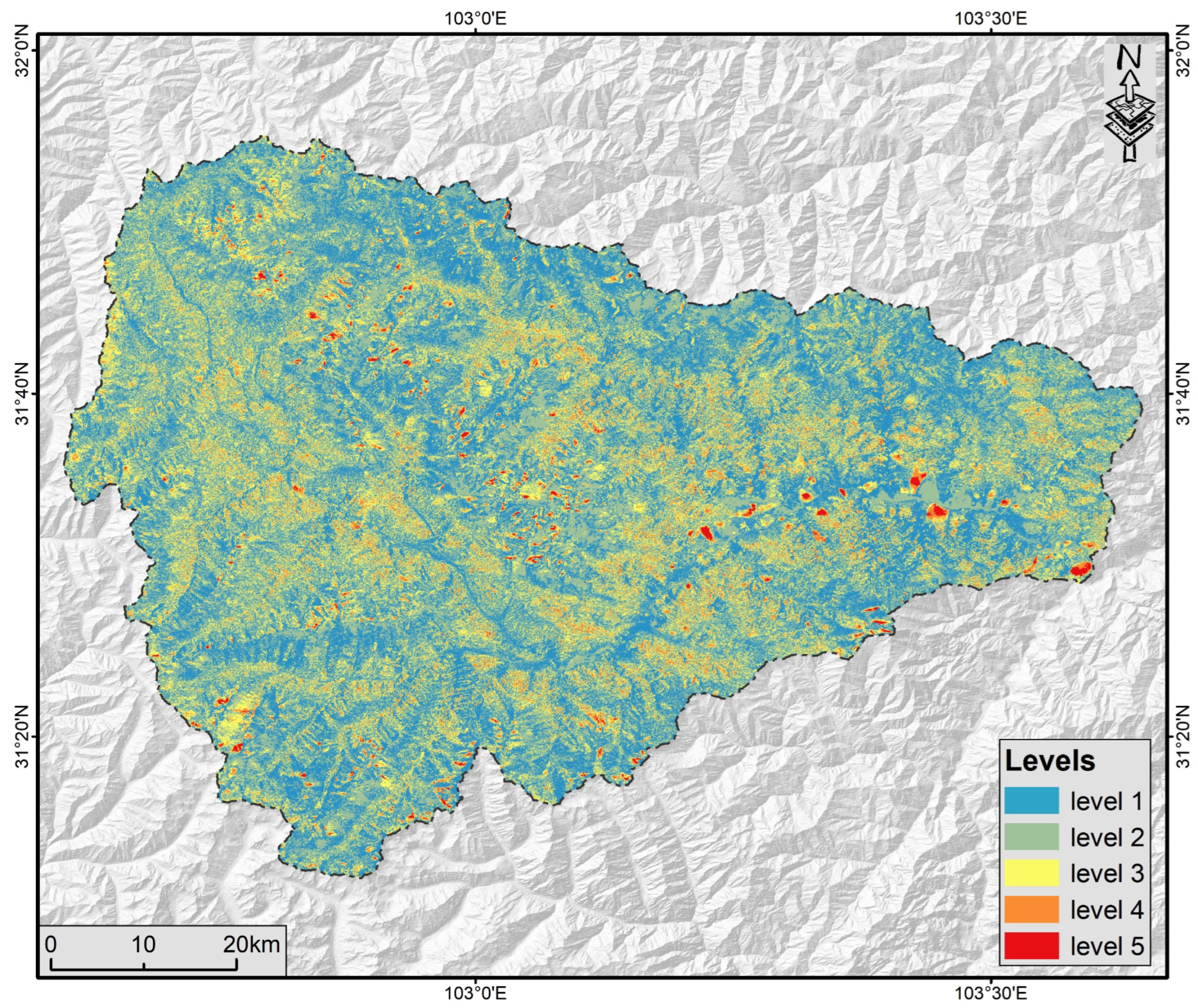
Deformation rates were obtained using the SBAS-InSAR method and reflected the deformation levels in the study area over the observation period. Blue points (negative values) indicate targets moving away from the satellite’s line of sight (LOS), red points (positive values) indicate targets moving closer to the satellite’s LOS, and green points represent relatively stable targets. The maximum annual deformation rates for the ascending data were −137 mm/year and 121 mm/year (Figure 10a). For the descending data, the maximum annual deformation rates were −155 mm/year and 72 mm/year, respectively (Figure 10b). The deformation rates of the ascending and descending data were classified into five classes according to the methodology described in Section 3.3.1 (Figure 10c,d). The deformation rates of the ascending and descending orbit data were merged according to the matrix in Table 2 and spatially interpolated using the ordinary kriging method to obtain the deformation rate map (Figure 11). The deformation rates were classified as very high (level 5), high (level 4), medium (level 3), low (level 2), and very low (level 1), with very high levels covering 0.48%, high levels covering 5.19%, medium levels covering 18.43%, low levels covering 38.43%, and very low levels covering 37.47%.
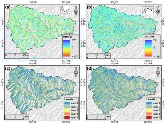
Figure 10.
Deformation rate maps and deformation rate classifications: (a) ascending-orbit deformation rate map; (b) descending-orbit deformation rate map; (c) classification of ascending-orbit deformation rates; (d) classification of descending-orbit deformation rates.

Figure 11.
Classification of ascending and descending orbits after the discriminant matrix.
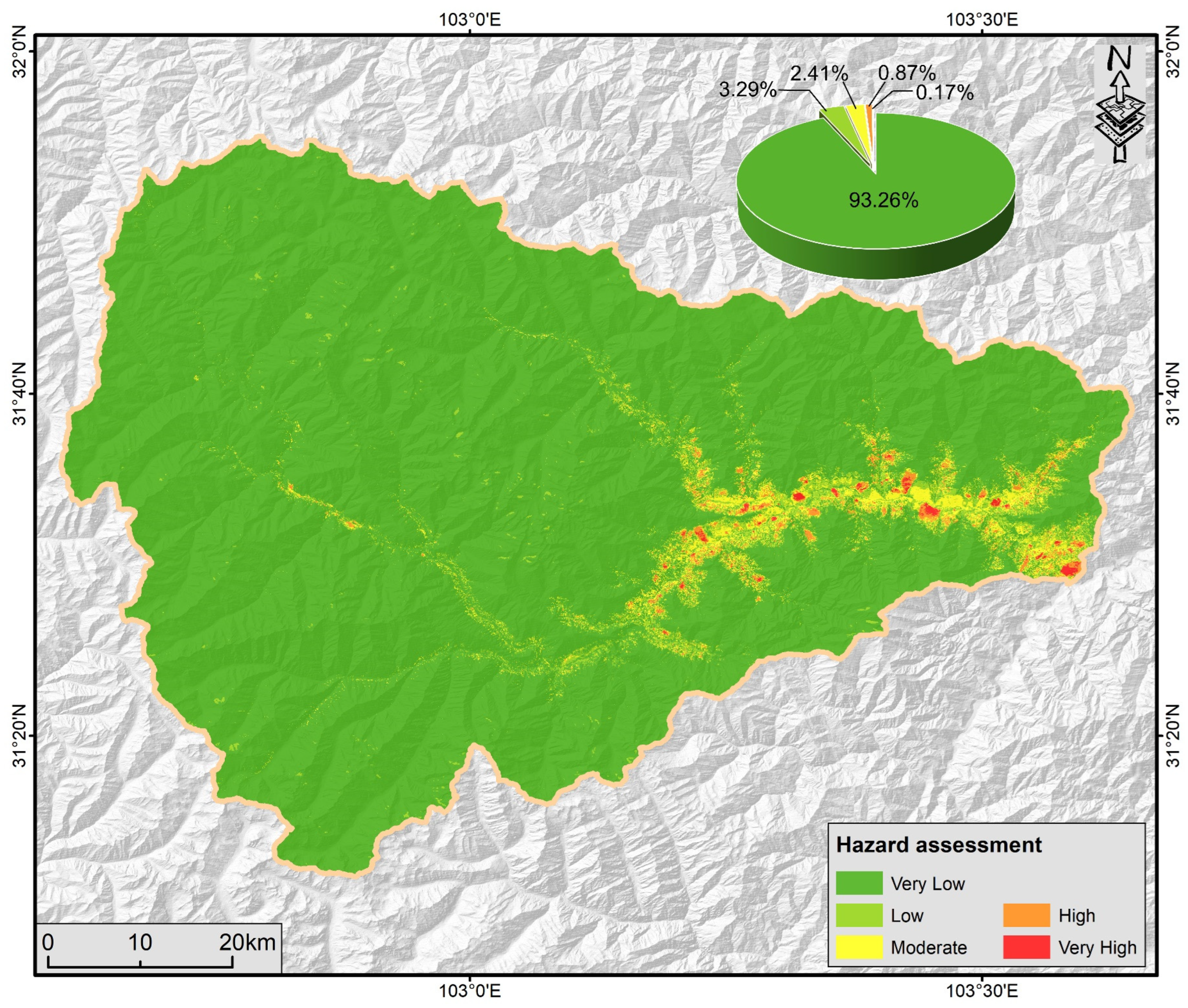
Based on the matrix in Table 3, combined with the landslide susceptibility results and surface deformation rates, the landslide hazard assessment level map for the Zagunao River basin was obtained (Figure 12): extremely high risk areas accounted for 0.17%, high-risk areas accounted for 0.87%, moderate-risk areas accounted for 2.41%, low-risk areas account for 3.29%, and very low risk areas accounted for 93.26% (Figure 12). The extremely high risk and high-risk areas were mainly distributed on both sides of the main Zagunao River. By providing the latest assessment results to relevant authorities, appropriate mitigation measures can be taken in high-risk areas, or the deformation rates of landslides can be directly controlled to reduce their level of risk. This evaluation method is conducive to saving resources, improving efficiency, and protecting human lives and property. Landslide evolution is a dynamic process, and the risk of landslides varies by geography. Time-series InSAR technology can efficiently monitor slope deformation rates, track slope deformation, and provide crucial data and possibilities for a dynamic landslide hazard assessment.
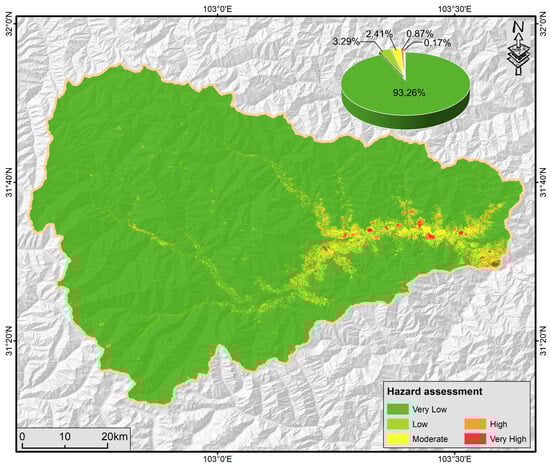
Figure 12.
Landslide hazard assessment results.
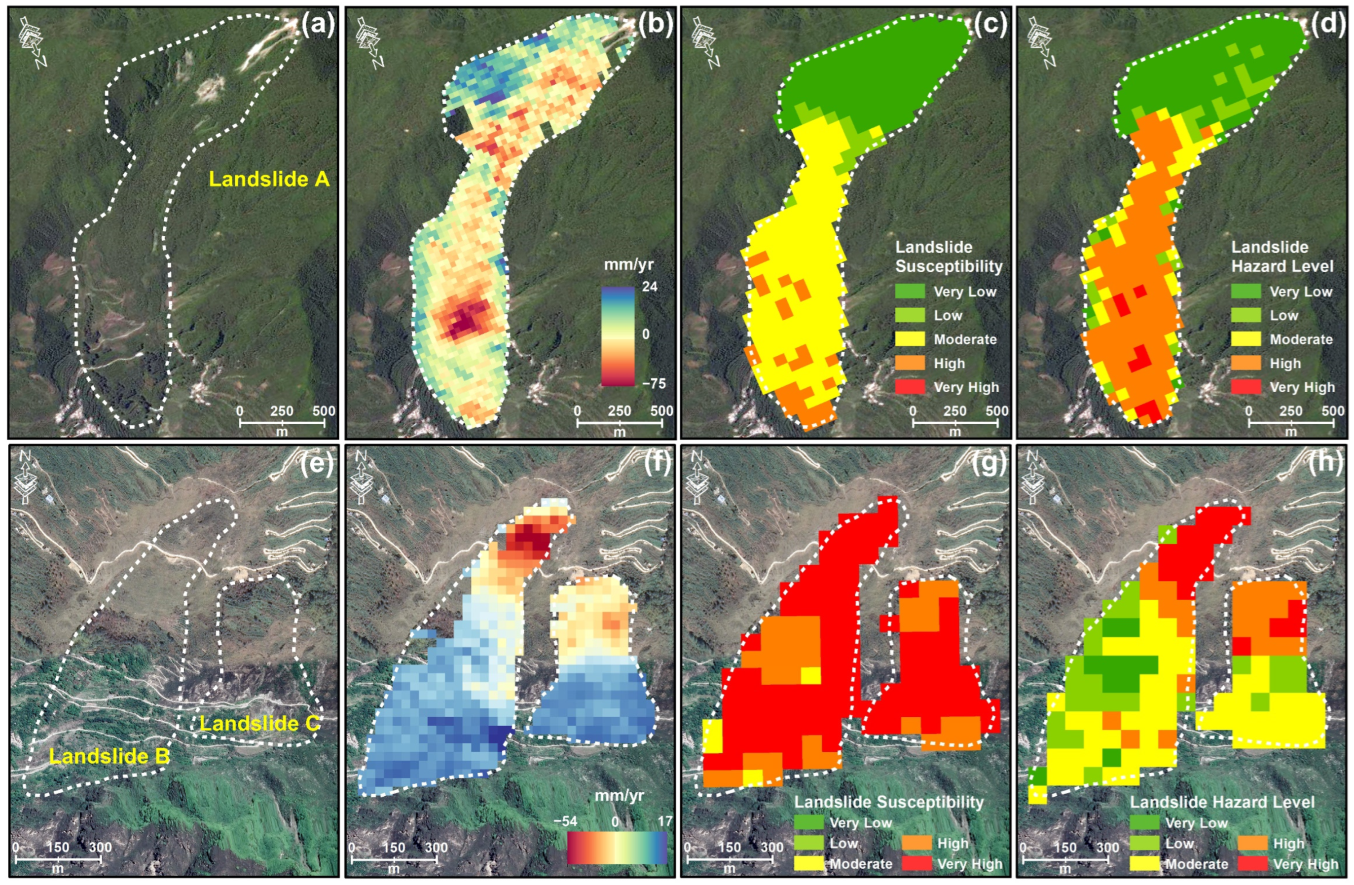
Susceptibility assessments focus on the spatial probability of landslides occurrence. However, when we incorporate time-series InSAR deformation data into a hazard assessment, temporal variability is considered. This integration significantly reduces the chances of false positives and false negatives in the assessment results and ultimately improves the accuracy of the results. To demonstrate this, we present three landslide cases: landslide A, landslide B, and landslide C (Figure 13a,e), all of which were located in the downstream section of the Zagunao River in Wenchuan County.

Figure 13.
Results of susceptibility and hazard assessment of a typical landslide: (a,e) optical images; (b,f) deformation rates; (c,g) results of susceptibility assessment; (d,h) results of hazard assessment.
The deformation area of landslide A was concentrated at the leading edge of the landslide (Figure 13b). In the susceptibility assessment, this region was classified as a moderately susceptible zone (Figure 13c), leading to an underestimated hazard level and resulting in false negatives. However, when we incorporated time-series deformation rates into the hazard assessment, this same area was categorized as a high-hazard zone (Figure 13d), providing a more realistic assessment.
In contrast, landslides B and C showed that deformation was concentrated towards the rear (Figure 13f). In the susceptibility assessment, the entire landslide was labelled as a highly susceptible area (Figure 13g), leading to a substantial overestimation of the hazard level and resulting in false positives. However, in the hazard assessment, the remaining areas were categorized as moderate-to-low-hazard zones (Figure 13h), improving the overall assessment results.
The integration of a spatiotemporal probability into hazard assessments effectively corrects the susceptibility results that rely on spatial probability. This integration offers more refined and accurate results, thereby providing essential guidance for government departments in their disaster prevention and mitigation efforts.
5. Discussion
5.1. SAR Geometry Effect
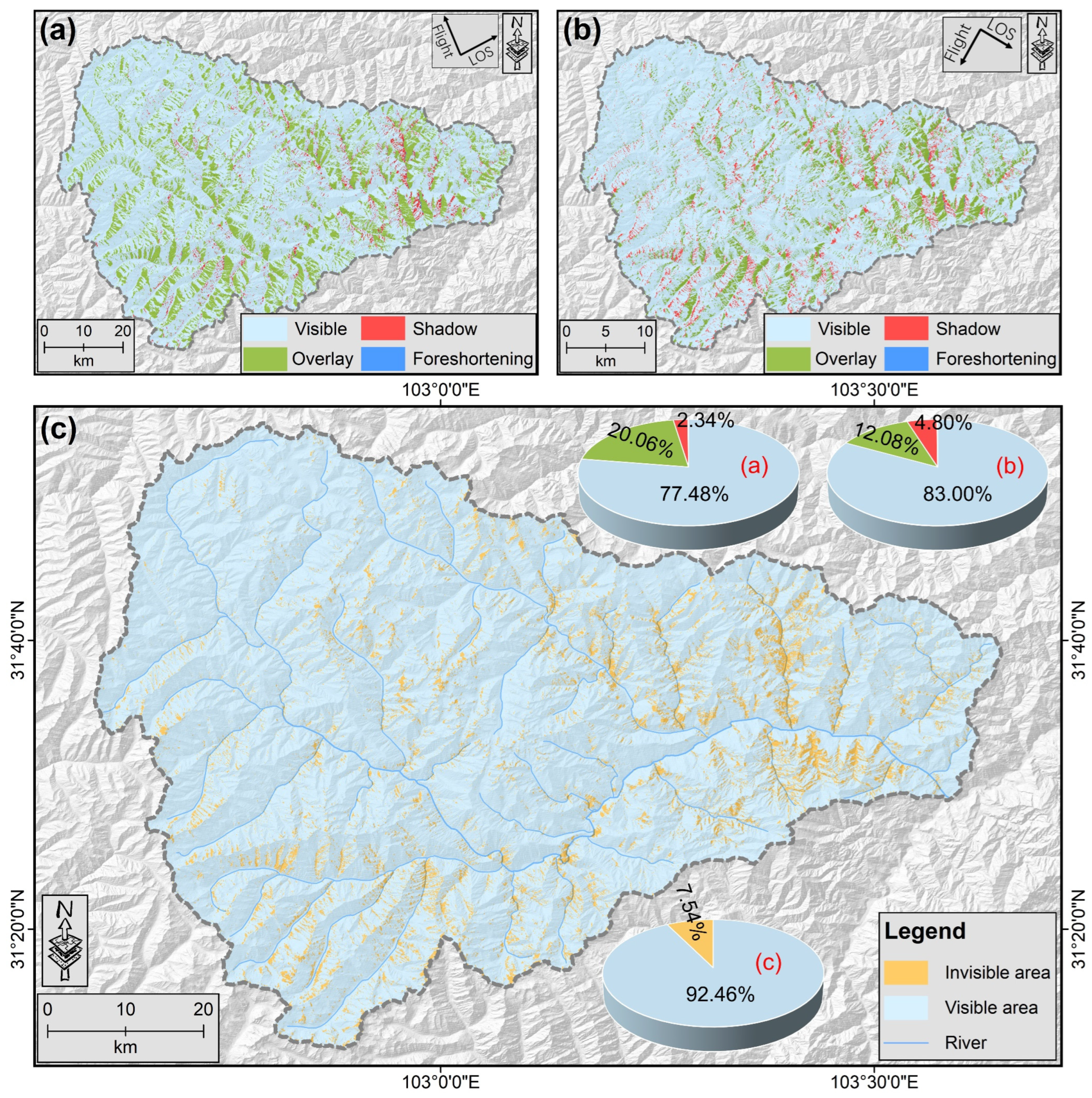
Changes in terrain affect the sequence of SAR signals reaching the imaging system, leading to geometric abnormalities such as foreshortening, shadow, and layover in SAR images. Therefore, a visibility analysis of SAR data is necessary, categorizing it into visible, shadow, layover, and foreshortening. The results indicated that the visible area for ascending data was 77.48% (Figure 14a), 83.9% for descending data (Figure 14b), and the combined visibility area for both ascending and descending data reached 92.46% (Figure 14c). Invisible areas were primarily characterized by layover and shadow.
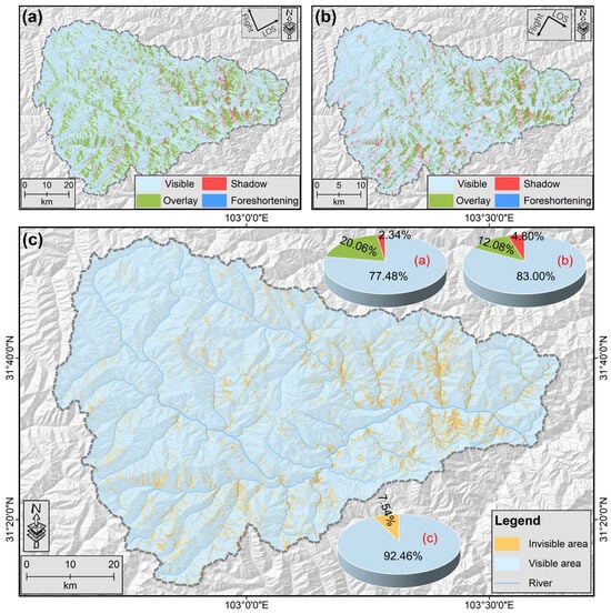
Figure 14.
Visibility evaluation maps: (a) results of the assessment of ascending data; (b) results of the assessment of descending data; (c) combined results of ascending and descending data; the colors of the pie charts a, b, c correspond to the legends of the (a–c).
The SAR satellites flew in a northward or southward direction for side-looking observations. Despite the combined visibility area exceeding 90% after combining ascending and descending data (Figure 14c), there was still some slope information in the east–west direction that remained unobserved. This deficiency was evident in the lower correlation between conditioning factors and landslides, particularly in the east and west directions (Figure 7c). This may be due to the fact that some of the east–west landslides were not fully detected. In addition, some details confirmed this shortcoming; for instance, the western steep slope of landslide A was affected by layover, while the eastern one was influenced by shadow (Figure 13b).
5.2. Comparison with Previous Study
This study improved on ref. [38]. For the landslide susceptibility assessment, ref. [38] used the neural network method, while we chose the random forest method. Both methods are recognized landslide-susceptibility assessment methods, and each has advantages and disadvantages. In terms of deformation rate classification, ref. [38] directly used 2 mm/month to classify the results without considering the study area, while we used the natural breaks method, fully considering the condition of the data study area. Unlike ref. [38], which considered rainfall data for the landslide hazard assessment, we did not. We believe that surface deformation is the main factor leading to landslides, and the InSAR technology can provide accurate and detailed information on surface deformation, so we chose to rely on InSAR data for a more accurate hazard assessment. Since rainfall data may be difficult to obtain or not accurate enough, and the deformation data provided by InSAR may be more reliable and comprehensive, we used surface deformation for the landslide hazard analysis without considering rainfall data.
Overall, we simplified and improved the landslide hazard assessment methods of ref. [38] with excellent results. This may provide a faster and simpler process for future landslide hazard assessment.
5.3. Limits and Prospect
The current study has some limitations. This research relied on InSAR technology, UAVs, airborne LiDAR, field investigations, historical optical satellite imagery, and other methods to detect landslides in the Zagunao River basin, aiming to identify every landslide and compile a comprehensive landslide inventory. However, the landslide inventory we compiled still has some shortcomings.
With the improvement in SAR image quality, the use of spaceborne InSAR for time-series observations of critical slopes or identifications of large-scale active landslides has gradually become common [18]. This study incorporated deformation information obtained from InSAR into landslide hazard assessments, aiming to ensure the completeness of deformation data. However, these data are unavoidably influenced by complicated atmospheric disturbances [64], vegetation [65], and terrain undulations [66], leading to issues such as atmospheric delays, geometric distortions, and decorrelation in the obtained results. This highlights the need to enhance the processing capabilities of InSAR technology to reduce interference.
The method proposed in this research for assessing landslide hazards can also facilitate the dynamic assessment of landslide hazards. Using InSAR technology, deformation rates of the Earth’s surface can be obtained for different periods, and when combined with landslide susceptibility maps, they can yield assessments of landslide hazards for different periods. Based on the dynamic assessment results, appropriate preventative and control measures can be applied. However, due to variations in vegetation cover over different periods, the quality of the deformation results may suffer from significant decorrelation. Therefore, using multiple SAR satellite data may enhance the accuracy of the results. Assessments of landslide hazards are the foundation for risk management, and reliable assessment outcomes can provide more scientifically sound technical support to disaster management authorities.
It is important to note that the method proposed in this paper does not consider the vulnerability of people and buildings. Areas identified as high hazard may not necessarily have any human habitation or infrastructure, which can diminish the practical impact of the assessment results. Therefore, in future studies, it may be advantageous to evaluate the vulnerability of human activities and infrastructure distribution within the study region to better serve management authorities.
6. Conclusions
This study proposed a novel method for landslide hazard assessment that combined surface deformation rates obtained from SAR data in different orbits with landslide susceptibility maps to obtain the distribution of landslide hazard levels within a specific period in the study area. This method considered not only the stability of existing landslides but also the potential reactivation and formation of new landslides, thereby improving the accuracy and practicality of the landslide hazard assessment. Using the Zagunao River basin as an example, the following main conclusions were drawn:
- (1)
- An updated landslide inventory of the Zagunao River basin was mapped using various techniques including stacking-InSAR, historical optical satellite imagery, and field investigations. Through field investigations, 26 landslides were confirmed from ascending orbit SAR data, 31 landslides from descending orbit SAR data, and 8 landslides were detected in both datasets. Additionally, by referencing a historical landslide database, 79 landslides were successfully identified using historical optical images. A landslide inventory map of 128 landslides was eventually developed.
- (2)
- Based on the landslide inventory, nine evaluation factors were selected, and a frequency ratio model was used to investigate the spatial relationships between landslides and these factors. A landslide susceptibility map for the Zagunao River basin was generated using a random forest algorithm. The results indicated that the high- and very high susceptibility zones covered 3.28% of the study area, primarily concentrated on both sides of the main stem of the Zagunao River.
- (3)
- Based on the landslide susceptibility results, a landslide hazard map was developed for the Zagunao River basin, taking into consideration the surface deformation information. Compared with previous studies, the process of landslide hazard assessment was simplified, and reliable results were obtained.
This landslide hazard assessment method uses InSAR technology to monitor surface deformation in landslide-prone areas in real time, which provides a scientific basis for landslide prevention and control. However, when using SAR data to obtain surface deformation information, the geometry effect of SAR needs to be considered, which may affect the observation results. In future landslide hazard assessments, the surface deformation rate in multiple periods can be considered to achieve a dynamic evolution process of landslide hazard.
Author Contributions
Conceptualization, Y.S. and W.L.; methodology, Y.S., W.L. and Z.X.; software, Y.S., Z.X. and S.Z.; validation, W.L. and H.L.; formal analysis, Y.S., W.L. and S.Z.; investigation, Z.X., W.Y., Z.L., X.C., P.L. and W.L.; resources, W.L.; data curation, Y.S. and Z.X.; writing—original draft preparation, Y.S.; writing—review and editing, Y.S. and W.L.; visualization, Y.S.; supervision, W.L.; project administration, W.L.; funding acquisition, W.L. All authors have read and agreed to the published version of the manuscript.
Funding
This research was funded by National Key Research and Development Program of China (2021YFC3000401), the National Key Research and the National Natural Science Foundation of China (grant No. 41941019), the Key Research and Development Program of Sichuan Province (grant No. 2023YFS0435), the Yangtze River Joint Research Phase II Program (grant No. 2022-LHYJ-02-0201), the China Power Construction Group Research Project (grant No. DJ-ZDXM-2020-3), and the State Key Laboratory of Geohazard Prevention and Geoenvironment Protection Independent Research Project (grant No. SKLGP2022Z007).
Data Availability Statement
The datasets generated and/or analyzed during the current study are available from the corresponding author upon reasonable request. The data are not publicly available due to confidentiality reasons.
Acknowledgments
Thanks to ESA for providing the Sentinel-1A images.
Conflicts of Interest
The Author Xiong Cao was employed by the Southwest Branch of China Petroleum Engineering Construction Co., Ltd., the Author Pengfei Li was employed by the Guiyang Engineering Corporation Limited of Power China. The remaining authors declare that the research was conducted in the absence of any commercial or financial relationships that could be construed as a potential conflict of interest. The funders had no role in the design of the study; in the collection, analyses, or interpretation of data; in the writing of the manuscript; or in the decision to publish the results.
References
- Chen, M.; Lv, P.; Zhang, S.; Chen, X.; Zhou, J. Time evolution and spatial accumulation of progressive failure for Xinhua slope in the Dagangshan reservoir, Southwest China. Landslides 2018, 15, 565–580. [Google Scholar] [CrossRef]
- Huang, R. Understanding the Mechanism of Large-Scale Landslides. In Engineering Geology for Society and Territory—Volume 2; Springer: Cham, Switzerland, 2015; pp. 13–32. [Google Scholar]
- Zaruba, Q.; Mencl, V. Landslides and Their Control; Elsevier: Amsterdam, The Netherlands, 2014. [Google Scholar]
- Li, Y.; Wang, X.; Mao, H. Influence of human activity on landslide susceptibility development in the Three Gorges area. Nat. Hazard. 2020, 104, 2115–2151. [Google Scholar] [CrossRef]
- Zeng, T.; Guo, Z.; Wang, L.; Jin, B.; Wu, F.; Guo, R. Tempo-Spatial Landslide Susceptibility Assessment from the Perspective of Human Engineering Activity. Remote Sens. 2023, 15, 4111. [Google Scholar] [CrossRef]
- Zhao, B.; Yuan, L.; Geng, X.; Su, L.; Qian, J.; Wu, H.; Liu, M.; Li, J. Deformation characteristics of a large landslide reactivated by human activity in Wanyuan city, Sichuan Province, China. Landslides 2022, 19, 1131–1141. [Google Scholar] [CrossRef]
- Fan, X.; Scaringi, G.; Korup, O.; West, A.J.; van Westen, C.J.; Tanyas, H.; Hovius, N.; Hales, T.C.; Jibson, R.W.; Allstadt, K.E.; et al. Earthquake-Induced Chains of Geologic Hazards: Patterns, Mechanisms, and Impacts. Rev. Geophys. 2019, 57, 421–503. [Google Scholar] [CrossRef]
- Ma, S.; Shao, X.; Xu, C. Landslides Triggered by the 2016 Heavy Rainfall Event in Sanming, Fujian Province: Distribution Pattern Analysis and Spatio-Temporal Susceptibility Assessment. Remote Sens. 2023, 15, 2738. [Google Scholar] [CrossRef]
- Li, C.; Ma, T.; Zhu, X.; Li, W. The power–law relationship between landslide occurrence and rainfall level. Geomorphology 2011, 130, 221–229. [Google Scholar] [CrossRef]
- Pardeshi, S.D.; Autade, S.E.; Pardeshi, S.S. Landslide hazard assessment: Recent trends and techniques. SpringerPlus 2013, 2, 523. [Google Scholar] [CrossRef]
- Natural Disasters. Available online: https://ourworldindata.org/natural-disasters (accessed on 22 May 2023).
- Varnes, D.; IAEG. Landslide Hazard Zonation: A Review of Principles and Practice; United Nations Scientific and Cultural Organization: Paris, France, 1984; pp. 1–6. [Google Scholar]
- Wang, Y.; Wen, H.; Sun, D.; Li, Y. Quantitative Assessment of Landslide Risk Based on Susceptibility Mapping Using Random Forest and GeoDetector. Remote Sens. 2021, 13, 2625. [Google Scholar] [CrossRef]
- Thiery, Y.; Terrier, M.; Colas, B.; Fressard, M.; Maquaire, O.; Grandjean, G.; Gourdier, S. Improvement of landslide hazard assessments for regulatory zoning in France: STATE–OF–THE-ART perspectives and considerations. Int. J. Disaster Risk Reduct. 2020, 47, 101562. [Google Scholar] [CrossRef]
- Jaiswal, A.; Verma, A.K.; Singh, T.N.; Singh, J. Landslide Hazard Assessment Using Machine Learning and GIS. In Landslides: Detection, Prediction and Monitoring: Technological Developments; Thambidurai, P., Singh, T.N., Eds.; Springer International Publishing: Cham, Switzerland, 2023; pp. 383–399. [Google Scholar]
- Esposito, C.; Mastrantoni, G.; Marmoni, G.M.; Antonielli, B.; Caprari, P.; Pica, A.; Schilirò, L.; Mazzanti, P.; Bozzano, F. From theory to practice: Optimisation of available information for landslide hazard assessment in Rome relying on official, fragmented data sources. Landslides 2023, 20, 2055–2073. [Google Scholar] [CrossRef]
- Colombo, A.; Lanteri, L.; Ramasco, M.; Troisi, C. Systematic GIS-based landslide inventory as the first step for effective landslide-hazard management. Landslides 2005, 2, 291–301. [Google Scholar] [CrossRef]
- Xu, Q.; Zhao, B.; Dai, K.; Dong, X.; Li, W.; Zhu, X.; Yang, Y.; Xiao, X.; Wang, X.; Huang, J.; et al. Remote sensing for landslide investigations: A progress report from China. Eng. Geol. 2023, 321, 107156. [Google Scholar] [CrossRef]
- Lee, C.-F.; Singhroy, V.; Lin, S.-Y.; Huang, W.-K.; Li, J. Landslide Activity Assessment of a Subtropical Area by Integrating InSAR, Landslide Inventory, Airborne LiDAR, and UAV Investigations: A Case Study in Northern Taiwan. In Advances in Remote Sensing for Infrastructure Monitoring; Singhroy, V., Ed.; Springer International Publishing: Cham, Switzerland, 2021; pp. 111–136. [Google Scholar]
- Tang, H.; Wang, C.; An, S.; Wang, Q.; Jiang, C. A Novel Heterogeneous Ensemble Framework Based on Machine Learning Models for Shallow Landslide Susceptibility Mapping. Remote Sens. 2023, 15, 4159. [Google Scholar] [CrossRef]
- Huang, F.; Cao, Z.; Guo, J.; Jiang, S.-H.; Li, S.; Guo, Z. Comparisons of heuristic, general statistical and machine learning models for landslide susceptibility prediction and mapping. CATENA 2020, 191, 104580. [Google Scholar] [CrossRef]
- Xie, W.; Nie, W.; Saffari, P.; Robledo, L.F.; Descote, P.-Y.; Jian, W. Landslide hazard assessment based on Bayesian optimization–support vector machine in Nanping City, China. Nat. Hazard. 2021, 109, 931–948. [Google Scholar] [CrossRef]
- Shahabi, H.; Ahmadi, R.; Alizadeh, M.; Hashim, M.; Al-Ansari, N.; Shirzadi, A.; Wolf, I.D.; Ariffin, E.H. Landslide Susceptibility Mapping in a Mountainous Area Using Machine Learning Algorithms. Remote Sens. 2023, 15, 3112. [Google Scholar] [CrossRef]
- Parise, M. Landslide hazard zonation of slopes susceptible to rock falls and topples. Nat. Hazards Earth Syst. Sci. 2002, 2, 37–49. [Google Scholar] [CrossRef]
- Preuth, T.; Glade, T.; Demoulin, A. Stability analysis of a human-influenced landslide in eastern Belgium. Geomorphology 2010, 120, 38–47. [Google Scholar] [CrossRef]
- Materazzi, M.; Bufalini, M.; Gentilucci, M.; Pambianchi, G.; Aringoli, D.; Farabollini, P. Landslide Hazard Assessment in a Monoclinal Setting (Central Italy): Numerical vs. Geomorphological Approach. Land 2021, 10, 624. [Google Scholar] [CrossRef]
- Vandromme, R.; Thiery, Y.; Bernardie, S.; Sedan, O. ALICE (Assessment of Landslides Induced by Climatic Events): A single tool to integrate shallow and deep landslides for susceptibility and hazard assessment. Geomorphology 2020, 367, 107307. [Google Scholar] [CrossRef]
- Nakileza, B.R.; Nedala, S. Topographic influence on landslides characteristics and implication for risk management in upper Manafwa catchment, Mt Elgon Uganda. Geoenviron. Disasters 2020, 7, 27. [Google Scholar] [CrossRef]
- Kamal, A.S.M.M.; Hossain, F.; Ahmed, B.; Rahman, M.Z.; Sammonds, P. Assessing the effectiveness of landslide slope stability by analysing structural mitigation measures and community risk perception. Nat. Hazard. 2023, 117, 2393–2418. [Google Scholar] [CrossRef]
- Sim, K.B.; Lee, M.L.; Wong, S.Y. A review of landslide acceptable risk and tolerable risk. Geoenviron. Disasters 2022, 9, 3. [Google Scholar] [CrossRef]
- Crozier, M.J.; Glade, T. Landslide Hazard and Risk: Issues, Concepts and Approach; Glade, T., Anderson, M., Crozier, M., Eds.; Wiley: Chichester, UK, 2005; pp. 1–40. [Google Scholar]
- Curlander, J.C.; McDonough, R.N. Synthetic Aperture Radar; Wiley: New York, NY, USA, 1991; Volume 11. [Google Scholar]
- Zebker, H.A.; Goldstein, R.M. Topographic mapping from interferometric synthetic aperture radar observations. J. Geophys. Res. Solid Earth 1986, 91, 4993–4999. [Google Scholar] [CrossRef]
- Ferretti, A.; Prati, C.; Rocca, F. Permanent scatterers in SAR interferometry. IEEE Trans. Geosci. Remote Sens. 2001, 39, 8–20. [Google Scholar] [CrossRef]
- Zhou, C.; Cao, Y.; Hu, X.; Yin, K.; Wang, Y.; Catani, F. Enhanced dynamic landslide hazard mapping using MT-InSAR method in the Three Gorges Reservoir Area. Landslides 2022, 19, 1585–1597. [Google Scholar] [CrossRef]
- Ciampalini, A.; Raspini, F.; Lagomarsino, D.; Catani, F.; Casagli, N. Landslide susceptibility map refinement using PSInSAR data. Remote Sens. Environ. 2016, 184, 302–315. [Google Scholar] [CrossRef]
- He, Y.; Wang, W.; Zhang, L.; Chen, Y.; Chen, Y.; Chen, B.; He, X.; Zhao, Z. An identification method of potential landslide zones using InSAR data and landslide susceptibility. Geomat. Nat. Hazards Risk 2023, 14, 2185120. [Google Scholar] [CrossRef]
- Dai, C.; Li, W.; Lu, H.; Zhang, S. Landslide Hazard Assessment Method Considering the Deformation Factor: A Case Study of Zhouqu, Gansu Province, Northwest China. Remote Sens. 2023, 15, 596. [Google Scholar] [CrossRef]
- Berardino, P.; Fornaro, G.; Lanari, R.; Sansosti, E. A new algorithm for surface deformation monitoring based on small baseline differential SAR interferograms. IEEE Trans. Geosci. Remote Sens. 2002, 40, 2375–2383. [Google Scholar] [CrossRef]
- Liu, W.; Zhang, Y.; Liang, Y.; Sun, P.; Li, Y.; Su, X.; Wang, A.; Meng, X. Landslide Risk Assessment Using a Combined Approach Based on InSAR and Random Forest. Remote Sens. 2022, 14, 2131. [Google Scholar] [CrossRef]
- Lin, Y.; Wen, H.; Liu, S. Surface runoff response to climate change based on artificial neural network (ANN) models: A case study with Zagunao catchment in Upper Minjiang River, Southwest China. J. Water Clim. Change 2018, 10, 158–166. [Google Scholar] [CrossRef]
- Zhou, C.; Yin, K.; Cao, Y.; Ahmed, B.; Li, Y.; Catani, F.; Pourghasemi, H.R. Landslide susceptibility modeling applying machine learning methods: A case study from Longju in the Three Gorges Reservoir area, China. Comput. Geosci. 2018, 112, 23–37. [Google Scholar] [CrossRef]
- Guzzetti, F.; Mondini, A.C.; Cardinali, M.; Fiorucci, F.; Santangelo, M.; Chang, K.-T. Landslide inventory maps: New tools for an old problem. Earth Sci. Rev. 2012, 112, 42–66. [Google Scholar] [CrossRef]
- Hong, H.; Pourghasemi, H.R.; Pourtaghi, Z.S. Landslide susceptibility assessment in Lianhua County (China): A comparison between a random forest data mining technique and bivariate and multivariate statistical models. Geomorphology 2016, 259, 105–118. [Google Scholar] [CrossRef]
- Ayalew, L.; Yamagishi, H. The application of GIS-based logistic regression for landslide susceptibility mapping in the Kakuda-Yahiko Mountains, Central Japan. Geomorphology 2005, 65, 15–31. [Google Scholar] [CrossRef]
- Süzen, M.L.; Kaya, B.Ş. Evaluation of environmental parameters in logistic regression models for landslide susceptibility mapping. Int. J. Digit. Earth 2012, 5, 338–355. [Google Scholar] [CrossRef]
- Xu, C.; Xu, X.; Wu, X.; Dai, F.; Yao, X.; Yao, Q. Etailed catalog of landslides triggered by the 2008 wen chuan earthquake and statistical analyses of their spa tial distribution. J. Eng. Geol. 2013, 21, 25–44. (In Chinese) [Google Scholar]
- Deng, H.; He, Z.; Chen, Y.; Cai, H.; Li, X. Application of information quantity model to hazard evaluation of geological disaster in mountainous region environment: A case study of Luding County, Sichuan Province. J. Nat. Disasters 2014, 23, 67–76. (In Chinese) [Google Scholar]
- Peduzzi, P. Landslides and vegetation cover in the 2005 North Pakistan earthquake: A GIS and statistical quantitative approach. Nat. Hazards Earth Syst. Sci. 2010, 10, 623–640. [Google Scholar] [CrossRef]
- Shan, Y.; Dai, X.; Li, W.; Yang, Z.; Wang, Y.; Qu, G.; Liu, W.; Ren, J.; Li, C.; Liang, S.; et al. Detecting Spatial-Temporal Changes of Urban Environment Quality by Remote Sensing-Based Ecological Indices: A Case Study in Panzhihua City, Sichuan Province, China. Remote Sens. 2022, 14, 4137. [Google Scholar] [CrossRef]
- Pacheco Quevedo, R.; Velastegui-Montoya, A.; Montalván-Burbano, N.; Morante-Carballo, F.; Korup, O.; Daleles Rennó, C. Land use and land cover as a conditioning factor in landslide susceptibility: A literature review. Landslides 2023, 20, 967–982. [Google Scholar] [CrossRef]
- Zhang, T.; Han, L.; Han, J.; Li, X.; Zhang, H.; Wang, H. Assessment of Landslide Susceptibility Using Integrated Ensemble Fractal Dimension with Kernel Logistic Regression Model. Entropy 2019, 21, 218. [Google Scholar] [CrossRef] [PubMed]
- Lee, S.; Pradhan, B. Landslide hazard mapping at Selangor, Malaysia using frequency ratio and logistic regression models. Landslides 2007, 4, 33–41. [Google Scholar] [CrossRef]
- Pudlo, P.; Marin, J.-M.; Estoup, A.; Cornuet, J.-M.; Gautier, M.; Robert, C.P. Reliable ABC model choice via random forests. Bioinformatics 2016, 32, 859–866. [Google Scholar] [CrossRef] [PubMed]
- Breiman, L. Random Forests. Mach. Learn. 2001, 45, 5–32. [Google Scholar] [CrossRef]
- Kohestani, V.R.; Hassanlourad, M.; Ardakani, A. Evaluation of liquefaction potential based on CPT data using random forest. Nat. Hazard. 2015, 79, 1079–1089. [Google Scholar] [CrossRef]
- Trigila, A.; Iadanza, C.; Esposito, C.; Scarascia-Mugnozza, G. Comparison of Logistic Regression and Random Forests techniques for shallow landslide susceptibility assessment in Giampilieri (NE Sicily, Italy). Geomorphology 2015, 249, 119–136. [Google Scholar] [CrossRef]
- Wu, H.; Nian, T.K.; Shan, Z.G. Investigation of landslide dam life span using prediction models based on multiple machine learning algorithms. Geomat. Nat. Hazards Risk 2023, 14, 2273213. [Google Scholar] [CrossRef]
- He, Q.; Shahabi, H.; Shirzadi, A.; Li, S.; Chen, W.; Wang, N.; Chai, H.; Bian, H.; Ma, J.; Chen, Y.; et al. Landslide spatial modelling using novel bivariate statistical based Naïve Bayes, RBF Classifier, and RBF Network machine learning algorithms. Sci. Total Environ. 2019, 663, 1–15. [Google Scholar] [CrossRef]
- Stumpf, A.; Kerle, N. Object-oriented mapping of landslides using Random Forests. Remote Sens. Environ. 2011, 115, 2564–2577. [Google Scholar] [CrossRef]
- Guo, R. Subject: Assessment of Landslide Susceptibility Based on Ensemble Learning Algorithm in Xi’an City. Master’s Thesis, Xi’an University of Science and Technology, Xi’an, China, 2021. [Google Scholar]
- Maltman, A. The Geological Deformation of Sediments; Springer Science & Business Media: Berlin/Heidelberg, Germany, 2012. [Google Scholar]
- Fawcett, T. An introduction to ROC analysis. Pattern Recognit. Lett. 2006, 27, 861–874. [Google Scholar] [CrossRef]
- Zhao, L.; Liang, R.; Shi, X.; Dai, K.; Cheng, J.; Cao, J. Detecting and Analyzing the Displacement of a Small-Magnitude Earthquake Cluster in Rong County, China by the GACOS Based InSAR Technology. Remote Sens. 2021, 13, 4137. [Google Scholar] [CrossRef]
- Yan, Z.; Yan, H.; Wang, T. A fast non-local means filtering method for interferometric phase based on wavelet packet transform. Radio Sci. 2021, 56, e2019RS007052. [Google Scholar] [CrossRef]
- Colesanti, C.; Wasowski, J. Investigating landslides with space-borne Synthetic Aperture Radar (SAR) interferometry. Eng. Geol. 2006, 88, 173–199. [Google Scholar] [CrossRef]


Disclaimer/Publisher’s Note: The statements, opinions and data contained in all publications are solely those of the individual author(s) and contributor(s) and not of MDPI and/or the editor(s). MDPI and/or the editor(s) disclaim responsibility for any injury to people or property resulting from any ideas, methods, instructions or products referred to in the content. |
© 2023 by the authors. Licensee MDPI, Basel, Switzerland. This article is an open access article distributed under the terms and conditions of the Creative Commons Attribution (CC BY) license (https://creativecommons.org/licenses/by/4.0/).