
Sub-Hourly Variations of Wind Shear in the Mesosphere-Lower Thermosphere as Observed by the China Meteor Radar Chain
 , and
, and 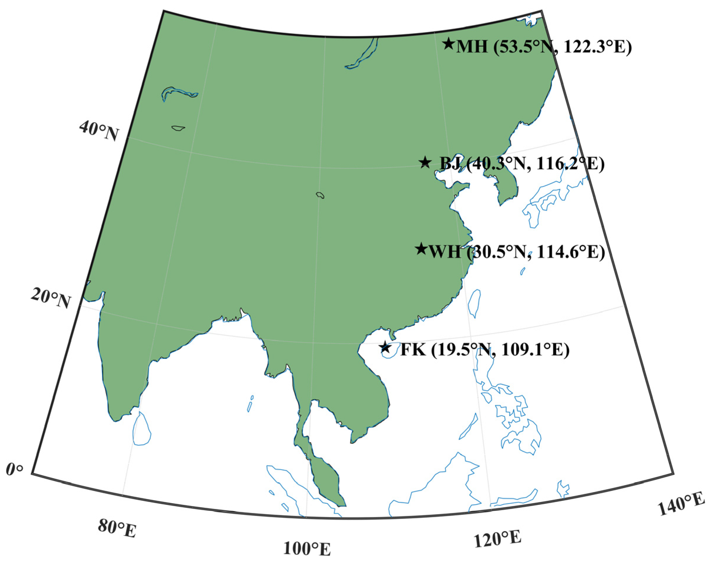
Abstract
:1. Introduction
2. Data and Methods
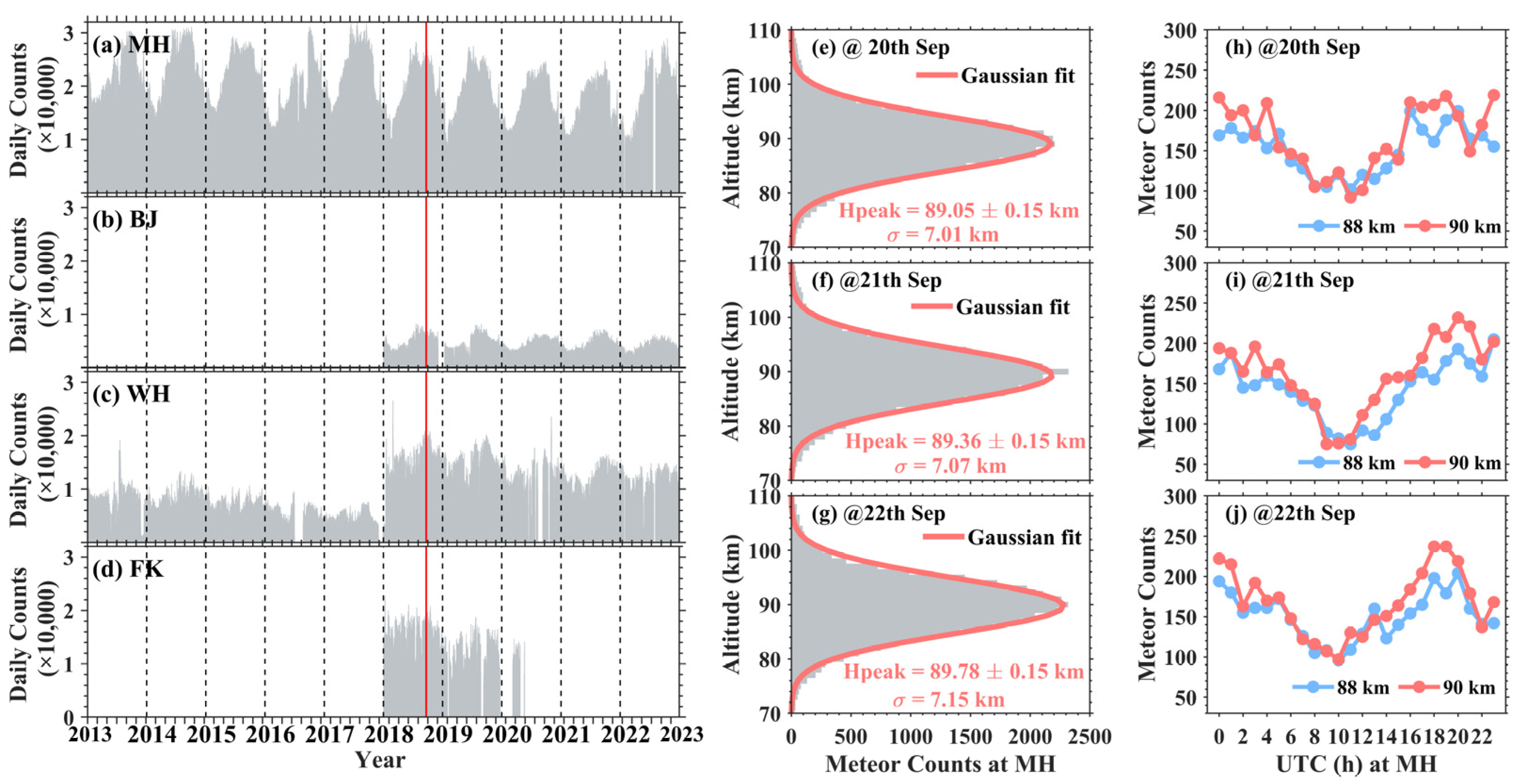
2.1. Meteor Data Description
2.2. The Traditional Method: Least Square Algorithm (LSA)
2.3. The Newly Proposed Method: Damped Least Square Algorithm (DLSA)
2.4. Estimating the Error of Meteor Wind
2.5. Method for Evaluating the Quality of the Inversion of Wind
2.6. Calculating Wind Shear S
2.7. GW Kinetic Energy in the MLT Region
3. Results
4. Conclusions
Author Contributions
Funding
Data Availability Statement
Conflicts of Interest
References
- Dong, W.; Fritts, D.C.; Liu, A.Z.; Lund, T.S.; Liu, H.-L. Gravity waves emitted from Kelvin-Helmholtz instabilities. Geophys. Res. Lett. 2023, 50, e2022GL102674. [Google Scholar] [CrossRef]
- Fritts, D.C.; Alexander, M.J. Gravity wave dynamics and effects in the middle atmosphere. Rev. Geophys. 2003, 41, L09801. [Google Scholar] [CrossRef]
- Shao, J.; Zhang, J.; Tian, Y.; Wang, W.; Huang, K.; Zhang, S. Tropospheric gravity waves increase the likelihood of double tropopauses. Geophys. Res. Lett. 2023, 50, e2023GL105724. [Google Scholar] [CrossRef]
- Shutts, G.J.; Kitchen, M.; Hoare, P.H. A large amplitude gravity wave in the lower stratosphere detected by radiosonde. Q. J. R. Meteorol. Soc. 1988, 114, 579–594. [Google Scholar] [CrossRef]
- Kitchen, M.; Shutts, G.J. Radiosonde observations of large-amplitude gravity waves in the lower and middle stratosphere. J. Geophys. Res. Atmos. 1990, 95, 20451–20455. [Google Scholar] [CrossRef]
- Cadet, D.; Teitelbaum, H. Observational evidence of internal inertia-gravity waves in the tropical stratosphere. J. Atmos. Sci. 1979, 36, 892–907. [Google Scholar] [CrossRef]
- Houchi, K.; Stoffelen, A.; Marseille, G.; De Kloe, J. Comparison of wind and wind shear climatologies derived from high-resolution radiosondes and the ECMWF model. J. Geophys. Res. Atmos. 2010, 115, D22123. [Google Scholar] [CrossRef]
- Einaudi, F.; Lalas, D.P.; Perona, G. The role of gravity waves in tropospheric processes. Pure Appl. Geophys. 1978, 117, 627–663. [Google Scholar] [CrossRef]
- Fritts, D.C. Gravity wave saturation in the middle atmosphere: A review of theory and observations. Rev. Geophys. 1984, 22, 275–308. [Google Scholar] [CrossRef]
- Baumgarten, G.; Fritts, D.C. Quantifying Kelvin-Helmholtz instability dynamics observed in noctilucent clouds: 1. Methods and observations. J. Geophys. Res. Atmos. 2014, 119, 9324–9337. [Google Scholar] [CrossRef]
- Chau, J.L.; Urco, J.M.; Avsarkisov, V.; Vierinen, J.P.; Latteck, R.; Hall, C.M.; Tsutsumi, M. Four-dimensional quantification of Kelvin-Helmholtz instabilities in the polar summer mesosphere using volumetric radar imaging. Geophys. Res. Lett. 2020, 47, e2019GL086081. [Google Scholar] [CrossRef]
- Fritts, D.; Rastogi, P. Convective and dynamical instabilities due to gravity wave motions in the lower and middle atmosphere: Theory and observations. Radio Sci. 1985, 20, 1247–1277. [Google Scholar] [CrossRef]
- Layzer, D. The turbulence criteria in stably stratified shear flow and the origin of sporadic E. In Ionospheric Sporadic E; Smith, E.K., Matsushita, S., Eds.; Macmillan: New York, NY, USA, 1962; pp. 258–275. [Google Scholar] [CrossRef]
- Smith, L.G.; Miller, K.L. Sporadic-E layers and unstable wind shears. J. Atmos. Terr. Phys. 1980, 42, 45–50. [Google Scholar] [CrossRef]
- Larsen, M.F. A shear instability seeding mechanism for quasiperiodic radar echoes. J. Geophys. Res. Space Phys. 2000, 105, 24931–24940. [Google Scholar] [CrossRef]
- Choudhary, R.K.; St-Maurice, J.P.; Kagan, L.M.; Mahajan, K.K. Quasi-periodic backscatters from the E region at Gadanki: Evidence for Kelvin-Helmholtz billows in the lower thermosphere? J. Geophys. Res. Space Phys. 2005, 110, A08303. [Google Scholar] [CrossRef]
- Eaton, F.; Mclaughlin, S.A.; Hines, J.R. A new frequency-modulated continuous wave radar for studying planetary boundary layer morphology. Radio Sci. 1995, 30, 75–88. [Google Scholar] [CrossRef]
- Fritts, D.C.; Baumgarten, G.; Wan, K.; Werne, J.; Lund, T. Quantifying Kelvin-Helmholtz instability dynamics observed in noctilucent clouds: 2. Modeling and interpretation of observations. J. Geophys. Res. Atmos. 2014, 119, 9359–9375. [Google Scholar] [CrossRef]
- Hecht, J.H.; Wan, K.; Gelinas, L.J.; Fritts, D.C.; Walterscheid, R.L.; Rudy, R.J.; Franke, S.J.; Vargas, F.A.; Pautet, P.D.; Taylor, M.J.; et al. The life cycle of instability features measured from the Andes lidar observatory over Cerro Pachon on 24 March 2012. J. Geophys. Res. Atmos. 2014, 119, 8872–8898. [Google Scholar] [CrossRef]
- Hecht, J.H.; Fritts, D.C.; Gelinas, L.J.; Rudy, R.J.; Walterscheid, R.L.; Liu, A.Z. Kelvin-Helmholtz billow interactions and instabilities in the mesosphere over the Andes Lidar Observatory: 1. Observations. J. Geophys. Res. Atmos. 2021, 126, e2020JD033414. [Google Scholar] [CrossRef]
- Lehmacher, G.A.; Guo, L.; Kudeki, E.; Reyes, P.M.; Akgiray, A.; Chau, J.L. High-resolution observations of mesospheric layers with the Jicamarca VHF radar. Adv. Space Res. 2007, 40, 734–743. [Google Scholar] [CrossRef]
- Pfrommer, T.; Hickson, P.; She, C.-Y. A large-aperture sodium fluorescence lidar with very high resolution for mesopause dynamics and adaptive optics studies. Geophys. Res. Lett. 2009, 35, L15831. [Google Scholar] [CrossRef]
- Fritts, D.C.; Wang, L.; Lund, T.S.; Thorpe, S.A.; Kjellstrand, C.B.; Kaifler, B.; Kaifler, N. Multi-Scale Kelvin-Helmholtz instability dynamics observed by PMC Turbo on 12 July 2018: 2. DNS modeling of KHI dynamics and PMC responses. J. Geophys. Res. Atmos. 2022, 127, e2021JD035834. [Google Scholar] [CrossRef]
- Sharman, R.D.; Trier, S.B.; Lane, T.P.; Doyle, J.D. Sources and dynamics of turbulence in the upper troposphere and lower stratosphere: A review. Geophys. Res. Lett. 2012, 39, L12803. [Google Scholar] [CrossRef]
- Ko, H.C.; Chun, H.Y. Potential sources of atmospheric turbulence estimated using the Thorpe method and operational radiosonde data in the United States. Atmos. Res. 2022, 265, 105891. [Google Scholar] [CrossRef]
- Ko, H.C.; Chun, H.Y.; Wilson, R.; Geller, M.A. Characteristics of atmospheric turbulence retrieved from high vertical-resolution radiosonde data in the United States. J. Geophys. Res.-Atmos. 2019, 124, 7553–7579. [Google Scholar] [CrossRef]
- Shao, J.; Zhang, J.; Wang, W.; Zhang, S.; Yu, T.; Dong, W. Occurrence frequency of subcritical Richardson numbers assessed by global high-resolution radiosonde and ERA5 reanalysis. Atmos. Chem. Phys. 2023, 23, 12589–12607. [Google Scholar] [CrossRef]
- Alexander, M.J.; Tsuda, T.; Vincent, R.A. Latitudinal variations observed in gravity waves with short vertical wavelengths. J. Atmos. Sci. 2002, 59, 1394–1404. [Google Scholar] [CrossRef]
- Hickey, M.P.; Taylor, M.J.; Gardner, C.S.; Gibbons, C.R. Full-wave modeling of small-scale gravity waves using Airborne Lidar and Observations of the Hawaiian Airglow (ALOHA-93) O (1 S) images and coincident Na wind/temperature lidar measurements. J. Geophys. Res. Atmos. 1998, 103, 6439–6453. [Google Scholar] [CrossRef]
- Taylor, M.J.; Pendleton, W.R., Jr.; Clark, S.; Takahashi, H.; Gobbi, D.; Goldberg, R.A. Image measurements of short-period gravity waves at equatorial latitudes. J. Geophys. Res. Atmos. 1997, 102, 26283–26299. [Google Scholar] [CrossRef]
- McLandress, C.; Alexander, M.J.; Wu, D.L. Microwave Limb Sounder observations of gravity waves in the stratosphere: A climatology and interpretation. J. Geophys. Res. Atmos. 2000, 105, 11947–11967. [Google Scholar] [CrossRef]
- Dewan, E.M.; Picard, R.H.; O’Neil, R.R.; Gardiner, H.A.; Gibson, J.; Mill, J.D.; Richards, E.; Kendra, M.; Gallery, W.O. MSX satellite observations of thunderstorm-generated gravity waves in mid-wave infrared images of the upper stratosphere. Geophys. Res. Lett. 1998, 25, 939–942. [Google Scholar] [CrossRef]
- Fritts, D.C.; Wang, D.Y. Doppler-shifting effects on frequency spectra of gravity waves observed near the summer mesopause at high latitude. J. Atmos. Sci. 1991, 48, 1535–1544. [Google Scholar] [CrossRef]
- Hoppe, U.P.; Fritts, D.C. High-resolution measurements of vertical velocity with the European incoherent scatter VHF radar: 1. Motion field characteristics and measurement biases. J. Geophys. Res. Atmos. 1995, 100, 16813–16825. [Google Scholar] [CrossRef]
- Blumen, W.; Banta, R.; Burns, S.P.; Fritts, D.C.; Newsom, R.; Poulos, G.S.; Sun, J. Turbulence statistics of a Kelvin–Helmholtz billow event observed in the nighttime boundary layer during the Cooperative Atmosphere–Surface Exchange Study field program. Dyn. Atmos. Ocean. 2001, 34, 189–204. [Google Scholar] [CrossRef]
- Chapman, D.; Browning, K.A. Radar observations of wind-shear splitting within evolving atmospheric Kelvin-Helmholtz billows. Q. J. R. Meteorol. Soc. 1997, 123, 1433–1439. [Google Scholar] [CrossRef]
- Hecht, J.H. Instability layers and airglow imaging. Rev. Geophys. 2004, 42, RG1001. [Google Scholar] [CrossRef]
- Luce, H.; Hassenpflug, G.; Yamamoto, M.; Fukao, S.; Sato, K. High-resolution observations with MU radar of a KH instability triggered by an inertia-gravity wave in the upper part of a Jet-Stream. J. Atmos. Sci. 2008, 65, 1711–1718. [Google Scholar] [CrossRef]
- Liu, H.-L. Large wind shears and their implications for diffusion in regions with enhanced static stability: The mesopause and the tropopause. J. Geophys. Res. Atmos. 2017, 122, 9579–9590. [Google Scholar] [CrossRef]
- Fritts, D.C.; Wang, L.; Werne, J.A. Gravity wave–fine structure interactions. Part I: Influences of fine structure form and orientation on flow evolution and instability. J. Atmos. Sci. 2013, 70, 3710–3734. [Google Scholar] [CrossRef]
- Cao, B.; Heale, C.J.; Guo, Y.; Liu, A.Z.; Snively, J.B. Observation and modeling of gravity wave propagation through reflection and critical layers above Andes Lidar Observatory at Cerro Pachón, Chile. J. Geophys. Res. Atmos. 2016, 121, 12–737. [Google Scholar] [CrossRef]
- Liu, L.; Liu, H.; Chen, Y.; Le, H.; Sun, Y.-Y.; Ning, B.; Hu, L.; Wan, W. Variations of the meteor echo heights at Beijing and Mohe, China. J. Geophys. Res. Space Phys. 2016, 122, 1117–1127. [Google Scholar] [CrossRef]
- Yu, Y.; Wan, W.; Ning, B.; Liu, L.; Wang, Z.; Hu, L.; Ren, Z. Tidal wind mapping from observations of a meteor radar chain in December 2011. J. Geophys. Res. Space Phys. 2013, 118, 2321–2332. [Google Scholar] [CrossRef]
- Jiang, G.; Xu, J.; Shi, J.; Yang, G.; Wang, X.; Yan, C. The first observation of the atmospheric tides in the mesosphere and lower thermosphere over Hainan, China. Chin. Sci. Bull. 2010, 55, 1059–1066. [Google Scholar] [CrossRef]
- Kursinski, E.R.; Hajj, G.A.; Schofield, J.T.; Linfield, R.P.; Hardy, K.R. Observing Earth’s atmosphere with radio occultation measurements using the Global Positioning System. J. Geophys. Res. 1997, 102, 23429–23465. [Google Scholar] [CrossRef]
- He, W.; Ho, S.-P.; Chen, H.; Zhou, X.; Hunt, D.; Kuo, Y.-H. Assessment of radiosonde temperature measurements in the upper troposphere and lower stratosphere using COSMIC radio occultation data. Geophys. Res. Lett. 2009, 36, L17807. [Google Scholar] [CrossRef]
- Scherllin-Pirscher, B.; Steiner, A.K.; Anthes, R.A.; Alexander, M.J.; Alexander, S.P.; Biondi, R.; Birner, T.; Kim, J.; Randel, W.J.; Son, S.-W.; et al. Tropical temperature variability in the UTLS: New insights from GPS radio occultation observations. J. Clim. 2021, 34, 2813–2838. [Google Scholar] [CrossRef]
- Cucurull, L.; Casey, S.P.F. Improved impacts in observing system simulation experiments of radio occultation observations as a result of model and data assimilation changes. Mon. Weather Rev. 2021, 149, 207–220. [Google Scholar] [CrossRef]
- Zhang, H.; Huangfu, J.; Wang, X.; Chen, W.; Peng, W.; Tang, Q.; Chu, Y.; Xue, Z. Comparative analysis of Binhu and cosmic-2 radio occultation data. Remote Sens. 2022, 14, 4958. [Google Scholar] [CrossRef]
- Hocking, W.K.; Fuller, B.; Vandepeer, B. Real-time determination of meteor-related parameters utilizing modern digital technology. J. Atmos. Sol.—Terr. Phys. 2001, 63, 155–169. [Google Scholar] [CrossRef]
- Holdsworth, D.A.; Reid, I.M. The Buckland Park MF radar: Routine observation scheme and velocity comparisons. Ann. Geophys. 2004, 22, 3815–3828. [Google Scholar] [CrossRef]
- Holdsworth, D.A.; Reid, I.M.; Cervera, M.A. Buckland Park all-sky interferometric meteor radar. Radio Sci. 2004, 39, 1–12. [Google Scholar] [CrossRef]
- Hocking, W.K.; Thayaparan, T.; Jones, J. Meteor decay times and their use in determining a diagnostic mesospheric temperature-pressure parameter: Methodology and one year of data. Geophys. Res. Lett. 1997, 24, 2977–2980. [Google Scholar] [CrossRef]
- Hocking, W.K.; Thayaparan, T. Simultaneous and colocated observation of winds and tides by MF and meteor radars over London, Canada (43 N, 81 W), during 1994–1996. Radio Sci. 1997, 32, 833–865. [Google Scholar] [CrossRef]
- Menke, W. Geophysical Data Analysis: Discrete Inverse Theory; Academic Press: Cambridge, MA, USA, 2018. [Google Scholar] [CrossRef]
- Stober, G.; Chau, J.L.; Vierinen, J.; Jacobi, C.; Wilhelm, S. Retrieving horizontally resolved wind fields using multi-static meteor radar observations. Atmos. Meas. Tech. 2018, 11, 4891–4907. [Google Scholar] [CrossRef]
- Aster, R.C.; Borchers, B.; Thurber, C.H. Parameter Estimation and Inverse Problems; Elsevier: Amsterdam, The Netherlands, 2018. [Google Scholar] [CrossRef]
- Long, C.; Yu, T.; Sun, Y.-Y.; Yan, X.; Zhang, J.; Yang, N.; Wang, J.; Xia, C.; Liang, Y.; Ye, H. Atmospheric Gravity Wave Derived from the Neutral Wind with 5-Minute Resolution Routinely Retrieved by the Meteor Radar at Mohe. Remote Sens. 2023, 15, 296. [Google Scholar] [CrossRef]
- Andrioli, V.F.; Batista, P.P.; Xu, J.; Yang, G.; Chi, W.; Zhengkuan, L. Strong temperature gradients and vertical wind shear on MLT region associated to instability source at 23 S. J. Geophys. Res. Space Phys. 2017, 122, 4500–4511. [Google Scholar] [CrossRef]
- Rodriguez Imazio, P.; Dörnbrack, A.; Urzua, R.D.; Rivaben, N.; Godoy, A. Clear air turbulence observed across a tropopause fold over the Drake Passage—A case study. J. Geophys. Res. Atmos. 2022, 127, e2021JD035908. [Google Scholar] [CrossRef]
- Wang, L.; Geller, M.A. Morphology of gravity-wave energy as observed from 4 years (1998–2001) of high vertical resolution U.S. radiosonde data. J. Geophys. Res. 2003, 108, 4489. [Google Scholar] [CrossRef]
- Wang, L.; Geller, M.A.; Alexander, M.J. Spatial and temporal variations of gravity wave parameters, Part I: Intrinsic frequency, wavelength, and vertical propagation direction. J. Atmos. Sci. 2005, 62, 125–142. [Google Scholar] [CrossRef]
- Zhang, S.D.; Yi, F. Latitudinal and seasonal variations of inertial gravity wave activity in the lower atmosphere over central China. J. Geophys. Res. 2007, 112, D05109. [Google Scholar] [CrossRef]
- Alexander, S.P.; Klekociuk, A.R.; Murphy, D.J. Rayleigh lidar observations of gravity wave activity in the winter upper stratosphere and lower mesosphere above Davis, Antarctica (69° S, 78° E). J. Geophys. Res. Atmos. 2011, 116, 1–12. [Google Scholar] [CrossRef]
- Baumgarten, K.; Gerding, M.; Lübken, F.J. Seasonal variation of gravity wave parameters using different filter methods with daylight lidar measurements at midlatitudes. J. Geophys. Res. 2017, 122, 2683–2695. [Google Scholar] [CrossRef]
- Kopp, M.; Gerding, M.; Höffner, J.; Lübken, F.-J. Tidal signatures in temperatures derived from daylight lidar sound- ings above Kühlungsborn (54 °N, 12° E). J. Atmos. Sol.—Terr. Phys. 2015, 127, 37–50. [Google Scholar] [CrossRef]
- Fritts, D.C.; Janches, D.; Iimura, H.; Hocking, W.K.; Mitchell, N.J.; Stockwell, R.G.; Fuller, B.; Vandepeer, B.; Hormaechea, J.; Brunini, C.; et al. Southern Argentina Agile Meteor Radar: System design and initial measurements of large-scale winds and tides. J. Geophys. Res. Atmos. 2010, 115, D18112. [Google Scholar] [CrossRef]
- De Wit, R.J.; Janches, D.; Fritts, D.C.; Hibbins, R.E. QBO modulation of the mesopause gravity wave momentum flux over Tierra del Fuego. Geophys. Res. Lett. 2016, 43, 4049–4055. [Google Scholar] [CrossRef]
- Fritts, D.C.; Iimura, H.; Janches, D.; Lieberman, R.S.; Riggin, D.M.; Mitchell, N.J.; Vincent, R.A.; Reid, I.M.; Murphy, D.J.; Tsutsumi, M.; et al. Structure, Variability, and Mean-Flow Interactions of the January 2015 Quasi-2-Day Wave at Middle and High Southern Latitudes. J. Geophys. Res. Atmos. 2019, 124, 5981–6008. [Google Scholar] [CrossRef]
- Liu, H.; Tsutsumi, M.; Liu, H. Vertical structure of terdiurnal tides in the Antarctic MLT region: 15-year observation over Syowa (69 °S, 39 °E). Geophys. Res. Lett. 2019, 46, 2364–2371. [Google Scholar] [CrossRef]
- Gardner, C.S.; Zhao, Y.; Liu, A.Z. Atmospheric stability and gravity wave dissipation in the mesopause region. J. Atmos. Sol.—Terr. Phys. 2002, 64, 923–929. [Google Scholar] [CrossRef]
- Yuan, T.; Heale, C.J.; Snively, J.B.; Cai, X.; Pautet, P.-D.; Fish, C.; Zhao, Y.; Taylor, M.J.; Pendleton, W.R., Jr.; Wickwar, V.; et al. Evidence of dispersion and refraction of a spectrally broad gravity wave packet in the mesopause region observed by the Na lidar and mesospheric temperature mapper above Logan, Utah. J. Geophys. Res. Atmos. 2016, 121, 579–594. [Google Scholar] [CrossRef]
- Clemesha, B.; Batista, P. Gravity waves and wind-shear in the MLT at 23° S. Adv. Space Res. 2008, 41, 1472–1477. [Google Scholar] [CrossRef]


Disclaimer/Publisher’s Note: The statements, opinions and data contained in all publications are solely those of the individual author(s) and contributor(s) and not of MDPI and/or the editor(s). MDPI and/or the editor(s) disclaim responsibility for any injury to people or property resulting from any ideas, methods, instructions or products referred to in the content. |
© 2024 by the authors. Licensee MDPI, Basel, Switzerland. This article is an open access article distributed under the terms and conditions of the Creative Commons Attribution (CC BY) license (https://creativecommons.org/licenses/by/4.0/).
Share and Cite
Long, C.; Yu, T.; Zhang, J.; Yan, X.; Yang, N.; Wang, J.; Xia, C.; Liang, Y.; Ye, H. Sub-Hourly Variations of Wind Shear in the Mesosphere-Lower Thermosphere as Observed by the China Meteor Radar Chain. Remote Sens. 2024, 16, 1291. https://doi.org/10.3390/rs16071291
Long C, Yu T, Zhang J, Yan X, Yang N, Wang J, Xia C, Liang Y, Ye H. Sub-Hourly Variations of Wind Shear in the Mesosphere-Lower Thermosphere as Observed by the China Meteor Radar Chain. Remote Sensing. 2024; 16(7):1291. https://doi.org/10.3390/rs16071291
Chicago/Turabian StyleLong, Chi, Tao Yu, Jian Zhang, Xiangxiang Yan, Na Yang, Jin Wang, Chunliang Xia, Yu Liang, and Hailun Ye. 2024. "Sub-Hourly Variations of Wind Shear in the Mesosphere-Lower Thermosphere as Observed by the China Meteor Radar Chain" Remote Sensing 16, no. 7: 1291. https://doi.org/10.3390/rs16071291