Abstract
Wind flow around an isolated building is highly turbulent. Facade appurtenances can further increase the complexity of the flow, which strongly affects the gas dispersion around the building. This study investigated the turbulence and pollutant statistics around a high-rise building with large-eddy simulations and determined the influence of overhangs on the local wind flow and dispersion. Large-scale periodic vortex motion was detected. The results indicated that both the oncoming flow and the flow around the building followed a standard Gaussian distribution, whereas the occurrence frequencies of pollutant concentrations were far from Gaussian for pollutants discharged from both the rooftop and the ground behind the building. Near the pollutant sources, the positive concentration fluctuations occurred more frequently; occasionally, positive and negative fluctuations occurred equally. For the majority of areas far from the source, negative fluctuations were more common, but the maximum positive fluctuations were much larger. Overhangs changed the local flow structures near the building facade. Both the maximum concentration fluctuation and the maximum occurrence frequency decreased in the region between overhangs because turbulence was restricted.
1. Introduction
Many researchers have performed numerical simulations to study the airflow around isolated buildings [1,2,3,4,5,6], including both low-rise and high-rise buildings. These studies have revealed complex turbulent flow structures around the buildings that were attributed to flow separation and vortex shedding. These flow structures greatly affected gas dispersion around the buildings.
A single building is the basic element of the morphology of an urban area. Studying the airflow and gas dispersion around an isolated building helps understand the fundamental ventilation and transport phenomena in an urban area. Therefore, many wind tunnel experiments and computational fluid dynamics (CFD) simulations of gas dispersion around isolated buildings have been performed. Researchers have studied the flow and gas dispersion around low-rise buildings [7,8,9,10,11,12,13,14,15,16,17,18] and high-rise buildings [19,20,21] with gas discharge holes located on the ground [14,18,19,20,21], in the top area of the building [7,8,9,10,11,13,15,17], in the lateral surface of the building [15], or in the air ahead or behind of the building [12,13,16]. CFD models include steady or unsteady Reynolds-averaged Navier-Stokes (RANS) models [7,8,9,11,13,14,17,18,19,20], large-eddy simulation (LES) models [7,9,10,12,15,18,19,20,21], and direct numerical simulation (DNS) models [8]. LES and DNS simulations have revealed the effects of large-scale fluctuations on plume diffusion. However, because of limitations in computational resources, DNS cannot yet be used to simulate blunt body flow. Therefore, RANS and LES models are still the most frequently used models for simulating the wind environment in engineering applications. Compared with RANS models, LES models can more accurately capture the instantaneous characteristics of the flow and dispersion; LES models are thus the best choice for describing turbulence and pollutant behavior. LES simulations conducted by Gousseau et al. [10] for flow and gas dispersion around a cubical building and by Jiang and Yoshie [21] for gas dispersion around a high-rise building indicate that large vortical structures that develop around the building play an essential role in mass transport, strongly affecting the instantaneous characteristics of pollutant concentration. Although airflow and gas dispersion around an isolated building have been exhaustively investigated, simultaneous studies of gas dispersion from different source locations are lacking. Therefore, the influence of turbulence on the dispersion behavior of different gases is not fully understood. Further studies of turbulence and pollutant statistics in turbulent fields are also key for revealing the instantaneous features of pollutant concentrations. This understanding is especially critical for discharged pollutants that are poisonous gases because the exposure risk for humans can be increased not only by high mean concentrations but also by high instantaneous concentrations.
In addition to the characteristics of the overall shape of the building (such as the building’s aspect ratio or side ratio), small facade appurtenances also affect the local wind flow and therefore the local dispersion. These small appurtenances are usually designed to provide everyday convenience (such as balconies), change the local wind environment (such as wind walls), improve the local thermal environment (such as overhangs), or change the local pressure [22]. Murena and Mele [23], Cui et al. [24], and Zheng et al. [25] conducted CFD simulations with a RANS model to investigate the effects of envelope features on the mean flow and pollutant dispersion in deep street canyons. They found that balconies and overhangs obstruct the airflow from penetrating the bottom of the canyon, increasing the accumulation of pollutants there. Zheng et al. [26,27] used LES to study the effect of balconies on near-façade mean airflow and mean wind pressures for a high-rise building; they did not consider fluctuations. As mentioned, few studies have investigated the effects of building envelope features on airflow and gas dispersion, and simulations with LES models are rare because of computational resource limitations, particularly if small facade appurtenances are present. Therefore, the influence of envelope features on turbulence and pollutant statistics is unclear.
In this study, LES was used to study the wind flow and gas dispersion around a high-rise building with a length-to-width-to-height ratio of 1:2:4. The diffusion of pollutants discharged from both the rooftop and the ground behind the building was simulated simultaneously with LES. The influence of the averaging time for obtaining the mean LES results was first determined for the base case without overhangs. The mean and instantaneous wind flow and pollutant distributions were displayed, and the turbulence and pollutant statistics were analyzed in terms of the occurrence frequency. Finally, the effects of overhangs on local wind flow were investigated for overhangs on both the windward and leeward surfaces of the building. The influence of overhangs on the pollutant statistics of different floors was studied for the case with the leeward overhangs.
2. Generation of Inflow Fluctuations
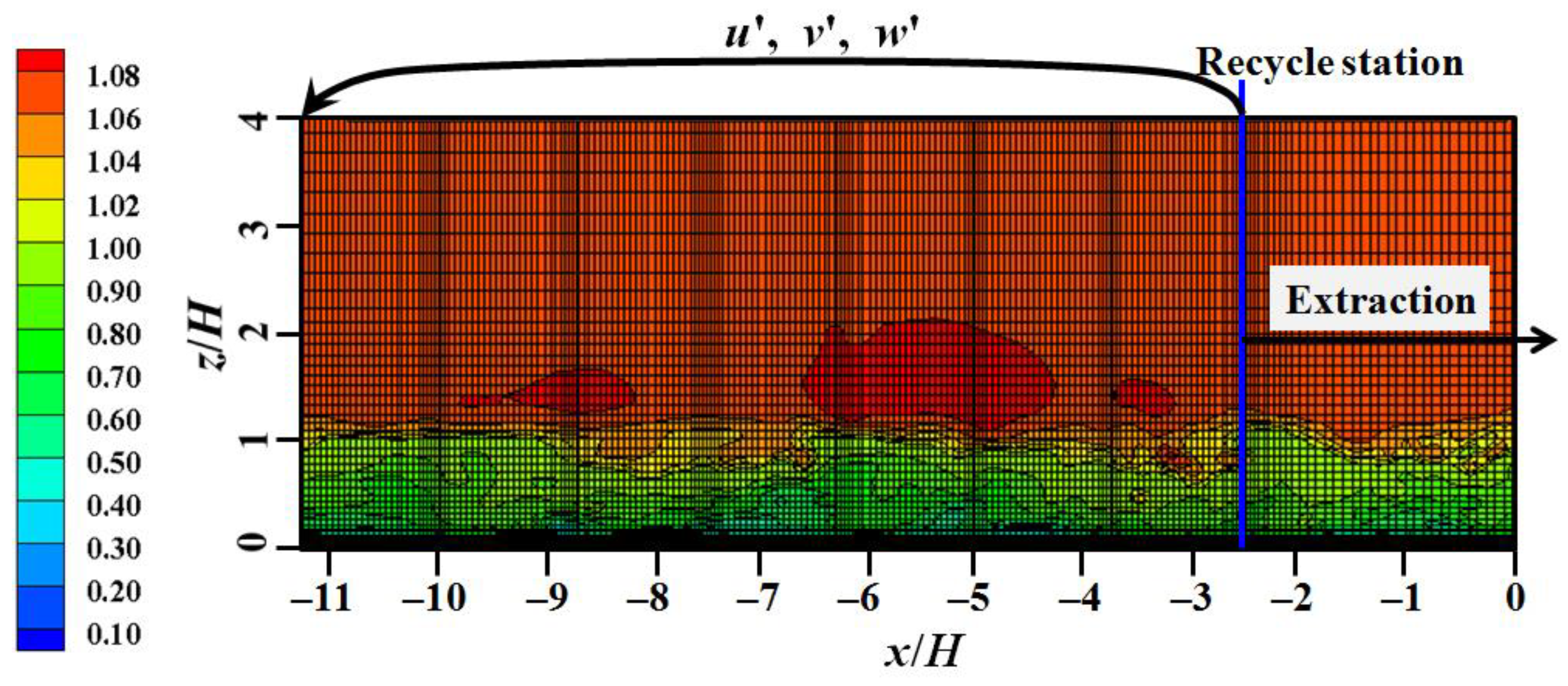
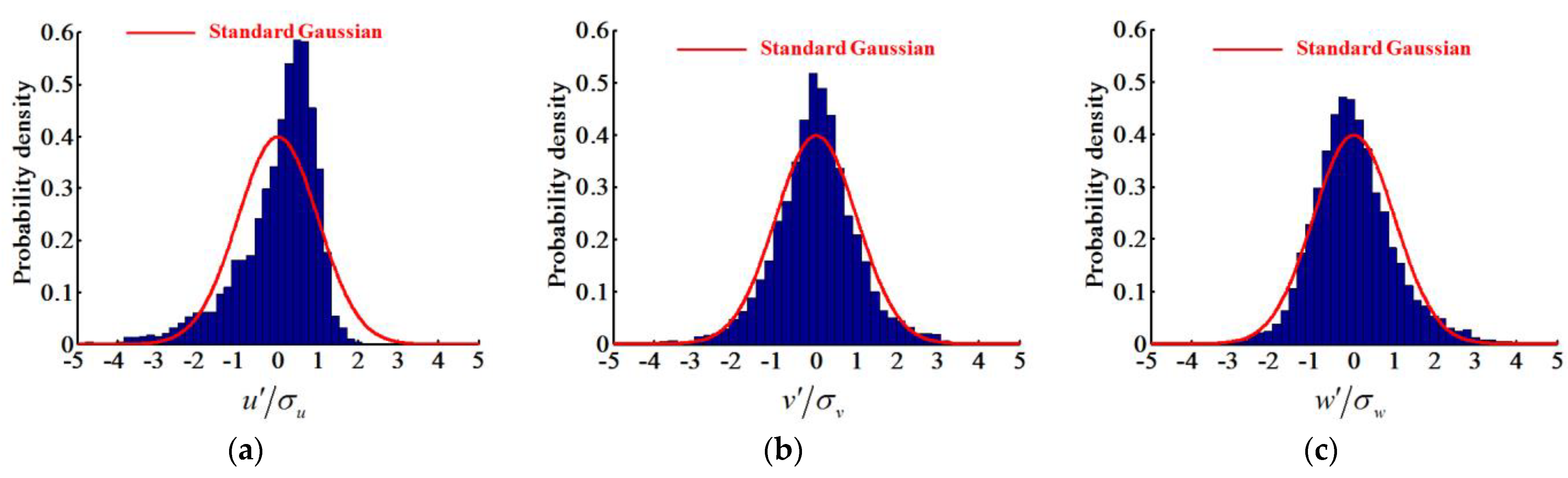
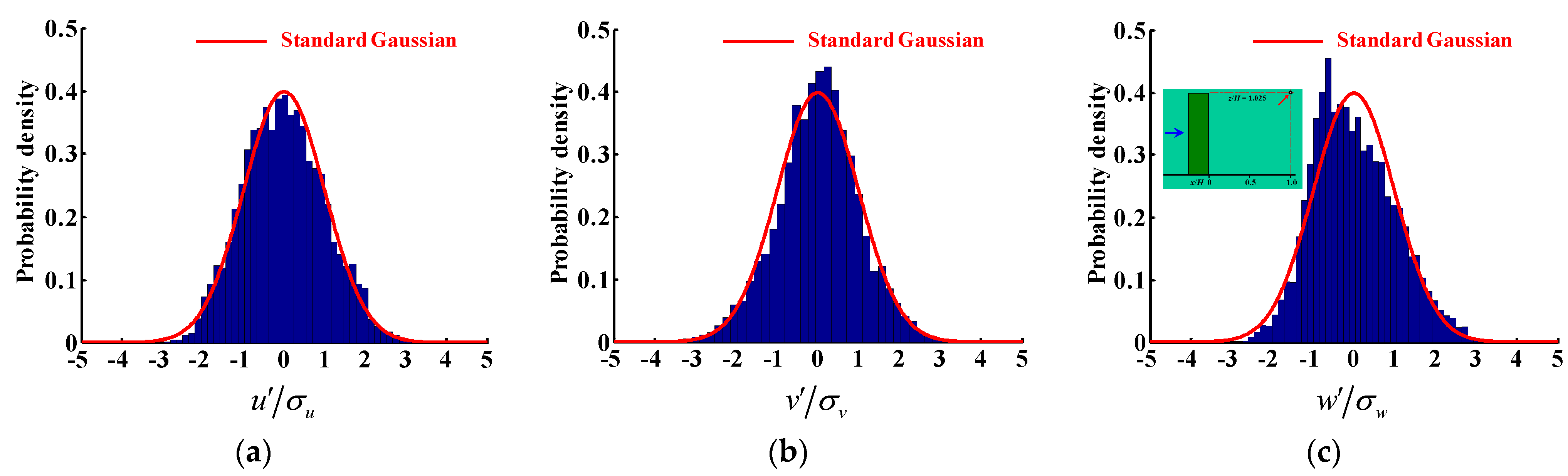
Generating fluctuating inflow data is crucial for achieving an accurate LES for wind engineering applications [2,20]. In this study, turbulent inflow data for LES were generated using Kataoka’s method [3]. The entire simulation domain comprised two regions: a driver region for generating fluctuating inflow data, and a main region to simulate flow and gas dispersion around a high-rise building placed within a turbulent boundary layer. In the driver region, the velocity fluctuations in a downstream station near the outlet were recycled and then assigned to the inlet station at each time step. Figure 1 displays the recycling procedure and the instantaneous distribution of the normalized streamwise velocity (u/UH) when the flow is fully developed, where H (160 mm) is the building height and UH (1.37 m/s) is the mean streamwise velocity in the building-height position. Based on the similarity of the turbulence length scale, the simulated boundary layer corresponded to a geometrical scale of approximately 1:600. Figure 2 presents the probability density functions (PDFs) of the velocity fluctuations at height H for the recycling station. The red solid line indicates the standard Gaussian distribution. All three components of the velocity fluctuations were distributed consistently with the standard Gaussian distribution; however, slightly non-Gaussian features were observed for the streamwise velocity fluctuation. These results are consistent with the Gaussian distributions of the oncoming flow reported by Hu et al. [28] in their simulations of atmospheric boundary layer flow. The extracted instantaneous velocities at each time step at the recycling station were stored and given as the inflow condition for the subsequent main simulations.
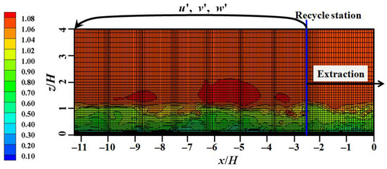
Figure 1.
Inflow turbulence generation for LES (u/UH, the flow field below 4H is displayed).
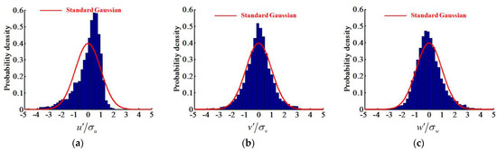
Figure 2.
PDFs of the velocity fluctuations at height H. (a) Streamwise velocity; (b) spanwise velocity; (c) vertical velocity.
3. Simulation Settings
3.1. Simulation Cases and Mesh Systems
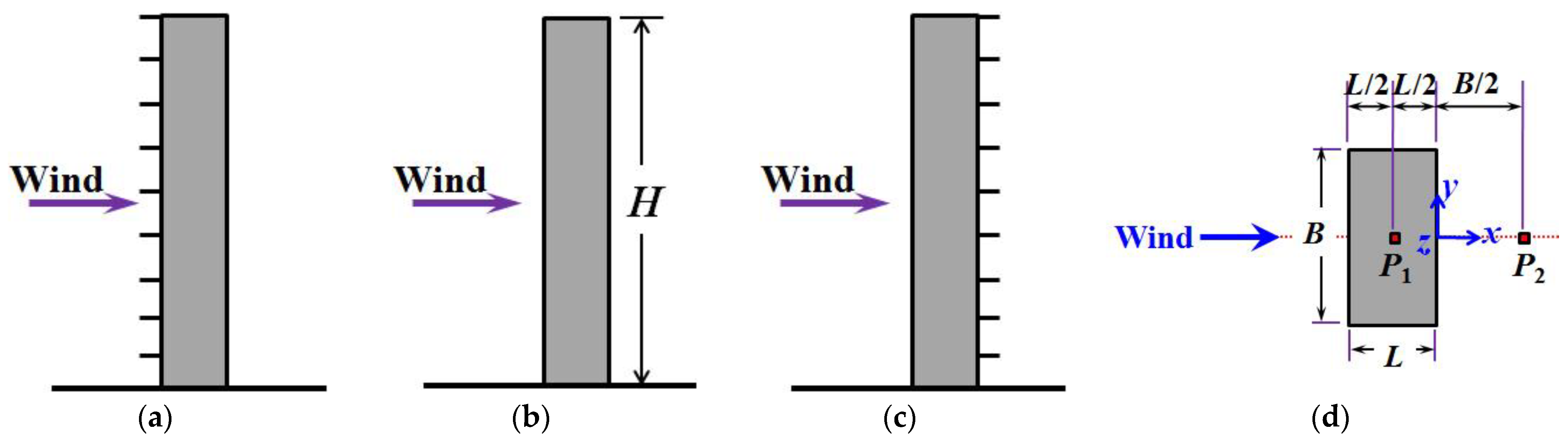
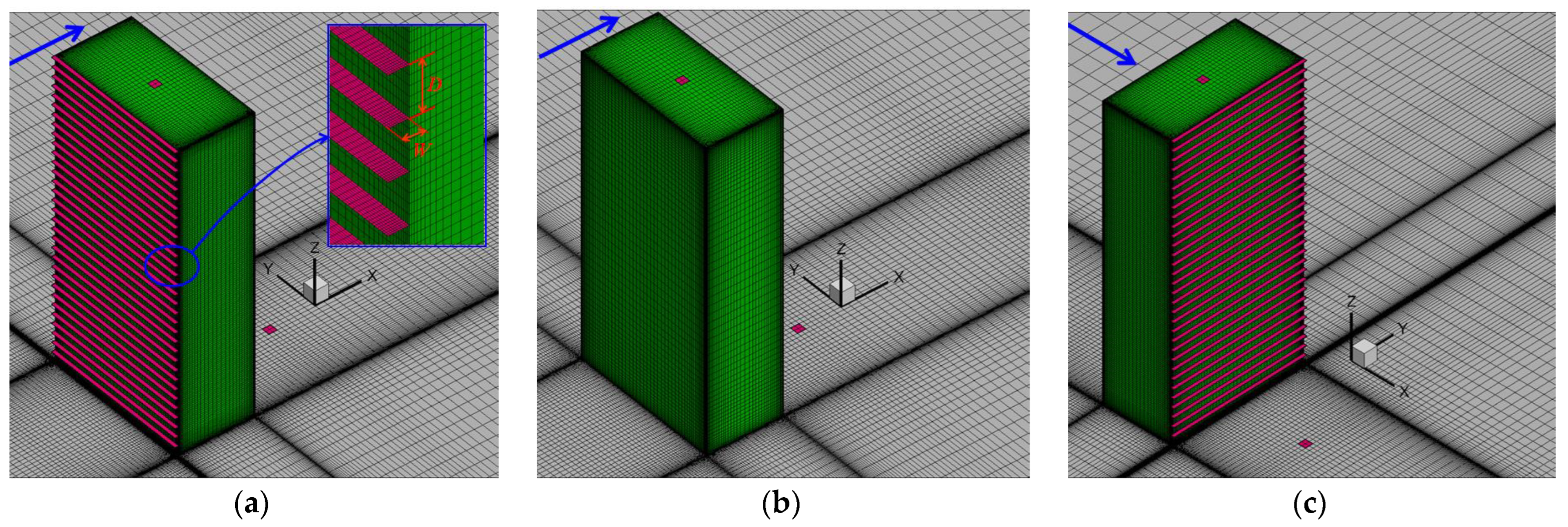
Figure 3a–c presents a schematic view of the building geometry and envelope features. Figure 4 displays the mesh systems used in this study. The studied building was a high-rise with a length (L):width (B):height (H) ratio of 1:2:4. This is the most common shape for commercial or residential high-rise buildings in East Asia. LES was performed for three cases: the base case without facade appurtenances, the case with windward overhangs, and the case with leeward overhangs. The mean velocity profile of the oncoming flow followed a logarithmic law. The building height H was 160 mm, and UH = 1.37 m/s was the mean streamwise velocity at the top of the building. The Reynolds number, based on UH and the building width B, was approximately 7500. As described previously, the geometrical scale of the generated atmospheric boundary layer was approximately 1:600. Accordingly, the building was divided into 32 floors in the vertical direction and a total of 32 overhangs were set on the windward or leeward surface of the building in the cases with appurtenances. Hence, the distance between overhangs was D = 5 mm in the vertical direction, corresponding to a height of 3 m per floor at the full scale. The width of the overhangs was W = 2 mm, corresponding to 1.2 m for the full-scale case.
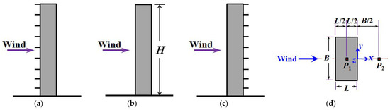
Figure 3.
Building geometry and envelope features. (a) Windward overhangs; (b) base case without overhangs; (c) leeward overhangs; (d) positions of the two gas discharge holes (red).
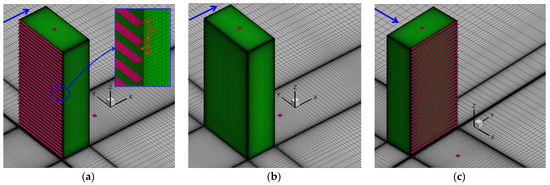
Figure 4.
Mesh systems. (a) Windward overhangs; (b) base case without overhangs; (c) leeward overhangs.
The pollutant investigated in this study was ethylene (C2H4). A tracer gas with an ethylene concentration of 5% was released from two small square holes with an area of 19.36 mm2, one at the center of the rooftop and another on the floor behind the building (0.25H from the leeward wall), as shown in Figure 3d. The discharged mixed gas flow rate was q = 9.17 × 10⁻⁶ m3/s, and the reference concentration was C0 = 5% × q/(UHH2). The emitted gases from the rooftop and ground were denoted as pollutants P1 and P2, respectively. Simultaneously studying gas dispersion from different source locations can improve our understanding of the influence of wind flow on gas dispersion behaviors.
Rectangular meshes were used for all of the simulations; these are summarized in Table 1. The depth of the first fluid cells on the wall surfaces was set to 0.2 mm to ensure that the nondimensional wall distance y+ was less than 1.0; this is required for LES. The grid increase ratio was controlled to be less than 1.20 for most of the edges. In addition, 50, 65, and 80 grids were used to split the edges for the building of the base case in the x, y, and z directions, respectively. The gas discharge holes were square (4.4 × 4.4 mm2), and 2 × 2 = 4 elements were used for their discretizations. For the base case without overhangs, a total cell number of 5.8 million was used to accurately capture the characteristics of the turbulence and pollutant statistics around the building. This mesh was much finer than that used in previous studies [21,29] for the simulation of wind flow around a high-rise building with a square cross-section and a similar Reynolds number. For the simulation cases with overhangs, both coarse and fine mesh systems with 4.2 million and 9 million cells, respectively, were generated to determine the mesh sensitivity. For the coarse-mesh system, the number of grids between overhangs (D) and along overhangs (W) were 3 and 6, respectively; the corresponding values for the fine-mesh system were 5 and 10.

Table 1.
The mesh systems.
3.2. Numerical Procedures and Boundary Conditions
In this study, the open-source software OpenFOAM (version 5.0) was used to simulate the wind flow and gas dispersion phenomena. The governing equations for LES are the continuity, momentum, and gas transport:
where the superbar “―” represents the filtered variables; c is the volume percentage; j = 1, 2, 3 indicates the three spatial coordinates; ν is the kinematic viscosity; νSGS is the sub-grid scale (SGS) viscosity; Sc is the Schmidt number; and σt is the SGS turbulent Schmidt number. Because only the SGS eddies are modeled in an LES, their influence on the model is small. Therefore, the commonly used value of 0.7 was selected for both Sc and σt.
The standard Smagorinsky model [30] was selected as the SGS model for LES, and νSGS was calculated as follows:
where CS is the model constant. A model constant of CS = 0.12 was adopted in this study, and a van Driest damping function [31] was used to account for the near-wall effect in the region where y+ is less than 500. ∆ is the filter truncation scale. is the large-scale strain rate tensor and is calculated as follows:
The size of the computational domain was 7.5H in the spanwise direction and 6.25H in the vertical direction. The length of the domain was 12.5H in the streamwise direction (2.5H ahead of the leeward surface, 10H behind the building). No-slip boundary conditions were applied for all wall surfaces. A vertical velocity of 0.474 m/s was set for both of the gas discharge holes. The generated fluctuating inflow data from the pre-simulation were used as the inflow boundary conditions. For the concentration fields, a value of zero was assigned to the inflow boundary of the domain, and 5% was set for the boundary of each gas discharge hole. The physical time step Δt was set to 10−4 s to make the largest Courant number less than 1 to ensure that the simulation was stable. Symmetry conditions (the normal gradients of all the flow variables are zero) were used for the two lateral and top boundaries of the domain. A zero-gradient condition was used for the outlet boundary.
An implicit second-order backward differencing scheme was adopted for temporal advancement. A second-order central differencing scheme was used for the convection terms of the momentum equation. The pressure implicit with the operator splitting algorithm was used for the pressure–velocity calculations, and 140 units of nondimensional time t* (t* = t × UH/H) were first allowed to enable the flow to develop. Time averaging began after the flow field had fully developed, and 160 units of nondimensional time were used for time averaging to ensure that the mean data was reliable.
4. Results and Discussion
The length of the averaging time is a key factor for determining the mean flow variables in an LES. Although a long simulation time can ensure that the averaged values are reliable, the simulation time is limited in practical engineering applications. Therefore, researchers must strike a favorable balance between simulation time and the reliability of the averaged results for LES. This section discusses the influence of the averaging time on the mean results and investigates the turbulence and pollutant statistics around the building for the base case without overhangs. The effects of windward and leeward overhangs on local wind flow and pollutant statistics were investigated in the other cases.
4.1. Validation of the LES Model
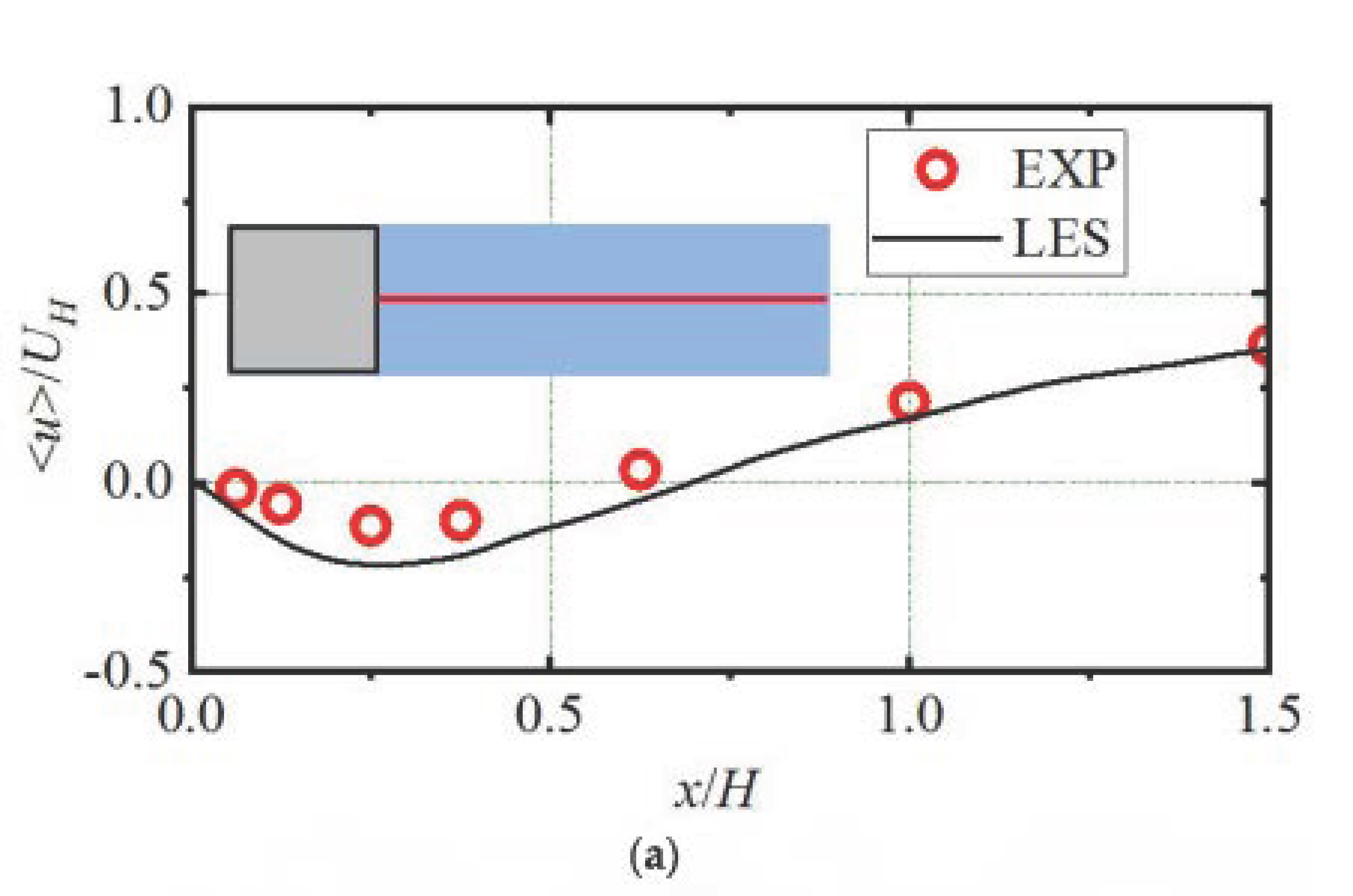
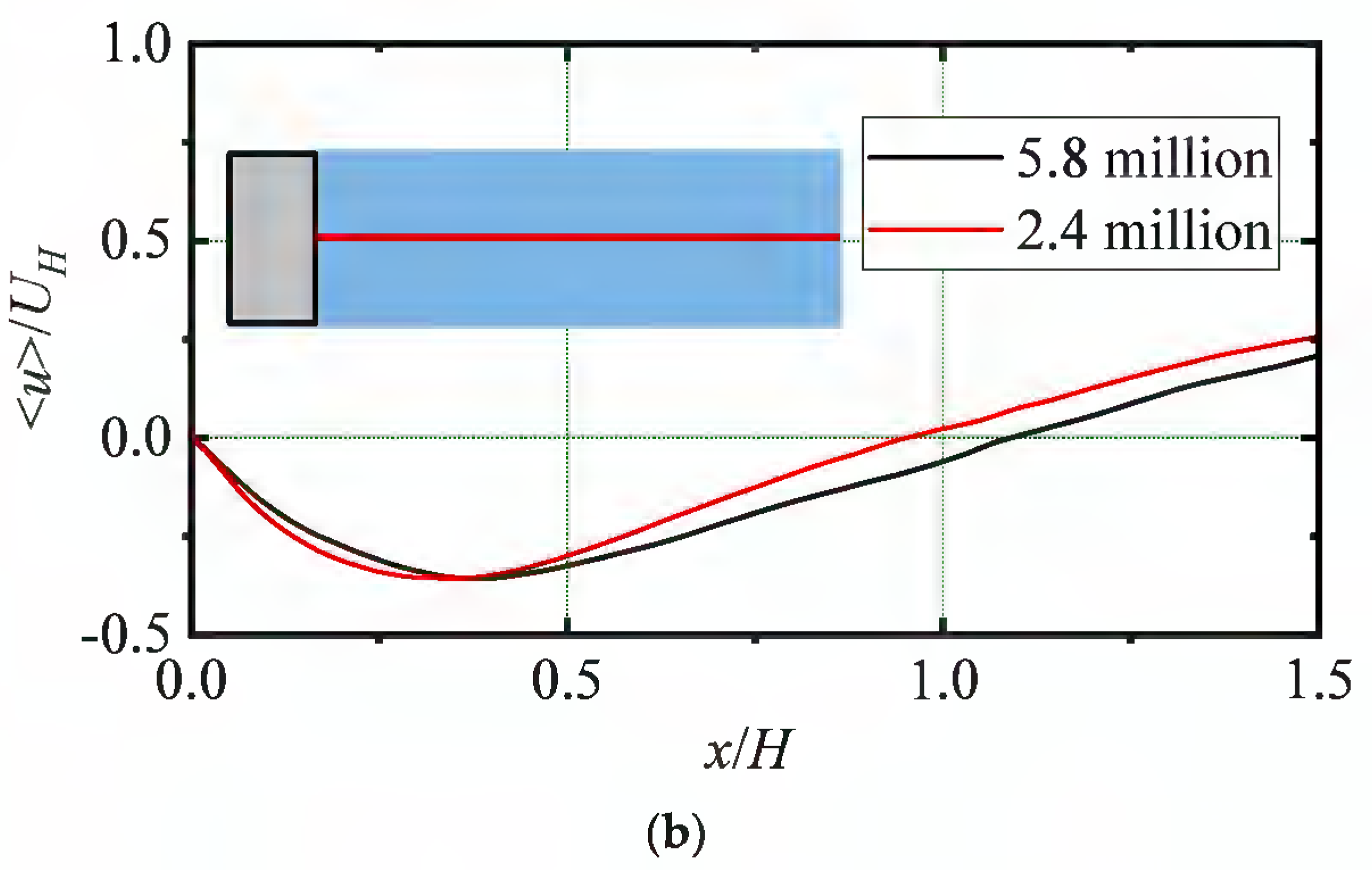
Before the simulations, the numerical algorithm and parameter settings for LES used in this study were validated against wind tunnel experiments on wind flow around a high-rise building with a square cross-section [21]. Figure 5a presents the comparisons of mean streamwise velocity along a horizontal line in streamwise direction (x/H is from 0 to 1.5, y/H = 0, z/H = 0.25). The calculated mean streamwise velocity by LES shows a favorable agreement with the experiment. The LES model used in this study was also validated by comparisons with the wind tunnel experiment in a thermal environment in previous studies [20,32].


Figure 5.
Distributions of mean streamwise velocity along a horizontal line in a streamwise direction (y/H = 0, z/H = 0.25). (a) Validation of the LES model; (b) grid sensitivity check for the base case.
Figure 5b compares the mean streamwise velocities obtained using a fine-mesh system (5.8 million) and a coarse-mesh system (2.4 million) along a horizontal line for the base case. The mesh density only slightly affects the results.
4.2. Influence of the Averaging Time
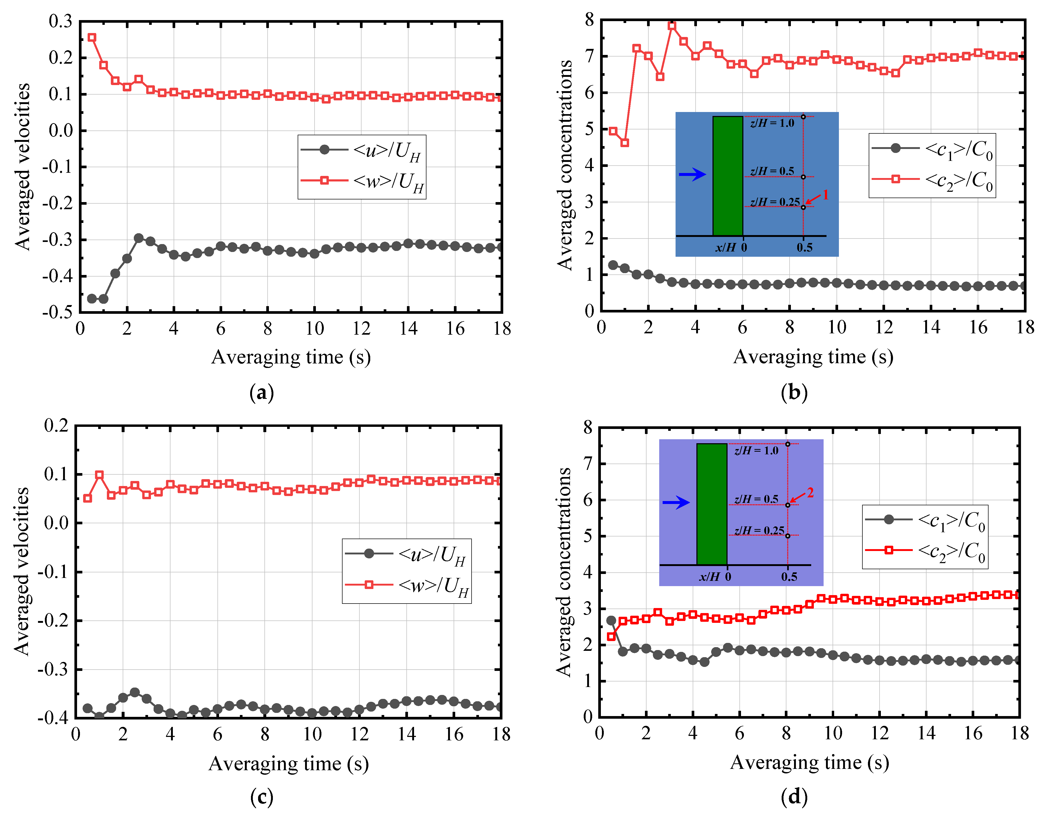
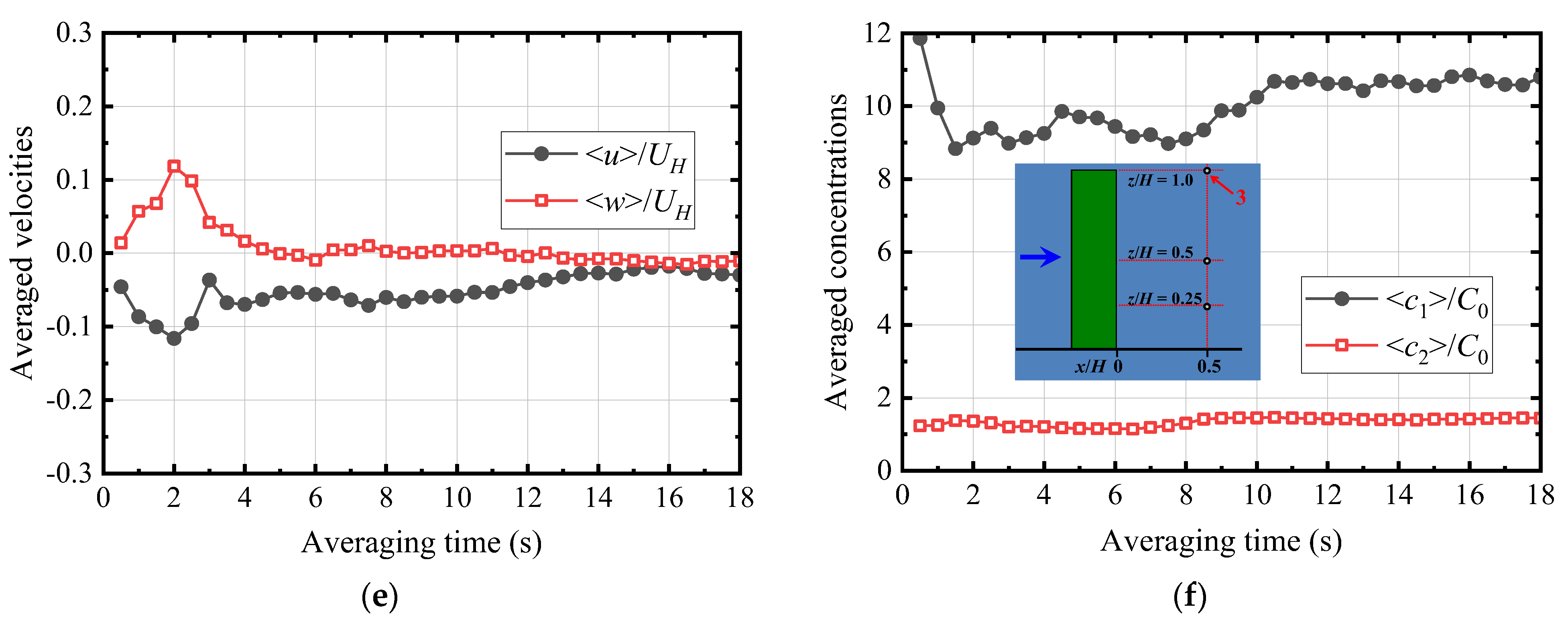
Figure 6 displays the time series of the spanwise velocity fluctuation behind the building at the positions x/H = 0.125 and z/H = 0.5. The flow around an isolated high-rise building is dominated by the flow separation and large-scale periodic vortex motion. In this study, the data for all flow variables were averaged over 160 nondimensional time units t*, which corresponded to more than 30 periodic vortex-shedding cycles. This can be approximately identified from the number of peaks of the wave shown in Figure 6. Figure 7 presents the changes in the average velocities and concentrations over the averaging time at three representative points in a vertical line behind the building (along x/H = 0.5, y/H = 0). The three points are located at low (z/H = 0.25), middle (z/H = 0.5), and high (z/H = 1.0) positions, respectively. The results revealed that the necessary averaging time differed between locations for a given variable. For the mean velocities, the final values were quickly achieved after time averaging for 6 s at point 1 and point 2. However, at point 3, the averaged streamwise velocity was unstable until after 12 s of time averaging; this was attributed to the flow separation and down-washing at this location. For the concentration field, shorter averaging times were required for low-concentration stations; longer averaging times were necessary for high-concentration positions because of the influence of large vortex motions. For the P2 concentration at point 1 and the P1 concentration at point 3, the averaged values become stable after t = 14 s. Hence, the averaging time required for reliability was longer for the concentration fields than for the velocity fields. A possible reason for this difference is discussed in Section 4.4. Therefore, a long averaging time corresponding to at least 20 periodic vortex-shedding cycles was necessary to obtain accurate mean flow variables for flow and gas dispersion around an isolated building for the LES.
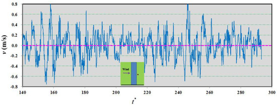
Figure 6.
Time series of spanwise velocity fluctuation behind the building (x/H = 0.125, y/H = 0, z/H = 0.5).
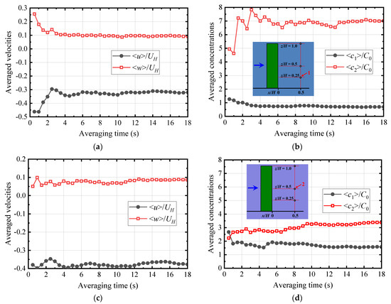

Figure 7.
Changes in averaged values with averaging time at different points. Averaged (a) velocities at point 1; (b) concentrations at point 1; (c) velocities at point 2; (d) concentrations at point 2; (e) velocities at point 3; (f) concentrations at point 3.
4.3. Turbulence Statistics
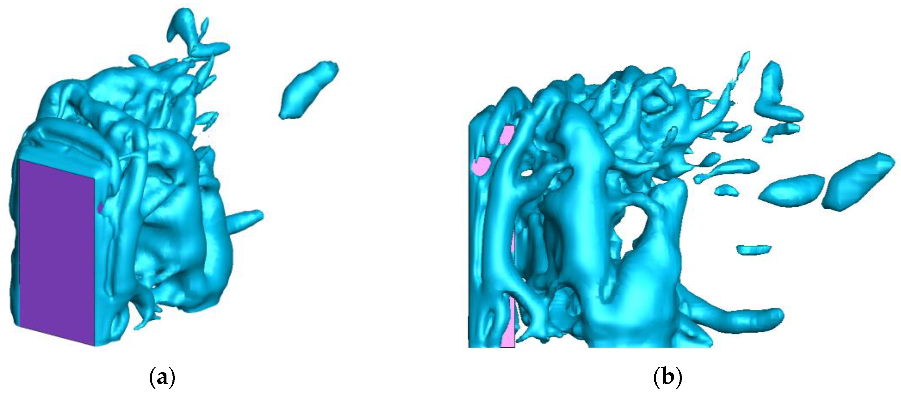
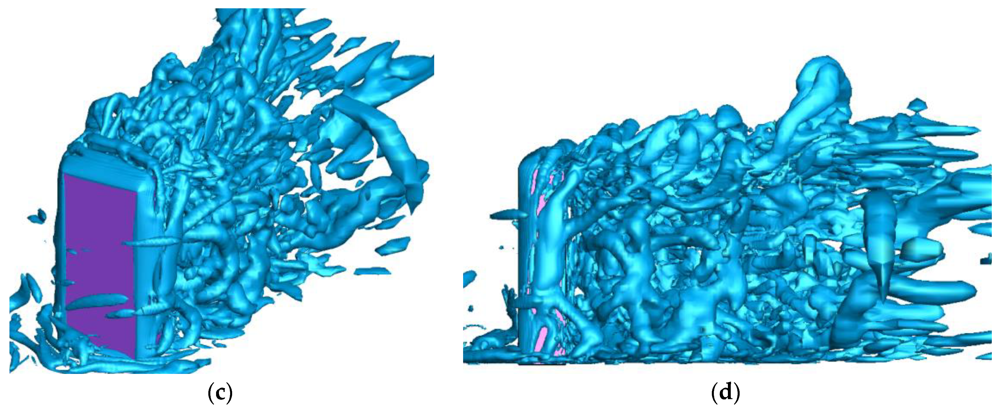
Figure 8 displays the vortex structures around the building as identified by the low-pressure center (p = −0.5 Pa) and the positive second invariant of the velocity gradient [Q = 500 s−2]. The smooth side vortex was generated from the edges of the front surface after flow separation; it then broke down at a downstream station. A series of large disorderly vortices were formed in the wake region behind the building. Overall, the vortex shapes identified from the low-pressure center and Q criteria are similar, indicating that both methods can be used to identify coherent vortex structures. The low-pressure center can be used to identify the vortex structures because the pressure is usually low in the center of a vortex in a turbulent flow. The large vortices identified with the low-pressure center are slightly coarser. Compared with the low-pressure center, the Q criteria can be better used to identify fine vortex structures, such as the horseshoe vortex ahead of the building near the ground. Hence, the Q criteria is more reliable for identifying the coherent vortex structures of flow around a blunt body.

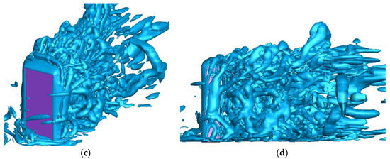
Figure 8.
Vortex structures. (a) Overall, p = −0.5 Pa; (b) side views, p = −0.5 Pa; (c) overall, Q = 500 s−2; (d) side views, Q = 500 s−2.
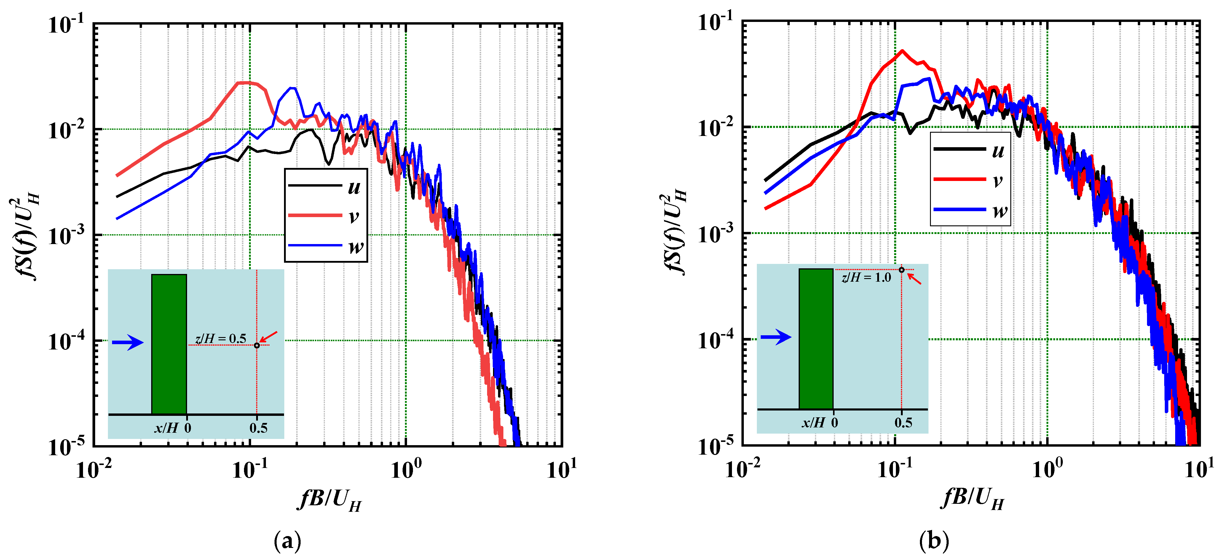
The power spectrum densities (PSDs) of u, v, and w velocity fluctuations at a point behind the building (x/H = 0.5, z/H = 0.5) are presented in Figure 9a. The PSDs of the u and w velocities are smooth, but a clear peak value is observed in the PSD of the v velocity fluctuations at a nondimensional frequency of approximately 0.1. From the relation fB/UH = 0.1, we can obtain the frequency and period of the periodic vortex-shedding phenomena, suggesting that the total simulation time of this study (18 s) corresponds to approximately 32 periodic vortex-shedding cycles. This is consistent with the number of peaks in the wave in Figure 6. The PSDs of all velocity components decrease sharply near fB/UH = 5, indicating that the mesh system was insufficiently fine to capture small eddies with high frequencies. Figure 9b displays the PSDs of the velocity fluctuations at point (x/H = 0.5, z/H = 1.0). Although distinct peaks were observed in the PSDs of the v velocity fluctuations, the difference in the magnitude of the power spectrum among three velocity fluctuations was small for the eddies in the energy-containing range with low frequencies, indicating that the flow was dominated by not only the periodic vortex-shedding phenomena but also other flow features, such as flow separation and down-washing.
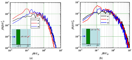
Figure 9.
Power spectrum densities of u, v, and w velocity fluctuations behind the building. (a) At the point (x/H = 0.5, y/H = 0, z/H = 0.5); (b) at the point (x/H = 0.5, y/H = 0, z/H = 1.0).
Figure 10 and Figure 11 present the PDFs of the u, v, and w velocity fluctuations at two points behind the building located inside and outside the recirculation region, respectively. The occurrence position of the maximum frequencies was near zero, and all three components of the velocity fluctuations were in favorable agreement with the standard Gaussian distribution at both points. These distribution patterns are similar to that of the oncoming flow shown in Figure 2. Slight non-Gaussian features are observed in Figure 11c. It is possible that the flow did not reach the statistical stability at this position because of insufficient simulation time. This can be demonstrated by the change in mean velocity with averaging time at another position nearby shown in Figure 7e, in which the averaged vertical velocity <w> still slightly changed even after 18 s’ time averaging.
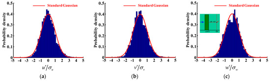
Figure 10.
PDFs of the wind velocities at point (x/H = 0.5, y/H = 0, z/H = 0.5). (a) Streamwise velocity u; (b) spanwise velocity v; (c) vertical velocity w.
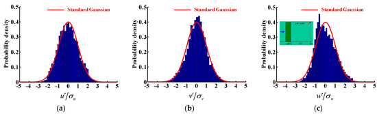
Figure 11.
PDFs of the wind velocities at point (x/H = 1.0, y/H = 0, z/H = 1.025). (a) Streamwise velocity u; (b) spanwise velocity v; (c) vertical velocity w.
4.4. Pollutant Statistics
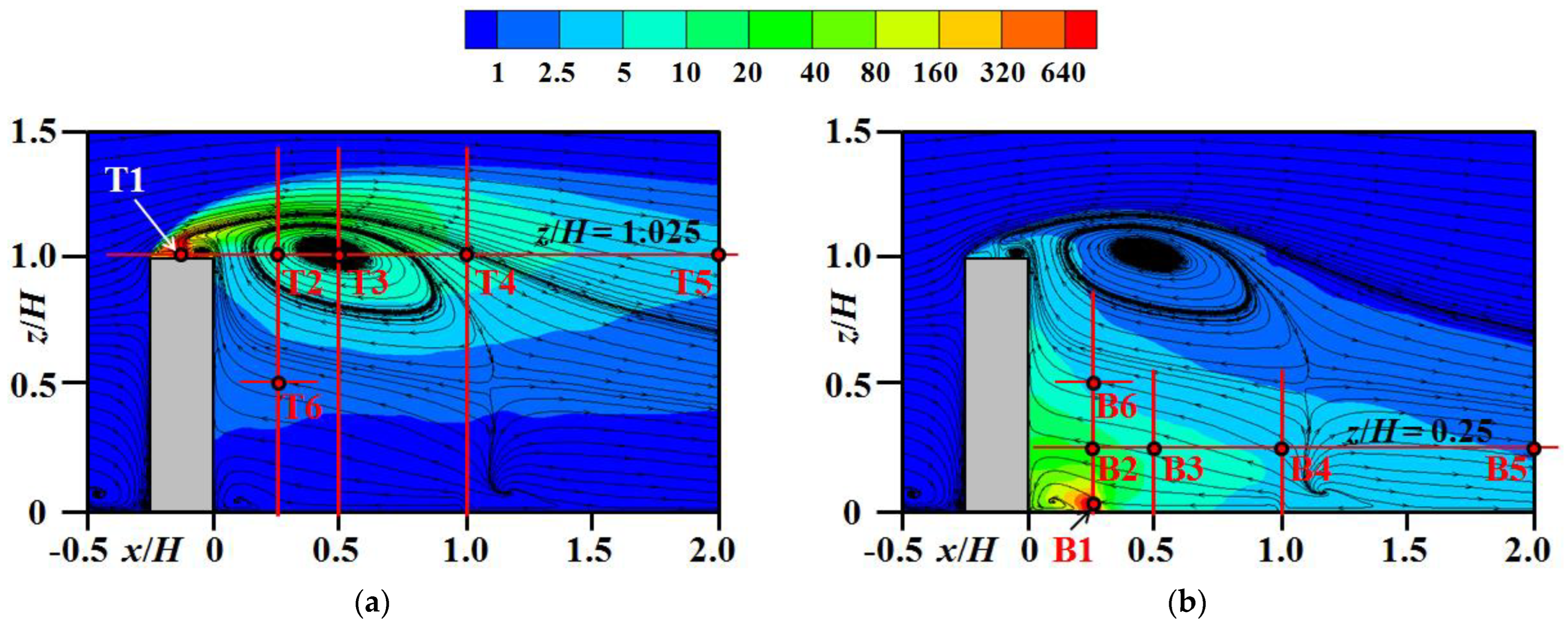
The mean concentration distributions for pollutants discharged from both the rooftop and ground are displayed in Figure 12. The mean streamlines are also shown in the figure. A large recirculation region formed behind the building with its core located near the building-height position. The P1 pollutant discharged from the rooftop was mainly concentrated at the building-height station after it was blown downstream. Although some P1 pollutant was also blown to the wake of the building at a lower height because of the downwash flow and turbulence, the concentration was low near the leeward surface of the building and the ground. Because the source point of the P2 pollutant was located inside the recirculation region, the P2 pollutant was not easily transported out of the recirculation region; most of it accumulated behind the building near the leeward surface. Some P2 pollutant was even transported to higher floors at a high concentration by the upward flow and turbulence. This indicates a higher exposure risk for the people living on higher floors.

Figure 12.
Mean gas distributions and the studied locations for concentration statistics. (a) P1 gas (rooftop dispersion); (b) P2 gas (ground dispersion).
Pollutant statistics analysis from a large number of representative stations is useful for determining the dispersion patterns of a pollutant. Therefore, the pollutant statistics were studied for the points in Figure 12. Points T1 to T5 were located in a horizontal line slightly above the building (z/H = 1.025). Point T1 was just above the source location, and the distance from the source location gradually increased for points T2 to T5. Point T6 was located in a low-concentration region inside the wake behind the building (x/H = 0.25, z/H = 0.5). Point B1 was located just above the source station of the P2 pollutant. Points B2 to B5 were located in a horizontal line in the wake behind the building (z/H = 0.25). Point B6 was located at x/H = 0.25 and z/H = 0.5.
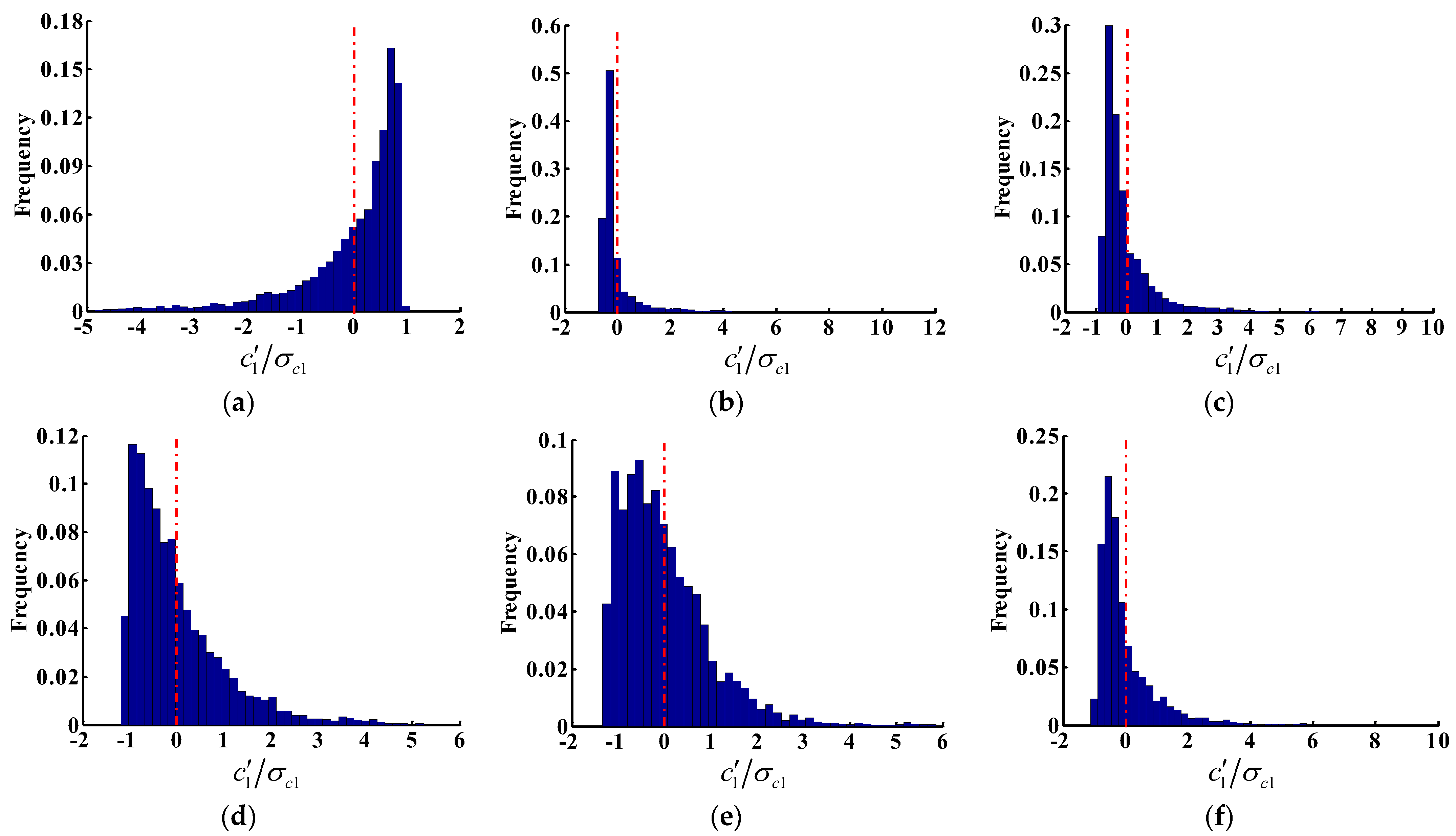
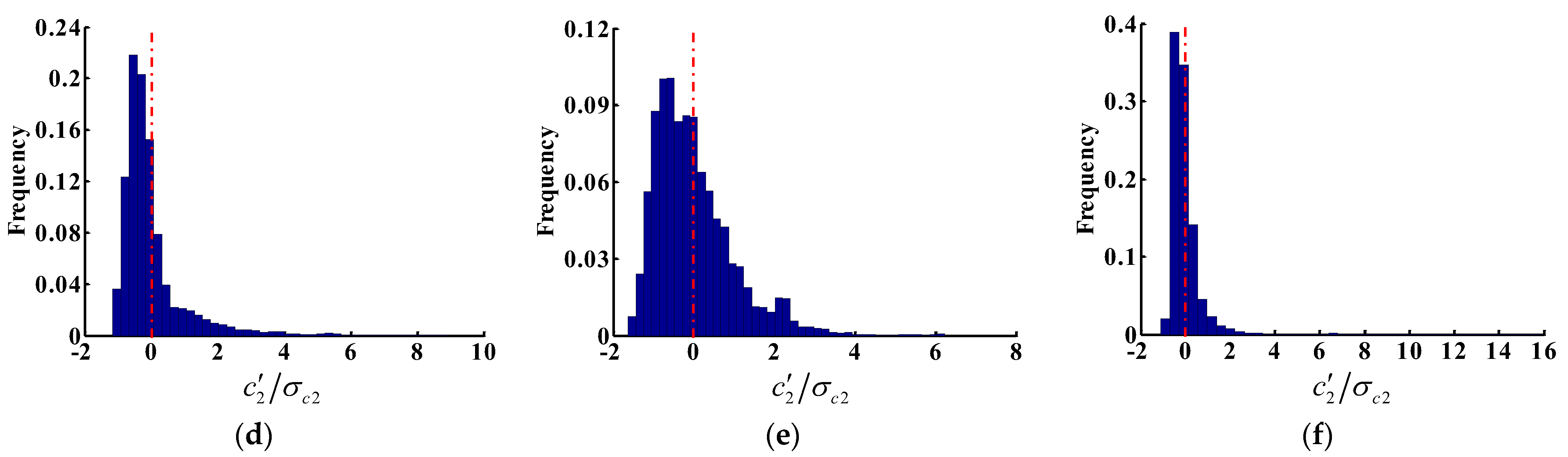
Figure 13 presents the distributions of the occurrence frequency for the P1 concentration fluctuations at points T1 to T6. Similarly, Figure 14 presents the frequency distributions of the P2 concentration fluctuations from point B1 to point B6. Unlike the PDF distributions of the velocity fluctuations shown in Figure 10 and Figure 11, the frequency patterns of pollutants were far from a Gaussian distribution at all of the locations. At locations far away from the source point, negative fluctuations were most frequent, but the maximum positive fluctuations were much larger. This was most notable for the P1 pollutant at point T2 and the P2 pollutant at point B2; for these stations, the maximum frequency was greater than 50% or 70%, respectively, and the maximum positive fluctuations reached nearly 12 to 16 standard deviations. Understanding this characteristic is critical for highly hazardous gases; instantaneous high values can result in a high exposure risk to people even if they are only exposed for a short time. At the locations near the source point, various frequency distribution patterns were observed. For the P1 pollutant at point T1, most instantaneous values were larger than the mean value, but the maximum negative fluctuation was much larger. For the P2 pollutant at point B1, the occurrence frequencies of positive and negative fluctuations were nearly equal, and the difference between the largest and smallest frequencies was small.
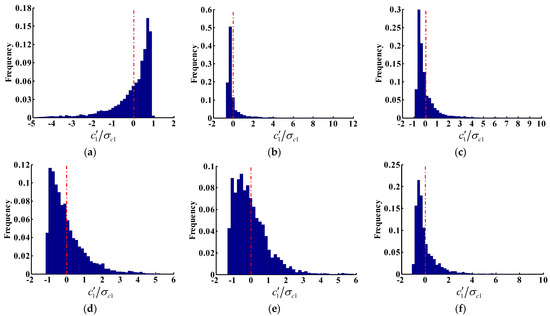
Figure 13.
Frequency distributions of P1 pollutant concentration at (a) station T1; (b) station T2; (c) station T3; (d) station T4; (e) station T5; (f) station T6.
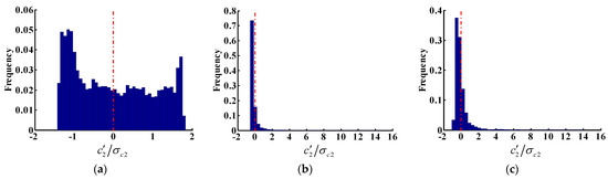
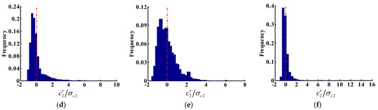
Figure 14.
Frequency distributions of P2 pollutant concentration at (a) station B1; (b) station B2; (c) station B3; (d) station B4; (e) station B5; (f) station B6.
The intermittent occurrence of extremely high or low concentrations is an important characteristic of pollutant dispersion in turbulent flow. In studies conducted by Jiang and Yoshie [21] on gas dispersion around high-rise buildings with different side ratios and by Gousseau et al. [10] for gas dispersion around an isolated cubical building, the first frequency distribution pattern (in Figure 13b–f and Figure 14b–f) was observed at most locations in the flow field. The second distribution pattern found in this study (Figure 13a) occurred only near the source location of the pollutant. The third distribution pattern shown in Figure 14a is seldom observed because the turbulent flow and dispersion around an isolated building are usually dominated by large-scale vortex motion. Compared with that for a velocity field, the necessary averaging time should be longer for a concentration field because of its asymmetric or non-Gaussian frequency distributions.
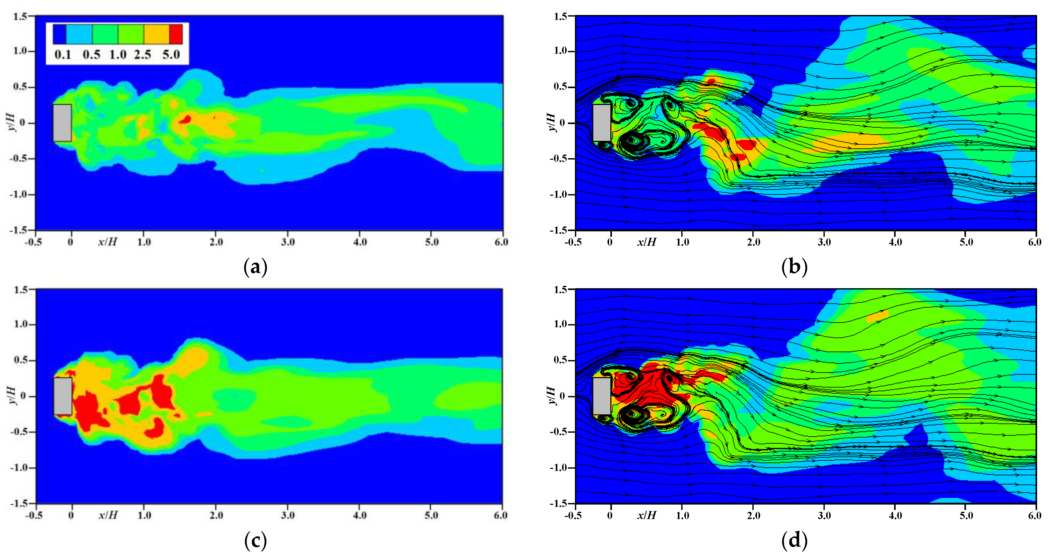
Figure 15 displays the normalized instantaneous P1 and P2 concentration distributions at two different representative instants on a horizontal plane (z/H = 0.5). The instantaneous distributions of streamlines are also displayed in Figure 15b,d, in which some eddies were generated near the side surface after flow separation and some large eddies had already moved downstream. After the P1 pollutant was transported to the wake behind the building from a high position, the dispersion patterns of P1 and P2 pollutants were quite similar; they were both affected by the large-scale periodic vortex-shedding phenomena. When the large-scale vortex motion was weak at time t1, the contour lines were smooth at the downstream stations for both P1 and P2 pollutants. At another instant, t2, when the periodic vortex-shedding phenomena was strong, the instantaneous distributions of both the P1 and P2 pollutants had a distinct meandering pattern.
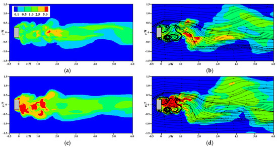
Figure 15.
Instantaneous P1 and P2 concentration distributions c/C0 at different instants in a horizontal plane (z/H = 0.5). (a) P1 concentration at time t1; (b) P1 concentration at time t2; (c) P2 concentration at time t1; (d) P2 concentration at time t2.
4.5. Effects of Overhangs
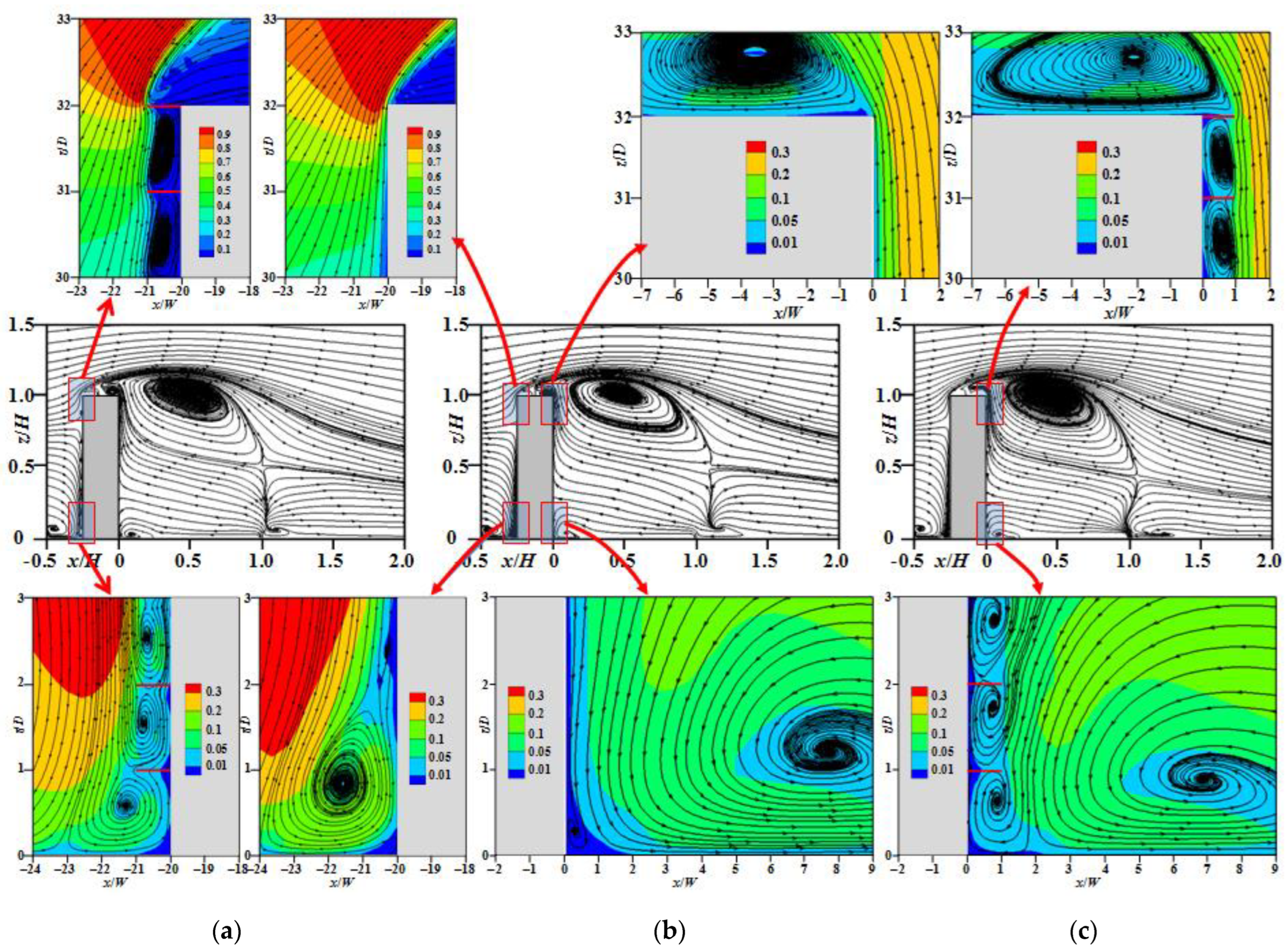
Figure 16 presents comparisons of the overall wind flow and local flow structures near the building facade for the three cases. A fine mesh system was used to simulate the cases with overhangs set on both the windward and leeward surfaces. Overall, the differences in the overall flow field among the three cases were small; however, the local wind flows near the building facade were greatly affected by the overhangs. For the case with windward overhangs, the ascending air in front of the building impinged on the overhangs and then formed a clockwise recirculation inside the upper floors; the descending air formed a counterclockwise recirculation inside the lower floors after it struck the overhangs. The opposite was observed for the case with leeward overhangs; counterclockwise recirculation occurred for most of the upper floors, whereas clockwise recirculation occurred for the lower floors near the ground. A small counterclockwise recirculation formed in front of the building near the ground in the base case; its size was reduced by the windward overhangs. The leeward overhangs also changed the counterclockwise recirculation near the back corner above the rooftop in the base case to a flat recirculation.

Figure 16.
Influence of overhangs on mean wind flow. (a) Windward overhangs; (b) base case without overhangs; (c) leeward overhangs (the contours in the figure represent the nondimensional velocity magnitude Umag/UH).
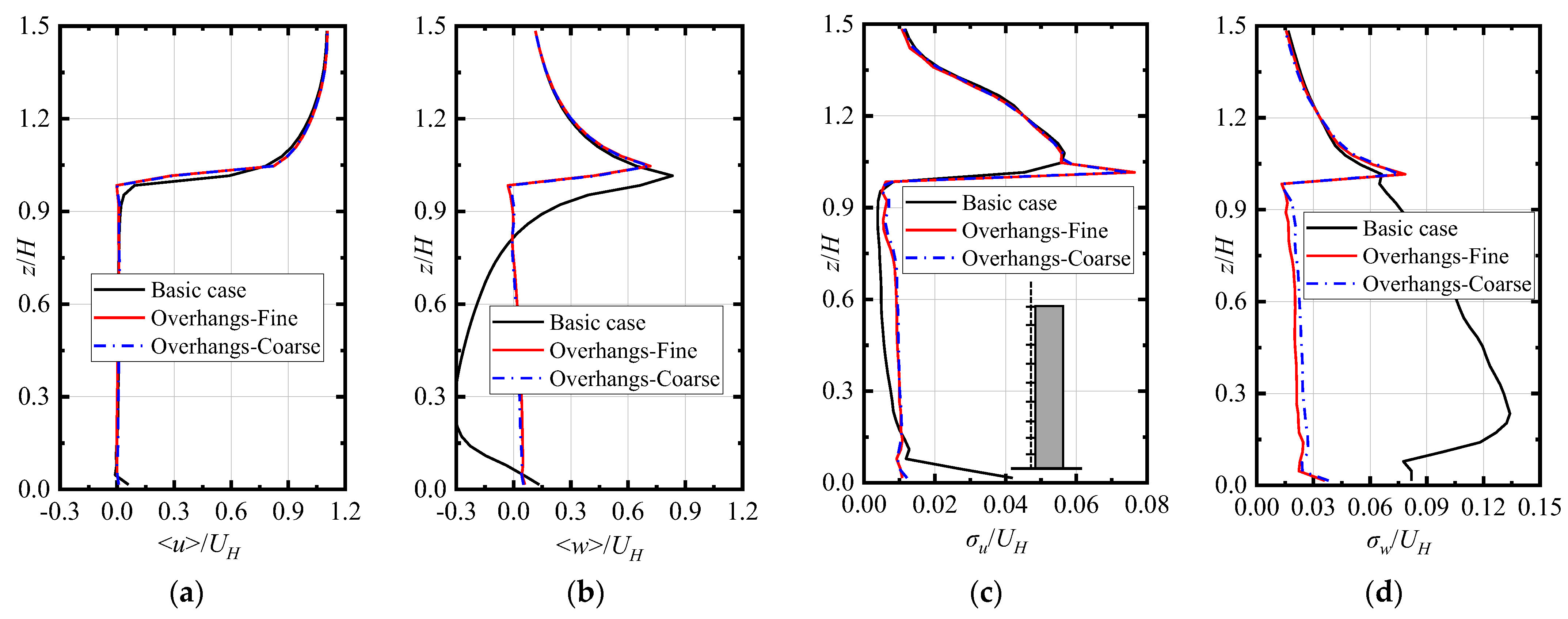
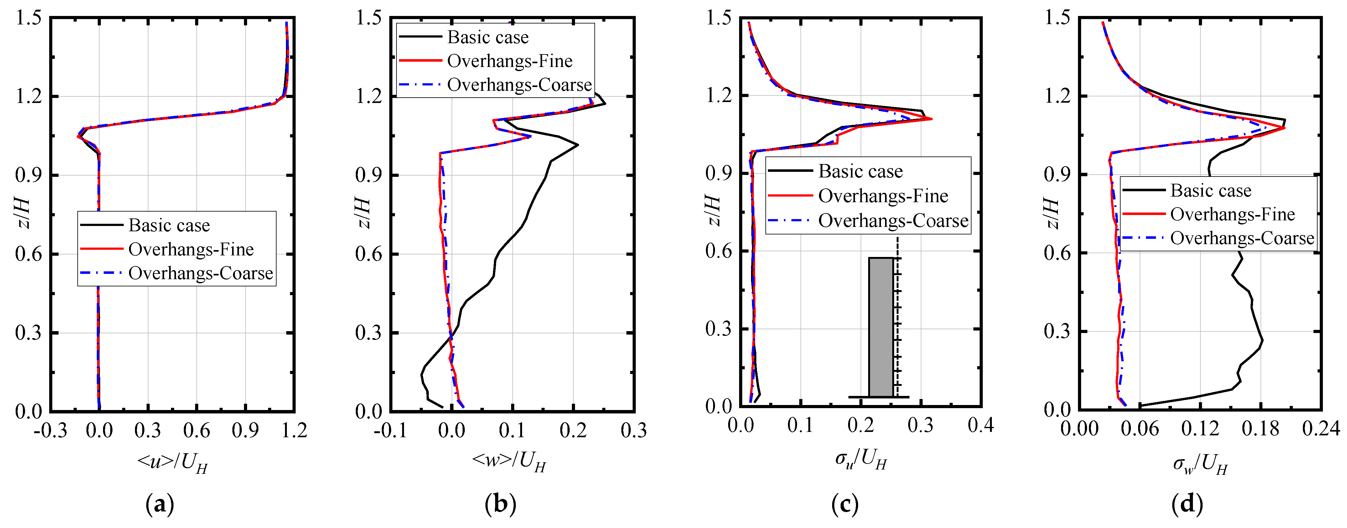
Figure 17 and Figure 18 present comparisons of the mean velocities and their fluctuations along a vertical line through the middle of overhangs for the windward and leeward overhang cases, respectively. For the cases with overhangs, the results for coarse-mesh simulations are also displayed. The results indicate that the LES was not sensitive to the mesh density for either the windward or the leeward overhang case. Compared with the base case, only the flow near the building facades was affected by the overhangs. The differences in mean streamwise velocity and its fluctuations between the base case and the cases with overhangs were small. The existence of overhangs mainly affected the vertical velocity and its fluctuations near the building facade. The mean vertical velocity was greatly reduced and its fluctuations were restricted in the region between overhangs. This strongly affected the pollutant statistics near the overhangs.
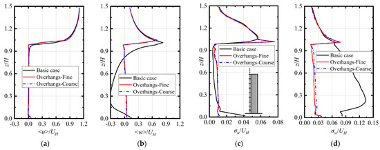
Figure 17.
Distributions of mean velocities and their fluctuations along a vertical line through the windward overhangs. (a) Mean streamwise velocity; (b) mean vertical velocity; (c) standard deviation of streamwise velocity; (d) standard deviation of vertical velocity.
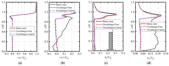
Figure 18.
Distributions of mean velocities and their fluctuations along a vertical line through the leeward overhangs. (a) Mean streamwise velocity; (b) mean vertical velocity; (c) standard deviation of streamwise velocity; (d) standard deviation of vertical velocity.
Figure 19a presents a comparison of the maximum concentration fluctuation for each floor for the base case and that with leeward overhangs. For these positions located between the overhangs, the frequency distributions all had the second pattern shown in Figure 13b–f and Figure 14b–f. The maximum positive fluctuation reached more than eight standard deviations inside most of the floors for the P2 pollutant. At all floors except for some, the maximum concentration fluctuations of both P1 and P2 pollutants were substantially lower for the overhang case than for the base case. This is mainly because of the restriction of vertical velocity fluctuations by the overhangs, as shown in Figure 18d. Figure 19b displays the maximum occurrence frequency for each floor. For the P1 pollutant discharged from the rooftop, the maximum occurrence frequency is high for the floors near rooftop. For the P2 pollutant discharged from the ground behind the building, the maximum occurrence frequency was observed on the sixteenth floor. The leeward overhangs seemed to greatly decrease the maximum occurrence frequency.
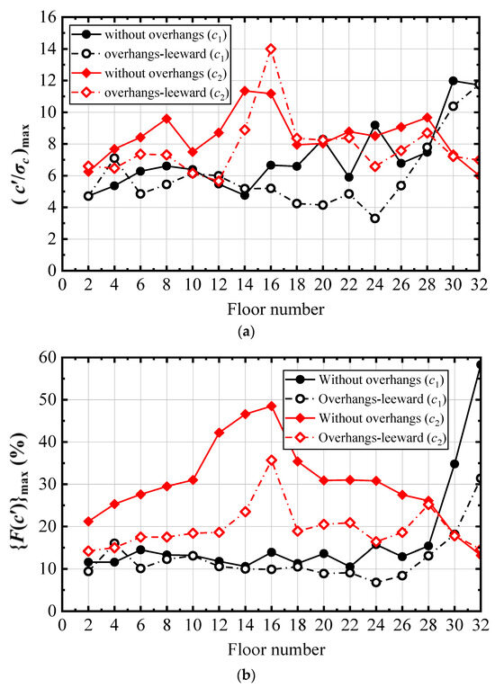
Figure 19.
Pollutant statistics for each floor with and without leeward overhangs. (a) Maximum concentration fluctuation; (b) maximum occurrence frequency.
5. Conclusions
LESs were performed to study the turbulence and pollutant statistics around a high-rise building with a 1:2:4 shape placed within a turbulent boundary layer. The dispersion characteristics of two pollutants discharged from the rooftop and ground behind the building were studied simultaneously. The effects of the averaging time on the LES results were discussed, and the effects of overhangs on the local wind flow and pollutant statistics were summarized.
The necessary averaging time for reliable mean results can differ for the velocity and concentration fields. The mean velocities quickly achieved their final values after only several sections of time averaging for most of the locations. A much longer averaging time was necessary for the concentration field, especially for positions with high concentration and where large vortex motions occurred. The results suggested that a sufficient averaging time of at least 20 periodic vortex-shedding cycles is necessary for LES when simulating flow and gas dispersion around an isolated building.
Complex vortex structures were identified around the building by the methods of the low-pressure center and Q criteria. Large-scale periodic vortex-shedding phenomena were detected from the PSD of spanwise velocity fluctuations and the meandering distribution patterns of the pollutants behind the building.
For both the oncoming flow and the flow around the building, the PDFs of all three velocity components were in favorable agreement with a standard Gaussian distribution. The frequency distribution of the concentration was far from a Gaussian distribution at all locations, and three frequency distribution patterns were observed. For the majority of areas far from the source location, negative fluctuations were most common, but the maximum positive fluctuation was much larger than the maximum negative fluctuations. Near the source point, positive fluctuations occurred more frequently; the occurrence frequencies of positive and negative fluctuations were equal occasionally.
The existence of the overhangs strongly affected the local wind flow near the building facade. Clockwise and counterclockwise recirculation was observed at the upper and lower floors, respectively, for the windward overhangs; the opposite was observed for the case of leeward overhangs. The vertical velocity and its fluctuations were greatly restricted near the overhangs. Both the maximum concentration fluctuation and the maximum occurrence frequency were greatly decreased in the case of leeward overhangs.
Author Contributions
Conceptualization, G.J. and M.W.; methodology, G.J. and T.H.; writing—original draft preparation, G.J.; writing—review and editing, M.W. and T.H.; supervision, G.J.; funding acquisition, G.J. All authors have read and agreed to the published version of the manuscript.
Funding
This research was funded by the National Natural Science Foundation of China (No. 42175102) and by Guangdong Basic and Applied Basic Research Foundation, China (No. 2021A1515010753).
Institutional Review Board Statement
Not applicable.
Informed Consent Statement
Not applicable.
Data Availability Statement
The data presented in this study are available on reasonable request from the first author. The data are not publicly available due to their file sizes and operating system requirements.
Conflicts of Interest
The authors declare no conflict of interest.
Nomenclature
| f | instantaneous value of a quantity |
| <f> | time-averaged value |
| f′ | fluctuation from time-averaged value |
| σf | standard deviation of f |
| x, y, z | three components of space coordinates (m) |
| u, v, w | three components of velocity vector (m/s) |
| p | instantaneous pressure (Pa) |
| c | pollutant concentration (volume percentage) |
| Q | positive second invariant of the velocity gradient (s−2) |
| H | building height (160 mm) |
| B | building width (80 mm) |
| UH | inflow mean velocity at building height (1.37 m/s) |
| q | pollutant emission rate (m3/s) |
| C0 | reference concentration (=q/(UHH2)) |
| νSGS | sub-grid scale viscosity |
| σt | sub-grid scale Schmidt number |
References
- Nozawa, K.; Tamura, T. Large eddy simulation of the flow around a low-rise building immersed in a rough-wall turbulent boundary layer. J. Wind Eng. Ind. Aerodyn. 2002, 90, 1151–1162. [Google Scholar] [CrossRef]
- Tominaga, Y.; Mochida, A.; Murakami, S.; Sawaki, S. Comparison of various revised k-ε models and LES applied to flow around a high-rise building model with 1:1:2 shape placed within the surface boundary layer. J. Wind Eng. Ind. Aerodyn. 2008, 96, 389–411. [Google Scholar] [CrossRef]
- Kataoka, H. Numerical simulations of a wind-induced vibrating square cylinder within turbulent boundary layer. J. Wind Eng. Ind. Aerodyn. 2008, 96, 1985–1997. [Google Scholar] [CrossRef]
- Saeedi, M.; LePoudre, P.; Wang, B. Direct numerical simulation of turbulent wake behind a surface-mounted square cylinder. J. Fluid. Struct. 2014, 51, 20–39. [Google Scholar] [CrossRef]
- Joubert, E.C.; Harms, T.M.; Venter, G. Computational simulation of the turbulent flow around a surface mounted rectangular prism. J. Wind Eng. Ind. Aerodyn. 2015, 142, 173–187. [Google Scholar] [CrossRef]
- Okaze, T.; Kikumoto, H.; Ono, H.; Imano, M.; Ikegaya, N.; Hasama, T.; Nakao, K.; Kishida, T.; Tabata, Y.; Nakajima, K.; et al. Large-eddy simulation of flow around an isolated building: A step-by-step analysis of influencing factors on turbulent statistics. Build. Environ. 2021, 202, 108021. [Google Scholar] [CrossRef]
- Tominaga, Y.; Stathopoulos, T. Numerical simulation of dispersion around an isolated cubic building: Model evaluation of RANS and LES. Build. Environ. 2010, 45, 2231–2239. [Google Scholar] [CrossRef]
- Rossi, R.; Philips, D.; Iaccarino, G. A numerical study of scalar dispersion downstream of a wall-mounted cube using direct simulations and algebraic flux models. Int. J. Heat Fluid Flow 2010, 31, 805–819. [Google Scholar] [CrossRef]
- Gousseau, P.; Blocken, B.; van Heijst, G. CFD simulation of pollutant dispersion around isolated buildings: On the role of convective and turbulent mass fluxes in the prediction accuracy. J. Hazard. Mater. 2011, 194, 422–434. [Google Scholar] [CrossRef]
- Gousseau, P.; Blocken, B.; van Heijst, G. Large-Eddy Simulation of pollutant dispersion around a cubical building: Analysis of the turbulent mass transport mechanism by unsteady concentration and velocity statistics. Environ. Pollut. 2012, 167, 47–57. [Google Scholar] [CrossRef]
- Rossi, R.; Iaccarino, G. Numerical analysis and modeling of plume meandering in passive scalar dispersion downstream of a wall-mounted cube. Int. J. Heat Fluid Flow 2013, 43, 137–148. [Google Scholar] [CrossRef]
- Ai, Z.; Mak, C. Large-eddy simulation of flow and dispersion around an isolated building: Analysis of influencing factors. Comput. Fluids 2015, 118, 89–100. [Google Scholar] [CrossRef]
- Tominaga, Y.; Stathopoulos, T. Steady and unsteady RANS simulations of pollutant dispersion around isolated cubical buildings: Effect of large-scale fluctuations on the concentration field. J. Wind Eng. Ind. Aerodyn. 2017, 165, 23–33. [Google Scholar] [CrossRef]
- Tominaga, Y.; Stathopoulos, T. CFD simulations of near-field pollutant dispersion with different plume buoyancies. Build. Environ. 2018, 131, 128–139. [Google Scholar] [CrossRef]
- Du, Y.; Blocken, B.; Pirker, S. A novel approach to simulate pollutant dispersion in the built environment: Transport-based recurrence CFD. Build. Environ. 2020, 170, 106604. [Google Scholar] [CrossRef]
- Lin, C.; Ooka, R.; Kikumoto, H.; Sato, T.; Arai, M. Wind tunnel experiment on high-buoyancy gas dispersion around isolated cubic building. J. Wind Eng. Ind. Aerodyn. 2020, 202, 104226. [Google Scholar] [CrossRef]
- Guo, G.; Yu, Y.; Kwok, K.; Zhang, Y. Air pollutant dispersion around high-rise buildings due to roof emissions. Build. Environ. 2022, 219, 109215. [Google Scholar] [CrossRef]
- Ma, H.; Zhou, X.; Tominaga, Y.; Gu, M. CFD simulation of flow fields and pollutant dispersion around a cubic building considering the effect of plume buoyancies. Build. Environ. 2022, 208, 108640. [Google Scholar] [CrossRef]
- Shirasawa, T.; Yoshie, R.; Tanaka, H.; Kobayashi, T.; Mochida, A.; Endo, Y. Cross comparison of CFD results of gas diffusion in weak wind region behind a high-rise building. In Proceedings of the Fourth International Conference on Advances in Wind and Structures (AWAS08), Jeju, Republic of Korea, 29–31 May 2008. [Google Scholar]
- Yoshie, R.; Jiang, G.; Shirasawa, T.; Chung, J. CFD simulations of gas dispersion around high-rise building in non-isothermal boundary layer. J. Wind Eng. Ind. Aerodyn. 2011, 99, 279–288. [Google Scholar] [CrossRef]
- Jiang, G.; Yoshie, R. Side ratio effects on flow and pollutant dispersion around an isolated high-rise building in a turbulent boundary layer. Build. Environ. 2020, 180, 107078. [Google Scholar] [CrossRef]
- Yuan, K.; Hui, Y.; Chen, Z. Effects of facade appurtenances on the local pressure of high-rise building. J. Wind Eng. Ind. Aerodyn. 2018, 178, 26–37. [Google Scholar] [CrossRef]
- Murena, F.; Mele, B. Effect of balconies on air quality in deep street canyons. Atmos. Pollut. Res. 2016, 7, 1004–1012. [Google Scholar] [CrossRef]
- Cui, D.; Li, X.; Du, Y.; Mak, C.; Kwok, K. Effects of envelope features on wind flow and pollutant exposure in street canyons. Build. Environ. 2020, 176, 106862. [Google Scholar] [CrossRef]
- Zheng, X.; Montazeri, H.; Blocken, B. Impact of building façade geometrical details on pollutant dispersion in street canyons. Build. Environ. 2022, 212, 108746. [Google Scholar] [CrossRef]
- Zheng, X.; Montazeri, H.; Blocken, B. CFD simulations of wind flow and mean surface pressure for buildings with balconies: Comparison of RANS and LES. Build. Environ. 2020, 173, 106747. [Google Scholar] [CrossRef]
- Zheng, X.; Montazeri, H.; Blocken, B. CFD analysis of the impact of geometrical characteristics of building balconies on near-façade wind flow and surface pressure. Build. Environ. 2021, 200, 107904. [Google Scholar] [CrossRef]
- Hu, C.; Ohba, M.; Yoshie, R. CFD modelling of unsteady cross ventilation flows using LES. J. Wind Eng. Ind. Aerodyn. 2008, 96, 1692–1706. [Google Scholar] [CrossRef]
- Jiang, G. Wind Tunnel Experiment and Large Eddy Simulation of Gas Dispersion in Non-Isothermal Boundary Layers. Ph.D. Thesis, Tokyo Polytechnic University, Atsugi, Kanagawa, Japan, 2012. [Google Scholar]
- Smagorinsky, J. General circulation experiments with the primitive equations. Mon. Weather Rev. 1963, 91, 99–164. [Google Scholar] [CrossRef]
- Van Driest, E. On turbulent flow near a wall. J. Aero. Sci. 1956, 23, 1007–1011. [Google Scholar] [CrossRef]
- Jiang, G.; Yoshie, R. Large-eddy simulation of flow and pollutant dispersion in a 3D urban street model located in an unstable boundary layer. Build. Environ. 2018, 142, 47–57. [Google Scholar] [CrossRef]


Disclaimer/Publisher’s Note: The statements, opinions and data contained in all publications are solely those of the individual author(s) and contributor(s) and not of MDPI and/or the editor(s). MDPI and/or the editor(s) disclaim responsibility for any injury to people or property resulting from any ideas, methods, instructions or products referred to in the content. |
© 2023 by the authors. Licensee MDPI, Basel, Switzerland. This article is an open access article distributed under the terms and conditions of the Creative Commons Attribution (CC BY) license (https://creativecommons.org/licenses/by/4.0/).