Article

Wind Tunnel Evaluation of Plant Protection Products Drift Using an Integrated Chemical–Physical Approach

1
Competence Centre for Plant Health, Free University of Bozen-Bolzano (unibz), Piazza Università 1, 39100 Bozen-Bolzano, Italy
2
Department of Environmental Sciences, Informatics and Statistics, Ca’ Foscari University of Venice, Via Torino 155, 30170 Venezia Mestre, Italy
3
Faculty of Agricultural, Environmental, Food Sciences, Free University of Bozen-Bolzano (unibz), Piazza Università 1, 39100 Bozen-Bolzano, Italy
4
Institute of Polar Sciences, National Research Council (CNR-ISP), Via Torino 155, 30170 Venezia Mestre, Italy
5
Institute of Atmospheric Sciences and Climate, National Research Council (ISAC-CNR), Str. Prv. Lecce-Monteroni km 1.2, 73100 Lecce, Italy
6
Competence Centre for Mountain Innovation Ecosystems, Free University of Bozen-Bolzano (unibz), Piazza Università 1, 39100 Bozen-Bolzano, Italy
*
Author to whom correspondence should be addressed.
Atmosphere 2024, 15(6), 656; https://doi.org/10.3390/atmos15060656
Submission received: 7 May 2024 / Revised: 25 May 2024 / Accepted: 27 May 2024 / Published: 30 May 2024
(This article belongs to the Special Issue Characteristics and Control of Particulate Matter)

Abstract

:
The use of plant protection products (PPPs) has become fundamental to guarantee excellent field productivity. Nevertheless, their usage presents critical issues, such as the quantity of substances used, the relative toxicity, and the contamination of nearby fields caused by atmospheric drift. This study focuses on the characterization of aerosol droplets of PPPs produced by spraying a chemical marker, fluorescein, with an orchard airblast sprayer equipped with conventional hollow cone (HC) and anti-drift air inclusion (AI) nozzles, using a wind tunnel as a controlled environment. A particle/droplet image analysis was employed to study the droplet production of the nozzles, while a liquid chromatography tandem mass spectrometry (HPLC-MS/MS) analysis allowed us to evaluate samples collected using a cascade impactor located at 5 m, 10 m, and 20 m from the emission point. Overall, HC nozzles are very accurate at producing specific drop size distributions (DSDs), while AI nozzles produce a much wider DSD, concentrating the largest part of the distributed volume into droplets of a larger size. The marker concentration was much lower for the AI nozzles compared to the HC nozzles; moreover, the two nozzles show a similar trend in the coarse droplet range, while significantly differing in the fine droplet spectrum.

1. Introduction

Plant protection products (PPPs) are defined as a class of active substances or preparations used to control pests and to prevent undesired plants and plant growth via chemical or biological action [1]. Members of this family are fungicides, herbicides, insecticides, and biopesticides [1]. The use of PPPs is spread all over the world and is fundamental in many fields like agriculture, parks, and personal gardens. However, a relevant number of studies suggest that exposure to phytosanitary products can lead to acute and chronic illnesses such as cancer and Parkinson’s disease [2,3,4,5,6,7]. The European legislative reference for the proper regulation of PPP usage is the European Directive for Sustainable Use of Pesticides 2009/128/EC [8]. Liquid PPPs can be distributed on the target area with different tools, ranging from backpack sprayers to highly technologic ground machines, to unmanned aerial vehicles [5,9,10]. However, a critical aspect of the open-field application of PPPs is that it is rarely constricted to one environmental compartment. Beside the deposition on plants, the PPPs can contaminate nearby fields, surface waters, and soils [11]. Moreover, the average dimension of droplets produced during atomization plays a significant role in the coverage of the target plant, and the smaller the droplets, the more prone they are to be transported away from the target area by air currents, a mechanism known as drift. The “driftability” of smaller droplets is due to the larger influence that aerodynamic drag has, with respect to gravity, in the overall dynamic balance of the drop [5,12,13].
The literature is rich in studies assessing the drift of PPPs using different spray methodologies (outdoor and indoor), different analytical techniques, and several statistical models [12,14,15,16,17]. Indoor investigations on aerosol drift are frequently performed using wind tunnels [18,19,20]. Compared to open-field tests [15,21,22], which comprise many uncontrollable variables, the indoor studies allow researchers to mimic real conditions with a limited number of variables, thus having more control over the experiment [5]. For instance, Ref. [19] employed a wind tunnel simulation to evaluate parameters that can modify spray drift during spray applications using unmanned aerial vehicles. Studies often evaluate drift by spraying tap water only, which is far from the real case of a PPP [15,23], as the commercially available solutions contain active ingredients and adjuvants, such as surfactants and inert materials [24,25]. These co-formulants have an impact on spray distribution as they change the physico-chemical properties of the solution [25,26]. A limited number of studies were performed with a solution of water and some kind of PPP simulator (i.e., fluorescent marker), which allows researchers to better simulate the real-case scenario and to make an indirect evaluation of the corresponding transport, since the tracer remains on the collectors without evaporating. Some examples of markers include Brilliant Sulfo Flavine [27], Rhodamine-B [5], Allure Red [21], Green S (E142) [18], Tartrazine yellow dye (E-102) [28], and Pyranine [29]. Ref. [30] found a good correlation between the aerosol produced by a pesticide solution and a water-based fluorescein solution, suggesting that the use of this marker is suitable to mimic real pesticide solutions. As such, this study makes use of a solution of tap water and fluorescein.
The choice of the nozzles to mount on a sprayer plays a key role in the efficacy of the treatment. Nozzles are generally classified for the spray shape and the liquid flow rate [31]. The most common spray shapes are flat fan shapes, suitable for ground crop spraying, and hollow cone shapes, best suited for orchards (also called “3D crops”). However, local regulations may recommend the operators to also employ flat fan nozzles for orchard treatment, as is the case in South Tyrol. Each nozzle type has its own pressure–flow rate characteristic, which is loosely classified by international standards (such as ISO 10625) [32].
As the impact on health of an inhaled substance can dramatically change depending on the droplet size [33,34,35,36,37], it is of community interest to evaluate which size fraction is more frequently produced by specific nozzles during atomization, which is also within the framework of risk assessments and policy development. There are several techniques to evaluate the droplet size distributions (DSDs) of sprays [38], most of which apply optical principles such as Mie scattering or phase Doppler anemometry. Recently, optical techniques have been also applied for aerosol measurement [39]. For instance, particle/droplet image analysis (PDIA) is a technique based on the computerized analysis of high-speed images of the droplets, properly backlit by a dedicated light source. The shadows cast by the particles or droplets against the camera sensor are sized by appropriate algorithms through a pixel–micrometer conversion factor [40,41]. Among the limitations of this technique, there are difficulties in sampling the DSDs far from the nozzle outlet, due to its limited field of view, and the limited range in which it can accurately size the droplets, which is strongly dependent on the lens magnification and camera resolution. As the drifting spray is largely composed of droplets with a diameter lower than 100 µm [42], other methodologies must be employed to assess smaller dimensions. As reported in the literature, a good option is the cascade impactor [42,43,44,45,46]. This instrument is an active aerosol sampler composed of (1) an inlet, which samples all the particles of the aerosol, (2) several sequential stages that collect specific decreasing dimensional classes by inertial impact on surfaces, and (3) a backup filter, which collects all the remaining particles. The integration of different instrumental approaches enables a wider view of the problem of PPP drift. Indeed, comparing the performance of the most important components of the machine (the nozzles) with the environmental performance of the sprayer in its field-ready configuration can prove useful as an input to larger-scale atmospheric transport models. Overall, the main goals of this study are as follows: (i) to develop and test new methodologies to evaluate the spray drift phenomenon, with a particular attention to the efficient assessment of a large spectra of droplet size distribution (0.056 to 200 µm) by combining two different analytical techniques, (ii) to develop and validate a new, simple, and fast preanalytical procedure and an HPLC-MS/MS method for the quantification of fluorescein, which is chosen as simulator marker, and finally (iii) to widen knowledge of the dimensional spectra of particles by combining optical and chemical analyses.

2. Materials and Methods

2.1. Materials

Ultrapure water (18.2 MΩ−cm, 1 ppb TOC) was produced using a Pure lab Ultra System (Elga®, High-Wycombe, UK); ultragrade methanol (MeOH) and ultragrade isopropanol (i-PrOH) were purchased from VWR® (Radnor, PA, USA). Fluorescein was purchased from Trotec GmbH (Heinsberg, DE, USA). Aluminum filters (diameter 47 mm) were auto-produced from commercial aluminum foil using a die-cut process. Quartz filters (diameter 47 mm, Cod. MFQ/047, MFQ Filter Lab) were purchased from Fanoia (Barcelona, Spain).

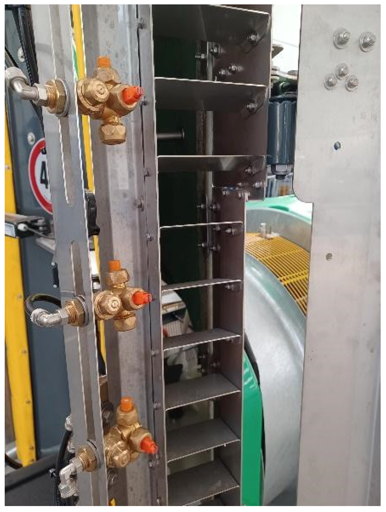
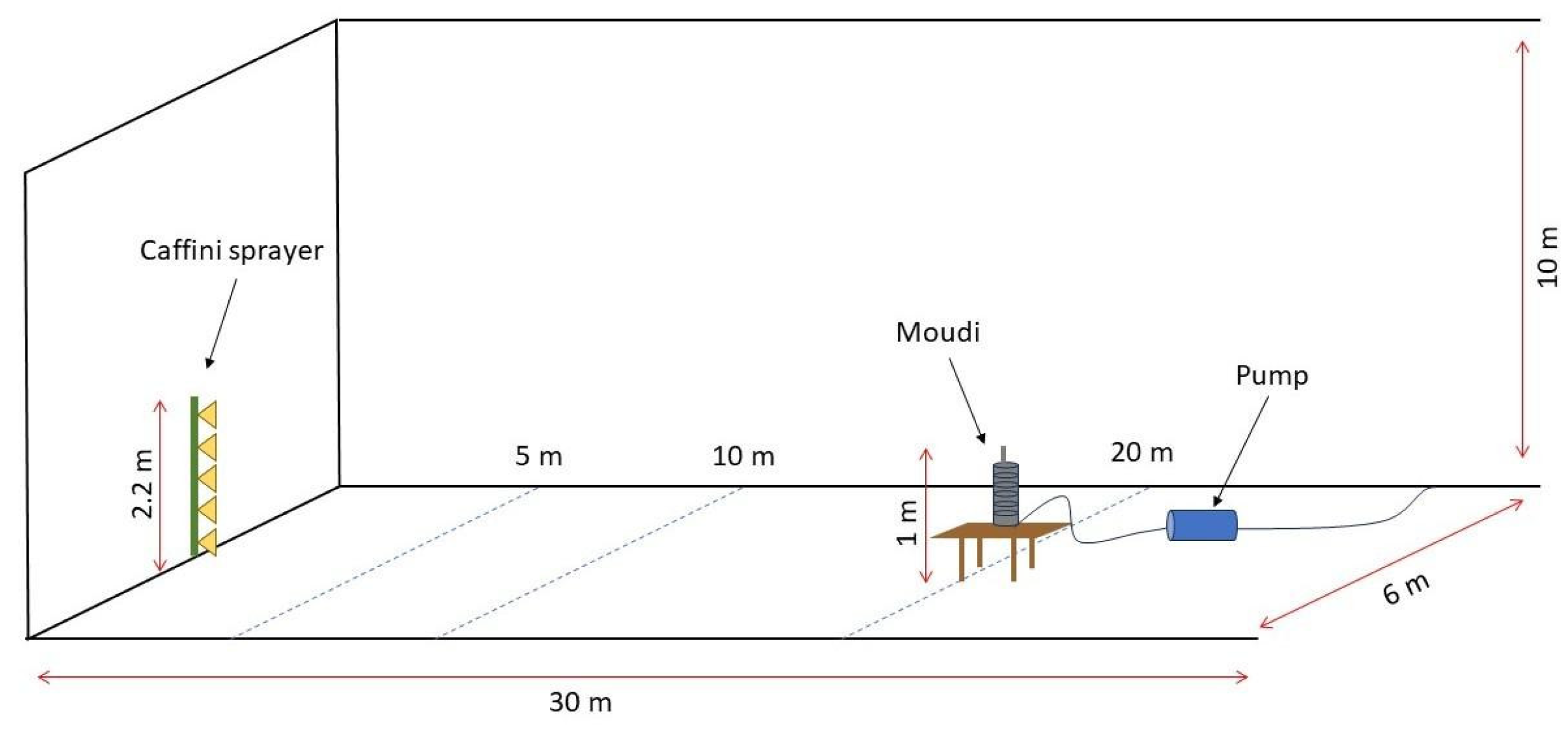
2.2. Experimental Set-Up

All the experiments took place in the wind channel of the Agroforestry Innovations Laboratory of the Free University of Bozen-Bolzano (unibz), installed at the NOI Techpark (Figure 1 and Figure 2). The wind channel, described in detail in [47], enables the testing of entire machines; for the present experiment, it was used as a confined environment without the application of wind. The tunnel is an open channel that is 30 m long, 10 m high, and 6 m wide. The open channel architecture does not recirculate the air and sprayed aerosols; hence, the buildup of leftover aerosols in the test volume is avoided, enabling the quick replacement of the air in the test volume. A Synthesis 1000 sprayer (Caffini s.p.a., Palù, VR, Italy) was used to spray a solution of water and fluorescein at a concentration of 20 mg L−1. Two different sets of nozzles were employed: a conventional hollow cone (henceforth “HC”, model TXB8001VK, Teejet® Technologies, Wheaton, IL, USA) and air inclusion flat fan (henceforth “AI”, model CVI8001, Albuz Spray, Evreux Cedex, France). The delivery pressure was set at 700 kPa, regulated through the manometer available on the machine. The sprayer’s fan was operated at the minimum speed. To select the nozzle specimens to mount on the machine, the flow rate of each candidate specimen was measured in a dedicated test bench. The procedure and the equipment used are outlined in [48]. For each type of nozzle, the 10 which guaranteed the smallest coefficient of variation (CV, defined as the ratio between standard deviation and average) were selected and mounted on the machine. The nominal average flow rates at the selected pressure were 0.57 ± 0.01 L min−1 for HC and 0.600 ± 0.008 L min−1 for AI (mean ± std), meaning CVs of 2.1% and 1.3%, respectively.
Randomly selected specimens of the selected nozzles were then characterized using a particle/droplet image analysis (PDIA) as outlined in the following. The PDIA is a technique which analyzes backlit digital images of a bi-phase flow to count and size the droplets or particles of other types dispersed in the flow. The aerosol sampler used is a 10-stage impactor (Micro-Orifice Uniform Deposit Impactor, MOUDI, Model 110NR, MSP Corporation, Shoreview, MN, USA; Supporting Figure S1), connected to a pump (Gast Manufacturing Inc., Benton Harbor, MI, USA) and with the following size classes: inlet: >18 µm, stage 1: 18 to 10 µm, stage 2: 10 to 5.6 µm, stage 3: 5.6 to 3.2 µm, stage 4: 3.2 to 1.8 µm, stage 5: 1.8 to 1.0 µm, stage 6: 1.0 to 0.56 µm, stage 7: 0.56 to 0.3 2 µm, stage 8: 0.32 to 0.18 µm, stage 9: 0.18 to 0.10 µm, stage 10: 0.10 to 0.056 µm, and backup filter (outlet): <0.056 µm. The sampling flow in each test was 30 L min−1. For every sampling, each plate stage was loaded with a 47 mm disk of aluminum foil, while the outlet that was equipped with a 47 mm quartz filter was previously thermally treated in an oven at 400 °C for 4 h. The sampler was put at 0.70 m height above the ground; thus, the inlet was approximately at 1.0 m from the ground. Prior to every sampling, the MOUDI and the aluminum disks were carefully washed and decontaminated with ultragrade i-PrOH. The aspiration flow was checked before every trial with a flowmeter (Model 6001/Fe, Tecfluid, Sant Just Desvern, Barcelona, Spain) and the proper functioning of the MOUDI was assessed by checking in the control module that the pressure drop across the impactor stages was consistent with the manufacturer’s specifications (Supporting Figure S2). Each test was performed as follows: fluorescein solution was sprayed for 10 min; simultaneously, the sampler was switched on and allowed to sample for the same amount of time (10 min). Next, aluminum disks and the quartz filter were carefully removed from the MOUDI using plastic tweezers, decontaminated with i-PrOH before each filter removal. One by one, the aluminum and quartz disks were put in a 15 mL plastic tube and stored in a freezer (−20 °C) until the analyses. Before each repetition, we operated the wind tunnel’s fan system at full power for a minimum of 5 min, to rid the test volume of leftover aerosols. The sampling was repeated at three different distances, namely 5 m, 10 m, and 20 m from the sprayer, for both nozzles employed. The trial at each distance was repeated three times to assure the repeatability of results. Figure 3 gives a graphical representation of the experimental setup.

2.3. Nozzle Characterization

The drop size distribution (DSD) of the nozzle population was obtained using PDIA at the laboratory located at unibz, where a VisiSize N60 PDIA system is installed (Oxford Lasers, Didcot, Oxfordshire, UK). At least four randomly selected nozzles from each configuration were tested in the dedicated test bench, seen in Figure 4, and described in greater detail in [48,49].
For AI nozzles, the analyses were performed with the specimen spraying down wards in a vertical position, mounting the instrument so that its field of view (FOV) was centered at 30 cm from the orifice, below the nozzle centerline. Previous experiments have shown a good development of the atomization at this distance.
HC nozzles were mounted at a 40° incline from the vertical position, with the spray cone intersecting perpendicularly the instrument’s optical axis at the position of the FOV, 30 cm below the nozzle orifice. The adjustable camera lens was set at the minimum magnification, 0.58×, and the appropriate instrument calibration file was loaded. According to the factory calibration, the minimum droplet area recognizable by the instrument in this configuration is 17 pixels, corresponding to an equivalent diameter of 44.5 µm. Similarly, the maximum equivalent diameter would be close to 4000 µm. The brightness of the back lighting was adjusted to achieve optimal visibility. Figure 5 presents two typical shadowgrams obtained from the HC (top) and AI nozzles (bottom). Tap water at room temperature was sprayed. The pump of the test bench was set at 700 kPa, as would happen on the sprayer. To achieve statistical relevance, a minimum of 15,000 droplets were acquired for each repetition.
The data were extracted from the automatically generated test reports from the VisiSize 6.5.44 software and visualized in MATLAB (The MathWorks, Inc., Natick, MA, USA), readapting the dedicated scripts described in [49]. The main results of the analysis are the DSD of the nozzles, both in terms of number and volume: droplets are classified based on their diameter and, for each class, both the number and the fraction of the total sprayed volume represented by the droplets are recorded. By numerical integration, the number- and volume-based cumulative size distributions (CSDs) can be obtained. The cumulative curves give relevant information about the overall performance of the nozzle, chiefly volume percentiles, relative span, and volume fraction [50]. Volume percentiles dVx represent the diameters which “contain” a specified percentage of the total volume. In short, 10% of the output volume is contained in droplets at most as large in diameter as dV10. Generally, the percentiles recorded and used for comparison are those corresponding to the minimum, middle, and maximum representative fractions, i.e., 10%, 50%, and 90% of the total volume. The 50th is also defined as the Volume Median Diameter (VMD). The relative span (RS) is a measure of how dispersed the DSD is and is calculated as in Equation (1):
RS = (dV90 − dV10)/dV50
The volume fractions Vy are the number of volume percentiles, indicating which proportion of the total volume resides in droplets with a specified diameter. These pieces of information are relevant when estimating the “driftability” of a nozzle: given the size-dependent aerodynamic properties of droplets, the smaller the droplets are, the more they are likely to be transported by wind, in turn increasing the fraction of volume able to drift. There is no clear agreement as to which diameter is to be considered “drift-prone”, but some studies, such as [51], found a satisfying correlation (R2 = 0.948) between the drift potential measured in the field and the V100 of the nozzles (i.e., the fraction of droplets smaller than 100 µm in diameter). This result is in accordance with that of [52].

2.4. Aerosol Chemical Characterization

2.4.1. Preanalytical Treatment and Instrumental Analysis

The extraction of fluorescein from the aluminum disks and quartz filters was performed by first adding 10 mL of a mixture of 9:1 ultrapure water–ultragrade methanol in the 15 mL plastic tube containing the samples, and then by sonicating it in an ultrasound bath for 30 min at room temperature. Fluorescein is not highly water-soluble; on the contrary, it is completely soluble in methanol. To avoid the excessive use of MeOH, which (i) renders the preanalytical treatment less sustainable, (ii) is less safe for the operator, and (iii) notably increases the costs, it was decided to use water and a small amount of an organic polar solvent (methanol) to enhance the extraction efficiency. The supernatant was then filtered in a 1.5 mL glass vial using a 5 mL plastic syringe (Braun, Melsugen, Germany) equipped with a 0.45 µm PTFE filter.
The determination of fluorescein was performed using an Ultimate 3000 UHPLC system (Thermo ScientificTM, Waltham, MA, USA) coupled with a TSQ Altis—Plus Triple Quadrupole Mass Spectrometer (Thermo ScientificTM, Waltham, MA, USA) using a heated-electrospray source (H-ESI). The chromatographic separation was performed using the Agilent Zorbax SB C18 2.1 × 150 3.5 µm. The mobile phase used during the elution was a mixture of ultrapure water (phase A) and methanol (phase B), with a flow rate of 0.300 mL min−1. The chromatographic run was set as follows: 0–0.8 min isocratic step at 10% phase B; 0.8–1.5 min gradient from 10% to 100% phase B; 1.5–5 min isocratic step at 100% phase B; and 5–6 min equilibration stage at 10% B. The injection volume was set at 20 µL. The mass spectrometer’s source parameters were set as follows: negative potential −2300 V; sheath gas 50 Arb; auxiliary gas 5 Arb; sweep gas 0 Arb; ion transfer tube temperature 250 °C; and vaporizer temperature 400 °C. Data were collected in multiple-reaction monitoring (MRM) mode, and two MRM transitions were analyzed: the most intense (331 > 286 m/z, CE 20, RF-Lens 80) was used for quantification, while the other (331 > 243, CE 25, RF-lens 80) was used to confirm the compound identity. All the data are collected in Tables S1 and S2.

2.4.2. Method Validation (AQ/CQ)

The analytical procedure was validated by determining the instrumental linear ranges, procedural blanks, method detection and quantification limits (MDL and MQL), repeatability, and trueness for aluminum and quartz filters. The instrumental response showed a linear range between 0.1 and 9 µg L−1, with an R2 value of 0.9999. The mean blank values are checked for aluminum (0.02 µg L−1) and quartz (0.02 µg L−1) filters by the analysis of three filters extracted using the procedure described above. The MDL and MQL were quantified as three times the standard deviation of the average values of the blank (n = 3) for both types of filters. The values of MDL were 0.03 µg L−1 and 0.02 µg L−1, while the MQLs were 0.1 µg L−1 and 0.08 µg L−1 for aluminum and quartz filters, respectively. Due to the lack of certified reference materials for fluorescein in aerosol or dust, we estimated trueness and repeatability by analyzing three spiked cleaned filters with 100 abs ng of fluorescein. The trueness was evaluated as the difference between the mean values and the ‘true’ values spiked, obtaining a weak underestimate (−4%) for the aluminum filter and a weaker overestimation (+3%) for the quartz filter (reported as percent errors). The method precision in terms of repeatability was calculated using the relative standard deviation (RSD%) by consecutive measurements of the spiked samples (n = 3). The values were 4% and 7% for aluminum and quartz filters, respectively. All the data are summarized in Table S3.

3. Results and Discussion

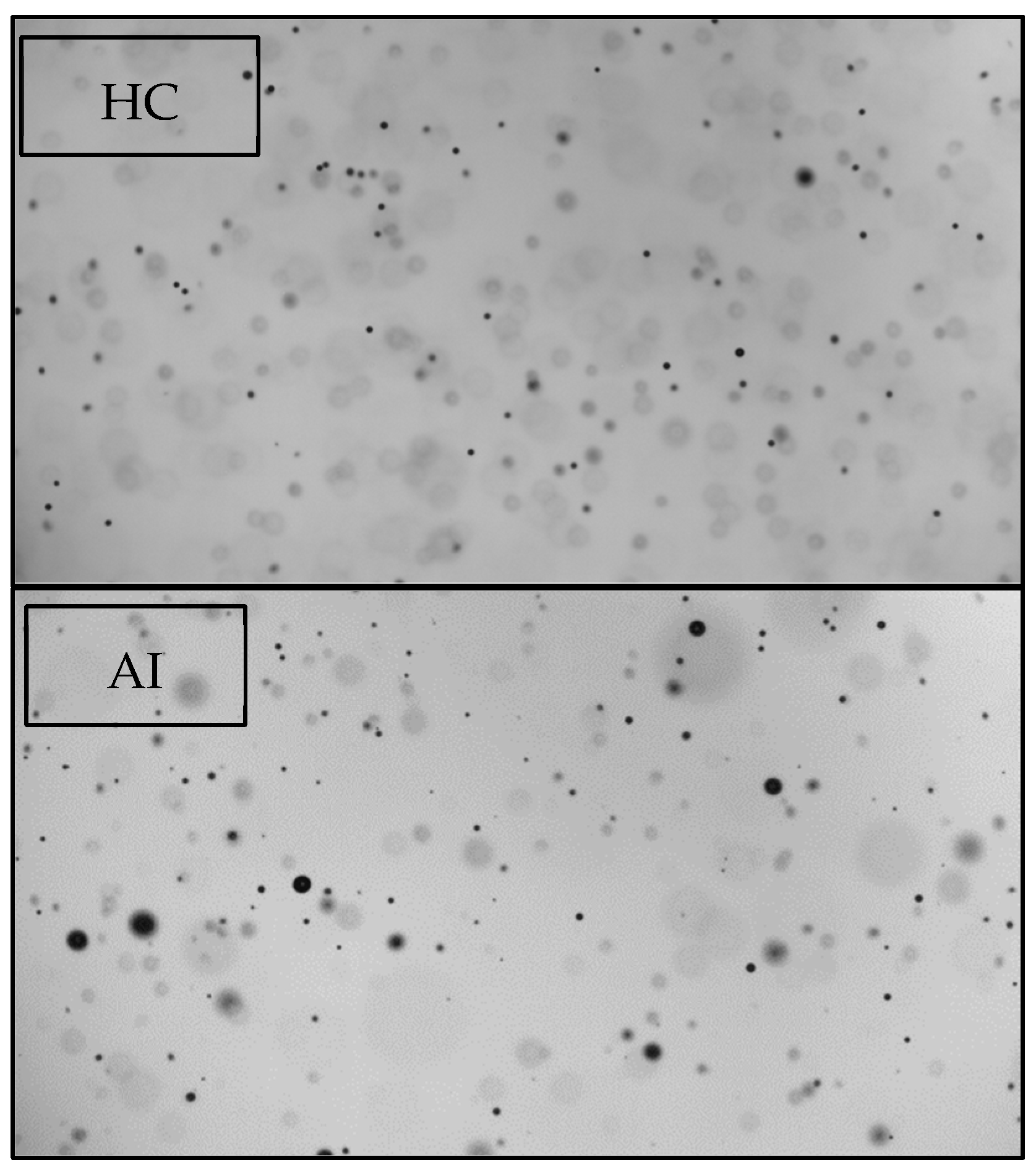
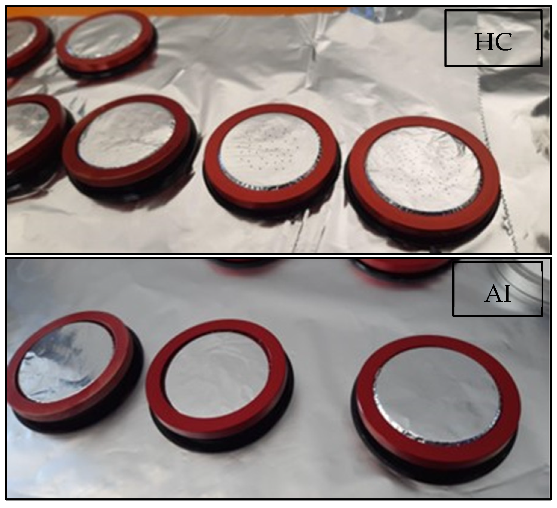
3.1. Nozzle Optical Analyses (Particles Larger Than 40 µm)

The characterization of nozzles shows significant agreement among nozzles of the same type, confirming the validity of the configuration mounted on the sprayer. Table 1 reports the averages (avgs), standard deviations (stds), and the coefficients of variations (CVs) of the nozzle types.
Only the V100 from the HC nozzle shows a considerable variation: this could be due to different reasons, including the inherent variability in the mass manufacturing of nozzles. However, this hypothesis, together with the hypothesis concerning mistakes in setting up the instrument, appear unlikely: the nozzles were all tested in a single session, and the other results agree considerably.
At the smaller end of the spectra, the first statistically significant diameters (dV10) appear to be equivalent for the two nozzles. However, the two nozzles distribute volumes in much different ways, with the VMD of the AI nozzle being more than double than that of the HC nozzle, and the dV90 being significantly higher. This is in accordance with the working of the two nozzle types. The characterization, visualized in Figure 6, clearly presents the two nozzle types as working according to their purpose: the conventional HC nozzles prove very precise in generating narrow droplet spectra (RS < 1), while the air inclusion into droplets proves to be a more chaotic process, generating a wide spectrum of droplets. This spectrum contains an important share of much larger droplets. Although not as frequent as the smaller ones, these larger classes carry a significantly higher share of volume, as can be seen in the volume-based DSD in Figure 6, right. The height of the classes in this second histogram does not represent the sheer count of droplets belonging to the class, but rather the share of total disbursed volume contained in droplets of the class. This information is much more significant, in that it shows how the output volume is distributed across the spectrum, and hence how much of this volume is more likely to drift. This shifting of the histogram is not so relevant for the HC nozzle due to its limited span, but it is quite visible for the AI nozzle.

3.2. Chemical Analyses (Particle Range 0.056 to 40 µm)

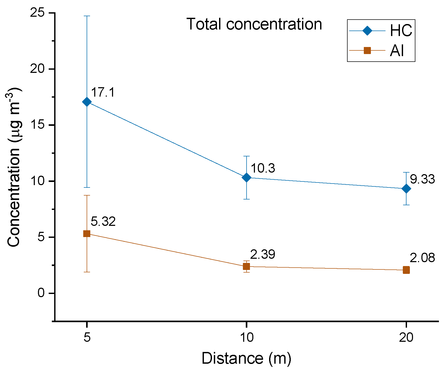
3.2.1. Total Concentration Trend and Stages

The different behavior of AI and HC nozzles was immediately observed from a qualitative point of view. First, the spray produced by the HC nozzle was more visible and similar to a thick fog compared to the one produced by the AI nozzle. Second, when the aluminum disks were removed from the cascade impactor stages after the HC experiment, fluorescein was visibly deposited on the substrate (the dark spots in Figure 7, top). On the contrary, the disks exposed to the AI repetitions showed only a small presence of the marker (Figure 7, bottom), hardly visible to the naked eye. For every test performed (two types of nozzles and three distances from the sprayer), the total concentration of fluorescein was calculated by summing the concentration of all size ranges. The results are in accordance with the qualitative evidence mentioned above (Figure 8). Indeed, the HC profile of the total concentration shows a notable presence of fluorescein at 5 m from the sprayer (17 ± 7 µg m−3), while the AI profile reaches a much lower total concentration (5 ± 3 µg m−3) at the same distance. Although AI and HC nozzles have a similar volume of solution distributed per minute (as per Section 2.2), the AI nozzle notably reduced marker dispersion. This evidence can be explained by the different workings of the nozzles and the greater abatement of coarse particles by the AI nozzle within the first 5 m. Indeed, the PDIA analysis has demonstrated not only that the AI nozzle produces bigger droplets compared to the HC nozzle, but that the largest amount of volume of the solution is disbursed by AI nozzles in the form of coarser droplets than those of HC nozzles. In addition, the inclusion of air causes a reduction in fluid power due to energy lost to mixing; therefore, the AI droplets will tend to fall sooner with respect to the HC droplets.
In the HC nozzle trials, the fluorescein concentration decreases between 10 and 20 m, although less dramatically as compared to the decrease from 5 m to 10 m. A similar trend is also visible for the AI repetitions. Overall, from 5 to 20 m there is a reduction of fluorescein concentration of 46% and 61% when using HC and AI nozzles, respectively. This evidence again confirms the hypotheses reported above. Overall, the total concentrations differ notably, although for both AI and HC experiments, there is a similar descending trend in fluorescein concentration as the distance from the sprayer increases. Note that the standard deviation for the HC trials is much higher compared to the AI trials.
The use of a cascade impactor allowed us to study the dimensional distribution of the droplet produced by the two nozzles. Starting from the first distance (5 m), as can be seen from Figure 9, the HC and the AI nozzles have a similar size distribution pattern, with the fraction > 18 µm (inlet) being dominant in terms of marker concentration and the finer fractions (stages 7-outlet, 0.056–0.56 µm) being almost negligible. This evidence is coherent with the proximity of the sampler to the source, and highlights that the coarser fraction distributions of HC and AI nozzles behave similarly at this distance. In all the size ranges, the HC concentration is higher than that of the AI concentration. When the distance is increased to 10 m, the trend of AI droplets again mimics the trend of the HC nozzles, although (i) the concentration of marker is consistently reduced and (ii) there are specific size ranges that present some differences. Indeed, the concentration in stage S2 of the AI experiments is slightly higher than in the HC experiments, and the amount of fluorescein at the outlet is much higher in the HC experiments compared to the AI experiments. There is a remarkable abatement of the coarser fraction (inlet) for both the AI (from 4 ± 3 µg m−3 to 0.3 ± 0.2 µg m−3) and HC experiments (10 ± 8 µg m−3 to 2.1 ± 0.5 µg m−3), while the concentration starts to increase in stages S2–S6 compared to the 5 m. At the maximum distance from the sprayer (20 m), both nozzle trials show an abatement of all coarser particles (inlet and S1), and the fine fraction starts to rise in concentration (S7-outlet). Compared to previous distances, at 20 m the trend of AI and HC droplets differs more, as the maximum concentration value is reached in stage S4 for the HC experiments, while in the AI experiments, it is reached at stage S3 (5.6–3.2 µm), and as the amount of the finest fraction (<0.056 µm) in the HC experiments increases notably. This means that a remarkable number of driftable particles are still present at 20 m when HC nozzles are employed.

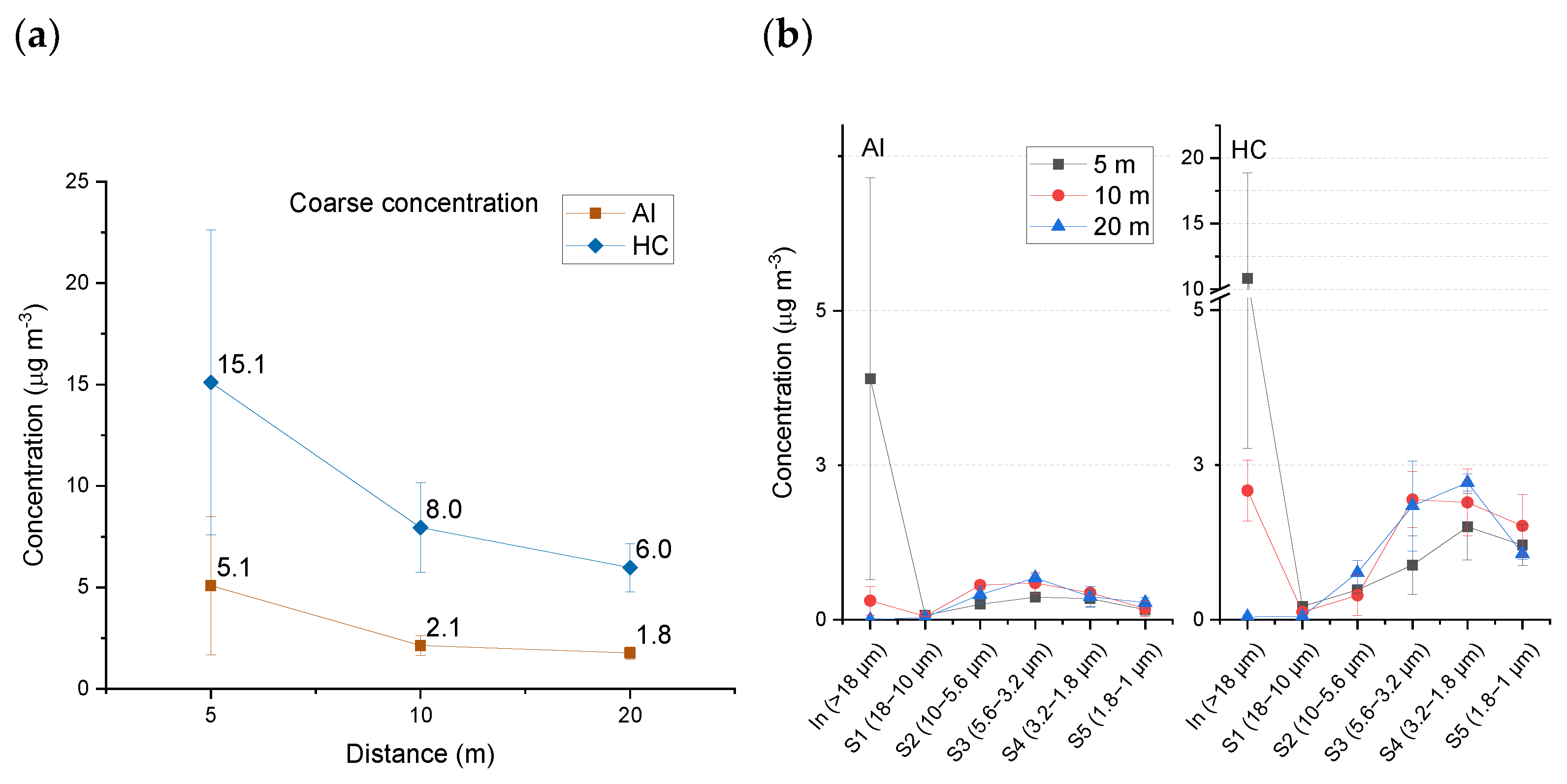
3.2.2. Coarse Fractions (Stages S Inlet–S5)

Interesting results can be obtained by splitting the total concentrations found for both nozzles in the corresponding contributions of coarse and fine particles (Figure 10a,b and Figure 11a,b, respectively). As can be seen, the two scenarios change notably. For what concerns the coarse class (>18–1 µm, corresponding to inlet to S5 of the multistage impactor), AI and HC nozzles share a similar decreasing trend as the distance increases, in accordance with the trend of the total concentration (Figure 10a).
Indeed, it was expected that the coarser fractions would have a greater effect on the total concentration compared to the finer fractions, as they carry a higher amount of marker. This trend is particularly coherent to the AI nozzles’ behavior reported in Figure 6, where the majority of the volume disbursed is contained in coarse particles. For both the nozzles trials, at the distance of 5 m (Figure 10b) the maximum marker concentration is observed at the inlet (>18 µm), which then has a solid decrease at 10 m and disappears at 20 m. Stage S1 is almost negligible, while stage S2 shows a different trend for the AI and HC nozzles: indeed, for the former there are three distinct values for each distance, with 10 m being the highest, but for the latter, concentrations are closer to one another. Overall, the smallest fractions (S2–S5) begin to increase when distance increases. Together with the decrease in total coarse particles concentrations, this evidence might suggest that, from 5 m to 10 m, the large droplets tend to fall and/or to evaporate, leaving smaller droplets, as the droplet size is also dependent on atmospheric conditions (i.e., evaporation) [17]. Moreover, the peak of concentrations in the AI trials ranges between S2 and S3, while for the HC trials, it ranges between S3 and S4. This evidence is in accordance with the working mechanism of the AI nozzle, which, by including air in the drop, creates larger droplets, and with the PDIA measurements. At 20 m, the HC droplet shows a profile rich in S4 fractions.

3.2.3. Fine Fractions (Stages S6-Out)
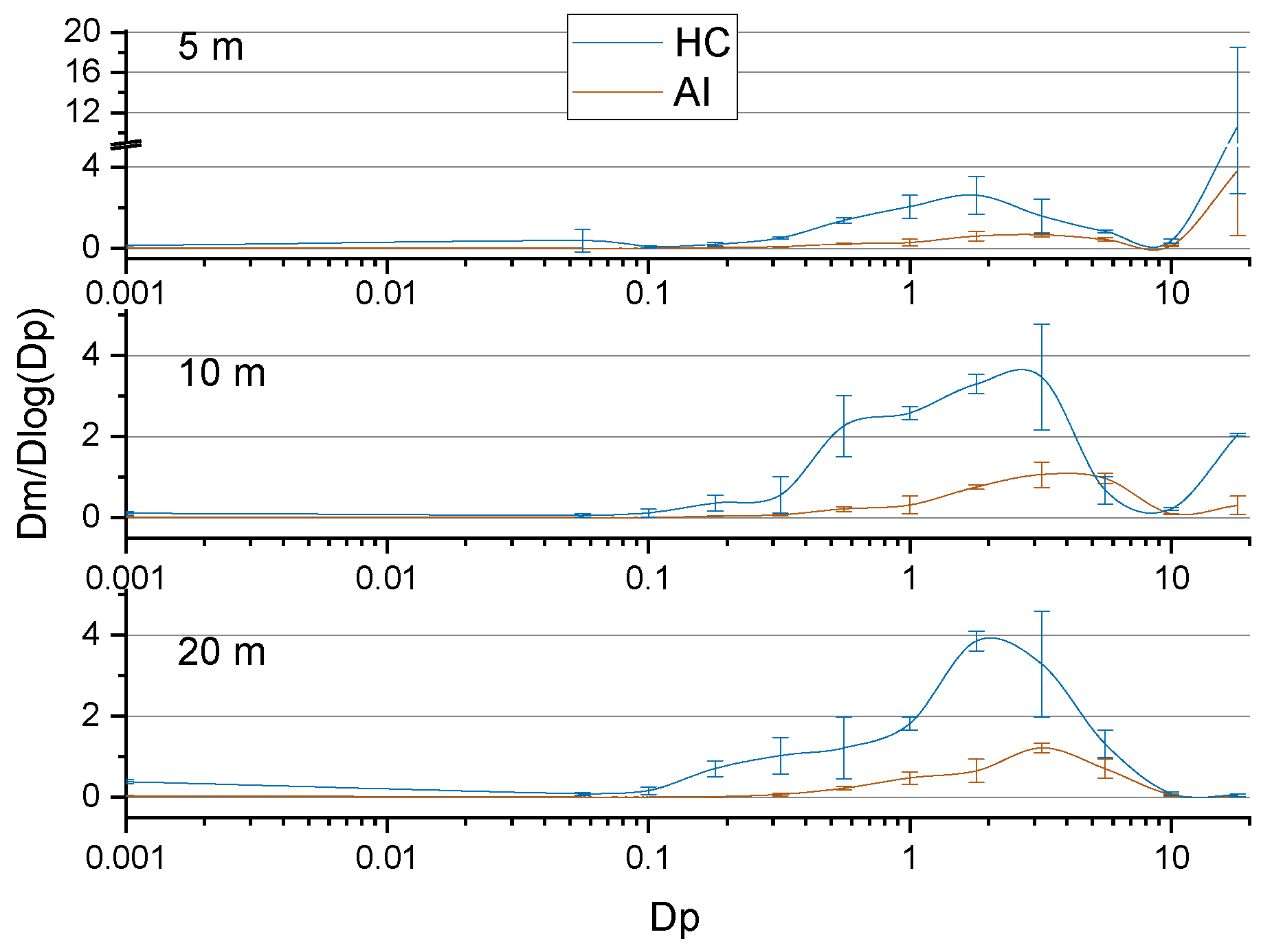
As mentioned above, the behavior of finer fractions (corresponding to stages S6-Out) produced by the AI and HC nozzles is remarkably different. By looking at Figure 11a, it is evident how the finest fractions are almost completely abated by the AI nozzle, compared to the HC nozzle, which on the contrary produces a notable number of fine droplets. This might seem contradictory to Figure 6, which shows that the AI nozzle produces a higher number of fine particles. We can conclude that the amount of solution that these droplets bring to the sampler is much less compared to the HC spray. For both nozzles, the concentration of S6-outlet particles increases with distance, but the concentration for HC nozzles at 20 m is 2.6 ± 0.3 µg m−3, almost fifteen times higher than the marker concentration dispensed by the AI nozzles at the same experimental conditions. The minor presence of finer fractions at 10 m of the HC trials is in accordance with the major presence of bigger fractions, as reported above in the coarse section. Regarding the specific stages, Figure 11b highlights how the AI trials follow a more organized trend while the HC trend is more irregular. The AI droplet profile of 5 m and 10 m show an almost equal pattern in stages S6–S10. Looking at the final stage, the AI nozzle follows a directly proportional trend, as the more the distance increases, the higher the presence of the finer fraction. Nevertheless, the amount of fluorescein is almost an order of magnitude less than the same stage, at 20 m, in the HC droplet. Another piece of evidence is that in the AI profile, stages 9 and 10 are always below the detection limit, while the HC nozzle shows a small, but present, concentration of fluorescein.

3.2.4. Modes

A conclusive view on the particle size distribution can be obtained by plotting modes for both the nozzles at different distances. As evident from Figure 12, the coarser fraction, above 10 µm in diameter, tends to disappear from 5 m to 20 m, while smaller particles tend to remain almost constant, with a small increment. This seems to support the thesis of the partial evaporation of the biggest droplets during the route from the emission point to the last sampling spot. The different function of the AI and HC nozzles is evident when looking at the distance of 10 m and 20 m: indeed, the trend of the former is located principally in the coarse area (>1 µm), while the latter is more shifted toward the fine fraction.

4. Conclusions

The work herein presented focuses on the evaluation of PPP drift produced by a full-scale orchard sprayer equipped with two types of nozzles, namely an anti-drift flat fan (AI) nozzle and a conventional hollow cone (HC) nozzle, in a semi-controlled environment. The biggest fractions of the droplets (>40 µm) were evaluated using particle/droplet image analysis (PDIA) at the outlet of the nozzles, while the smallest (<40 µm) were sampled with a cascade impactor at 5 m, 10 m, and 20 m from the emission point and analyzed using a new and fast HPLC-MS/MS method. Fluorescein was used as chemical marker to simulate the phytosanitary product. PDIA analyses showed a good consistency in behavior among nozzles of the same type, with the HC nozzle being accurate at producing sharp drop size distributions (DSDs) with a very limited statistical dispersion. In turn, AI nozzles produce a much wider DSD spectrum, concentrating the largest part of the distributed volume into droplets of larger size. The HPLC-MS/MS analysis demonstrated that the AI nozzle remarkably reduces the dispersion of fluorescein in the air compared to the HC nozzle, and the abatement of the finer droplets was confirmed, especially at 20 m. Concentration trends have shown the similarity between coarse fractions and total concentration behavior, while the trends of fine fractions are strongly different. Overall, this study provides solid information on the characterization of droplets sprayed by HC and AI nozzles and on the size distribution of aerosol droplets produced by the two nozzles at specific distances. The novelty of the presented approach, beside the usage of an entire machine in its field configuration, lies in the integration of different instrumental approaches. This can provide a key to developing reliable testing practices to improve the quality certification of new machinery, and to assess the overall impact of plant protection campaigns to ensure the spreading of good practices. Further studies are needed to evaluate how the aerosol distribution pattern changes when parameters like wind, spray pressure, and obstacles are modified to mimic real conditions.

Supplementary Materials

The following supporting information can be downloaded at: https://www.mdpi.com/article/10.3390/atmos15060656/s1, Figure S1: The 10-stage cascade impactor (MOUDI) employed for the sampling in the wind chamber; Figure S2: Flowmeter employed for the correct performance measure of the cascade impactor; Table S1: Instrumental parameters for fluorescein analysis; Table S2: MS/MS filter parameter for native compound fluorescein; Table S3: Values of blank, MDL, MQL, recovery, trueness, and precision for fluorescein extraction procedure validation, expressed as the relative percentage standard deviation (RSD%).

Author Contributions

Conceptualization, L.B., G.M., A.A., M.B., E.G., M.F., E.B., D.C., F.M. and A.G.; formal analysis, L.B., G.M., A.A., M.B., E.G., M.F., E.B. and D.C.; investigation, L.B., G.M., A.A., M.B., E.G., M.F., E.B., D.C. and A.G.; resources, L.B., G.M., A.A., M.B., E.G. and F.M.; visualization, L.B. and G.M.; writing—original draft, L.B. and G.M.; writing—review and editing, L.B., G.M., A.A., M.B., E.G., M.F., E.B., D.C., F.M. and A.G. All authors have read and agreed to the published version of the manuscript.

Funding

This research received no external funding.

Institutional Review Board Statement

Not applicable.

Informed Consent Statement

Not applicable.

Data Availability Statement

All data will be made available upon request. The code for the MATLAB scripts is available at GitHub (https://github.com/SpaceLoreB/N60-Post-Processing).

Acknowledgments

The authors would like to thank Caffini s.p.a. for the provision of the sprayer, the Consorzio Agrario di Bolzano/Landwirtschaftliche Hauptgenossen schaft Sudtirol for the provision of the tractor and the laboratory technicians of unibz J. Zelger, D. Klammer, and M. Malavasi for the technical support for the experiment. This research has been carried out within the PNRR research activities of the consortium iNEST (Interconnected North-East Innovation Ecosys tem), funded by the European Union Next-GenerationEU (Piano Nazionale di Ripresa e Resilienza (PNRR)–Missione 4 Componente 2, Investimento 1.5–D.D. 1058 23/06/2022, ECS 00000043). Line of research: Spoke 1-Ecosystems for Mountain Innovations, RT1B (Safety and Life Quality in Mountain Habitat). This manuscript only reflects the authors’ views and opinions; neither the European Union nor the European Commission can be considered responsible for them. This work has benefited from the infrastructural support of the Centre for Trace Analysis (CeTrA) of Ca’ Foscari University through the project IR0000032–ITINERIS, Italian Integrated Environmental Research Infrastructures System, funded by EU-Next Generation EU, PNRR-Mission 4 “Education and Research”-Component 2: “From research to business” Investment 3.1: “Fund for the realisation of an integrated system of research and innovation infrastructures”.

Conflicts of Interest

The authors declare no conflicts of interest.

References

  1. Pogacean, M.; Gavrilescu, M. Plant Protection Products and Their Sustainable and Environmentally Friendly Use. Environ. Eng. Manag. J. 2009, 8, 607–627. [Google Scholar] [CrossRef]
  2. Betarbet, R.; Sherer, T.B.; MacKenzie, G.; Garcia-Osuna, M.; Panov, A.V.; Greenamyre, J.T. Chronic Systemic Pesticide Exposure Reproduces Features of Parkinson’s Disease. Nat. Neurosci. 2000, 3, 1301–1306. [Google Scholar] [CrossRef] [PubMed]
  3. Contini, D.; Cesari, D.; Genga, A.; Siciliano, M.; Ielpo, P.; Guascito, M.R.; Conte, M. Source Apportionment of Size-Segregated Atmospheric Particles Based on the Major Water-Soluble Components in Lecce (Italy). Sci. Total Environ. 2014, 472, 248–261. [Google Scholar] [CrossRef] [PubMed]
  4. Damalas, C.A.; Eleftherohorinos, I.G. Pesticide Exposure, Safety Issues, and Risk Assessment Indicators. Int. J. Environ. Res. Public Health 2011, 8, 1402–1419. [Google Scholar] [CrossRef] [PubMed]
  5. Liu, Q.; Chen, S.; Wang, G.; Lan, Y. Drift Evaluation of a Quadrotor Unmanned Aerial Vehicle (UAV) Sprayer: Effect of Liquid Pressure and Wind Speed on Drift Potential Based on Wind Tunnel Test. Appl. Sci. 2021, 11, 7258. [Google Scholar] [CrossRef]
  6. Mostafalou, S.; Abdollahi, M. Pesticides and Human Chronic Diseases: Evidences, Mechanisms, and Perspectives. Toxicol. Appl. Pharmacol. 2013, 268, 157–177. [Google Scholar] [CrossRef] [PubMed]
  7. Muñoz, J.P.; Silva-Pavez, E.; Carrillo-Beltrán, D.; Calaf, G.M. Occurrence and Exposure Assessment of Glyphosate in the Environment and Its Impact on Human Beings. Environ. Res. 2023, 231, 116201. [Google Scholar] [CrossRef] [PubMed]
  8. Directive 2009/128/EC of the European Parliament and of the Council of 21 October 2009 Establishing a Framework for Community Action to Achieve the Sustainable Use of Pesticides Text with EEA Relevance. 2009. Available online: http://data.europa.eu/eli/dir/2009/128/2009-11-25 (accessed on 28 May 2024).
  9. Matthews, G.A. Application of Pesticides to Crops; World Scientific Publishing Company: Singapore, 1999; ISBN 978-1-911298-12-0. [Google Scholar]
  10. Wang, G.; Han, Y.; Li, X.; Andaloro, J.; Chen, P.; Hoffmann, W.C.; Han, X.; Chen, S.; Lan, Y. Field Evaluation of Spray Drift and Environmental Impact Using an Agricultural Unmanned Aerial Vehicle (UAV) Sprayer. Sci. Total Environ. 2020, 737, 139793. [Google Scholar] [CrossRef]
  11. Singh, N.K.; Sanghvi, G.; Yadav, M.; Padhiyar, H.; Christian, J.; Singh, V. Fate of Pesticides in Agricultural Runoff Treatment Systems: Occurrence, Impacts and Technological Progress. Environ. Res. 2023, 237, 117100. [Google Scholar] [CrossRef] [PubMed]
  12. Felsot, A.S.; Unsworth, J.B.; Linders, J.B.H.J.; Roberts, G.; Rautman, D.; Harris, C.; Carazo, E. Agrochemical Spray Drift; Assessment and Mitigation—A Review. J. Environ. Sci. Health Part B 2010, 46, 1–23. [Google Scholar] [CrossRef] [PubMed]
  13. Samsonov, Y.N.; Makarov, V.I.; Koutsenogii, K.P.; Raputa, V.F. Wind Drifts of Pesticide Aerosols after Various Methods of Pesticide Application. J. Aerosol Sci. 1998, 29, S177–S178. [Google Scholar] [CrossRef]
  14. Holterman, H.J.; van de Zande, J.C.; Porskamp, H.A.J.; Huijsmans, J.F.M. Modelling Spray Drift from Boom Sprayers. Comput. Electron. Agric. 1997, 19, 1–22. [Google Scholar] [CrossRef]
  15. Kira, O.; Linker, R.; Dubowski, Y. Estimating Drift of Airborne Pesticides during Orchard Spraying Using Active Open Path FTIR. Atmos. Environ. 2016, 142, 264–270. [Google Scholar] [CrossRef]
  16. Miller, P. The Measurement of Spray Drift. Pest. Outlook 2003, 14, 205. [Google Scholar] [CrossRef]
  17. Precipito, L.M.B.; Ferreira, L.A.I.; Paduan, N.A.; Lima, J.S.d.S.; de Oliveira, R.B. Use of the Test Bench for Spray Drift Assessment under Subtropical Climate Conditions. Rev. Bras. Eng. Agrícola E Ambient. 2022, 27, 223–229. [Google Scholar] [CrossRef]
  18. Butler Ellis, M.C.; Lane, A.G.; O’Sullivan, C.M.; Jones, S. Wind Tunnel Investigation of the Ability of Drift-Reducing Nozzles to Provide Mitigation Measures for Bystander Exposure to Pesticides. Biosyst. Eng. 2021, 202, 152–164. [Google Scholar] [CrossRef]
  19. Grant, S.; Perine, J.; Abi-Akar, F.; Lane, T.; Kent, B.; Mohler, C.; Scott, C.; Ritter, A. A Wind-Tunnel Assessment of Parameters That May Impact Spray Drift during UAV Pesticide Application. Drones 2022, 6, 204. [Google Scholar] [CrossRef]
  20. Nuyttens, D.; Zwertvaegher, I.K.A.; Dekeyser, D. Spray Drift Assessment of Different Application Techniques Using a Drift Test Bench and Comparison with Other Assessment Methods. Biosyst. Eng. 2017, 154, 14–24. [Google Scholar] [CrossRef]
  21. Chen, S.; Lan, Y.; Zhou, Z.; Ouyang, F.; Wang, G.; Huang, X.; Deng, X.; Cheng, S. Effect of Droplet Size Parameters on Droplet Deposition and Drift of Aerial Spraying by Using Plant Protection UAV. Agronomy 2020, 10, 195. [Google Scholar] [CrossRef]
  22. Kira, O.; Dubowski, Y.; Linker, R. In-Situ Open Path FTIR Measurements of the Vertical Profile of Spray Drift from Air-Assisted Sprayers. Biosyst. Eng. 2018, 169, 32–41. [Google Scholar] [CrossRef]
  23. Ling, W.; Du, C.; Ze, Y.; xindong, N.; Shumao, W. Research on the Prediction Model and Its Influencing Factors of Droplet Deposition Area in the Wind Tunnel Environment Based on UAV Spraying. IFAC-PapersOnLine 2018, 51, 274–279. [Google Scholar] [CrossRef]
  24. Krogh, K.A.; Halling-Sørensen, B.; Mogensen, B.B.; Vejrup, K.V. Environmental Properties and Effects of Nonionic Surfactant Adjuvants in Pesticides: A Review. Chemosphere 2003, 50, 871–901. [Google Scholar] [CrossRef] [PubMed]
  25. Mesnage, R.; Benbrook, C.; Antoniou, M.N. Insight into the Confusion over Surfactant Co-Formulants in Glyphosate-Based Herbicides. Food Chem. Toxicol. 2019, 128, 137–145. [Google Scholar] [CrossRef] [PubMed]
  26. Castro, M.J.L.; Ojeda, C.; Cirelli, A.F. Advances in Surfactants for Agrochemicals. Environ. Chem. Lett. 2014, 12, 85–95. [Google Scholar] [CrossRef]
  27. Cornacchia, I.; Tomas, S.; Douzals, J.-P.; Courault, D. Assessment of Airborne Transport of Potential Contaminants in a Wind Tunnel. J. Irrig. Drain. Eng. 2020, 146, 04019031. [Google Scholar] [CrossRef]
  28. Grella, M.; Miranda-Fuentes, A.; Marucco, P.; Balsari, P. Field Assessment of a Newly-Designed Pneumatic Spout to Contain Spray Drift in Vineyards: Evaluation of Canopy Distribution and off-Target Losses. Pest Manag. Sci. 2020, 76, 4173–4191. [Google Scholar] [CrossRef]
  29. Wang, C.; Wongsuk, S.; Huang, Z.; Yu, C.; Han, L.; Zhang, J.; Sun, W.; Zeng, A.; He, X. Comparison between Drift Test Bench and Other Techniques in Spray Drift Evaluation of an Eight-Rotor Unmanned Aerial Spraying System: The Influence of Meteorological Parameters and Nozzle Types. Agronomy 2023, 13, 270. [Google Scholar] [CrossRef]
  30. Kjær, C.; Bruus, M.; Bossi, R.; Løfstrøm, P.; Andersen, H.V.; Nuyttens, D.; Larsen, S.E. Pesticide Drift Deposition in Hedgerows from Multiple Spray Swaths. J. Pestic. Sci. 2014, 39, 14–21. [Google Scholar] [CrossRef]
  31. Makhnenko, I.; Alonzi, E.R.; Fredericks, S.A.; Colby, C.M.; Dutcher, C.S. A Review of Liquid Sheet Breakup: Perspectives from Agricultural Sprays. J. Aerosol Sci. 2021, 157, 105805. [Google Scholar] [CrossRef]
  32. ISO 10625; Equipment for Crop Protection—Sprayer Nozzles—Colour Coding for Identification. International Standards Organisation (ISO): Geneva, Switzerland, 2018.
  33. Carvalho, T.C.; Peters, J.I.; Williams, R.O. Influence of Particle Size on Regional Lung Deposition—What Evidence Is There? Int. J. Pharm. 2011, 406, 1–10. [Google Scholar] [CrossRef]
  34. National Research Council. Breathing, Deposition, and Clearance. In Comparative Dosimetry of Radon in Mines and Homes; National Academies Press (US): Washington, DC, USA, 1991. [Google Scholar]
  35. Hatch, T.F. Distribution and Deposition of Inhaled Particles in Respiratory Tract. Bacteriol. Rev. 1961, 25, 237–240. [Google Scholar] [CrossRef] [PubMed]
  36. Jabbal, S.; Poli, G.; Lipworth, B. Does Size Really Matter?: Relationship of Particle Size to Lung Deposition and Exhaled Fraction. J. Allergy Clin. Immunol. 2017, 139, 2013–2014.e1. [Google Scholar] [CrossRef]
  37. Suarez-Lopez, J.R.; Nazeeh, N.; Kayser, G.; Suárez-Torres, J.; Checkoway, H.; López-Paredes, D.; Jacobs, D.R.; de la Cruz, F. Residential Proximity to Greenhouse Crops and Pesticide Exposure (via Acetylcholinesterase Activity) Assessed from Childhood through Adolescence. Environ. Res. 2020, 188, 109728. [Google Scholar] [CrossRef] [PubMed]
  38. Pascuzzi, S.; Manetto, G.; Santoro, F.; Cerruto, E. A Brief Review of Nozzle Spray Drop Size Measurement Techniques. In Proceedings of the 2021 IEEE International Workshop on Metrology for Agriculture and Forestry (MetroAgriFor), Trento-Bolzano, Italy, 3–5 November 2021; pp. 351–355. [Google Scholar]
  39. Grella, M.; Maffia, J.; Dinuccio, E.; Balsari, P.; Miranda-Fuentes, A.; Marucco, P.; Gioelli, F. Assessment of Fine Droplets (<10 Μm) in Primary Airborne Spray Drift: A New Methodological Approach. J. Aerosol Sci. 2023, 169, 106138. [Google Scholar] [CrossRef]
  40. Kashdan, J.T.; Shrimpton, J.S.; Whybrew, A. Two-Phase Flow Characterization by Automated Digital Image Analysis. Part 2: Application of PDIA for Sizing Sprays. Part. Part. Syst. Charact. 2004, 21, 15–23. [Google Scholar] [CrossRef]
  41. Kashdan, J.T.; Shrimpton, J.S.; Whybrew, A. Two-Phase Flow Characterization by Automated Digital Image Analysis. Part 1: Fundamental Principles and Calibration of the Technique. Part. Part. Syst. Charact. 2003, 20, 387–397. [Google Scholar] [CrossRef]
  42. Cooper, J.F.; Smith, D.N.; Dobson, H.M. An Evaluation of Two Field Samplers for Monitoring Spray Drift. Crop Prot. 1996, 15, 249–257. [Google Scholar] [CrossRef]
  43. Coscollà, C.; Muñoz, A.; Borrás, E.; Vera, T.; Ródenas, M.; Yusà, V. Particle Size Distributions of Currently Used Pesticides in Ambient Air of an Agricultural Mediterranean Area. Atmos. Environ. 2014, 95, 29–35. [Google Scholar] [CrossRef]
  44. Coscollà, C.; Yahyaoui, A.; Colin, P.; Robin, C.; Martinon, L.; Val, S.; Baeza-Squiban, A.; Mellouki, A.; Yusà, V. Particle Size Distributions of Currently Used Pesticides in a Rural Atmosphere of France. Atmos. Environ. 2013, 81, 32–38. [Google Scholar] [CrossRef]
  45. Radoman, N.; Christiansen, S.; Johansson, J.H.; Hawkes, J.A.; Bilde, M.; Cousins, I.T.; Salter, M.E. Probing the Impact of a Phytoplankton Bloom on the Chemistry of Nascent Sea Spray Aerosol Using High-Resolution Mass Spectrometry. Environ. Sci. Atmos. 2022, 2, 1152–1169. [Google Scholar] [CrossRef]
  46. Ware, G.W.; Estesen, B.J.; Cahill, W.P.; Gerhardt, P.D.; Frost, K.R. Pesticide Drift. I. High-Clearance vs. Aerial Application of Sprays. J. Econ. Entomol. 1969, 62, 840–843. [Google Scholar] [CrossRef]
  47. Becce, L.; Carabin, G.; Mazzetto, F. Agroforestry Innovations Lab Activities on Sprayer Performance and Certification. In Proceedings of the AIIA 2022: Biosystems Engineering Towards the Green Deal, Palermo, Italy, 19–22 September 2022; pp. 305–313. [Google Scholar]
  48. Becce, L.; Mazzi, G.; Ali, A.; Bortolini, M.; Gambaro, A.; Mazzetto, F. Nozzle Characterisation to Support Aerosol Spray Drift Measurement in a Semi-Controlled Environment. In Proceedings of the 2023 IEEE International Workshop on Metrology for Agriculture and Forestry (MetroAgriFor), Pisa, Italy, 6 November 2023; pp. 646–651. [Google Scholar]
  49. Becce, L.; Amin, S.; Carabin, G.; Mazzetto, F. Preliminary Spray Nozzle Characterization Activities through Shadowgraphy at the AgroForestry Innovation Lab (AFI-Lab). In Proceedings of the 2022 IEEE Workshop on Metrology for Agriculture and Forestry (MetroAgriFor), Perugia, Italy, 3 November 2022; pp. 136–140. [Google Scholar]
  50. Lefebvre, A.H.; McDonell, V.G. Atomization and Sprays, 2nd ed.; CRC Press; Taylor & Francis Group: Boca Raton, FL, USA, 2017; ISBN 978-1-4987-3625-1. [Google Scholar]
  51. Torrent, X.; Gregorio, E.; Douzals, J.-P.; Tinet, C.; Rosell-Polo, J.R.; Planas, S. Assessment of Spray Drift Potential Reduction for Hollow-Cone Nozzles: Part 1. Classification Using Indirect Methods. Sci. Total Environ. 2019, 692, 1322–1333. [Google Scholar] [CrossRef] [PubMed]
  52. Arvidsson, T.; Bergström, L.; Kreuger, J. Spray Drift as Influenced by Meteorological and Technical Factors: Spray Drift as Influenced by Meteorological and Technical Factors. Pest Manag. Sci. 2011, 67, 586–598. [Google Scholar] [CrossRef] [PubMed]
Figure 1. The wind tunnel where the experiments took place.
Atmosphere 15 00656 g001
Figure 2. A close-up view of the sprayer outlet duct with air outlet and nozzle holders equipped with the two types of nozzles mounted.
Atmosphere 15 00656 g002
Figure 3. Scheme of the experimental setup. The sprayer, equipped with AI or HC nozzles (yellow), was put at the beginning of the wind chamber; the impactor was put on a table at a specific distance from the sprayer (5 m, 10 m, and 20 m).
Atmosphere 15 00656 g003
Figure 4. The test bench installed in the laboratory with (1) multimeter, (2) nozzle mount, (3) optical setup of the shadowgraph, and (4) collection tubs. From [49].
Atmosphere 15 00656 g004
Figure 5. Shadows of droplets from HC (top) and AI (bottom) nozzles when analyzed using the PDIA.
Atmosphere 15 00656 g005
Figure 6. DSD of the two nozzle types by number (left) and volume (right).
Atmosphere 15 00656 g006
Figure 7. Aluminum disks of the same cascade impactor stages after sampling spray produced by the HC nozzles (top) and spray produced by the AI nozzles (bottom). The dots are stains of fluorescein.
Atmosphere 15 00656 g007
Figure 8. Total concentration of fluorescein, calculated as the sum of all the stages at a certain distance, for each nozzle.
Atmosphere 15 00656 g008
Figure 9. Concentration of fluorescein depending on nozzle type, stages, and distance. Bars represent the standard deviation.
Atmosphere 15 00656 g009
Figure 10. Total coarse concentration (a) and size-segregated coarse concentration (b) for HC and AI nozzles. The vertical bars represent the standard deviation.
Atmosphere 15 00656 g010
Figure 11. Total fine concentration (a) and size-segregated fine concentration (b) for HC and AI nozzles. The vertical bars represent the standard deviation. The vertical bars represent the standard deviation.
Atmosphere 15 00656 g011
Figure 12. Comparison of AI and HC nozzles modes, at the distance of 5 m, 10 m, and 20 m. The vertical bars represent the standard deviation.
Atmosphere 15 00656 g012
Table 1. Characterization results for the hollow cone (HC) and air inclusion (AI) nozzles.
HCAI
Avg ± stdCV (%)Avg ± stdCV (%)
dV10 [µm]98 ± 56109 ± 44
dV50 [µm]114 ± 65286 ± 114
dV90 [µm]150 ± 128530 ± 163
RS0.46 ± 0.08111.47 ± 0.055
V100 [%]12 ± 12998 ± 113
V200 [%]99 ± 1133 ± 27
Disclaimer/Publisher’s Note: The statements, opinions and data contained in all publications are solely those of the individual author(s) and contributor(s) and not of MDPI and/or the editor(s). MDPI and/or the editor(s) disclaim responsibility for any injury to people or property resulting from any ideas, methods, instructions or products referred to in the content.

