Numerical Simulation and Risk Assessment of Cascade Reservoir Dam-Break

Abstract
:1. Introduction
2. Methods
2.1. Simulation of Single-Embankment Dam-Break
2.1.1. Dam-Break Outflow
2.1.2. Vertical Erosion of the Breach
2.1.3. Lateral Enlargement of the Breach
2.2. Flood Routing Simulation (FRS)
2.3. Flood-Regulating Calculation (FRC)
2.4. Cascade Reservoir Breaching Simulation (CRBS)
3. Results and Discussion
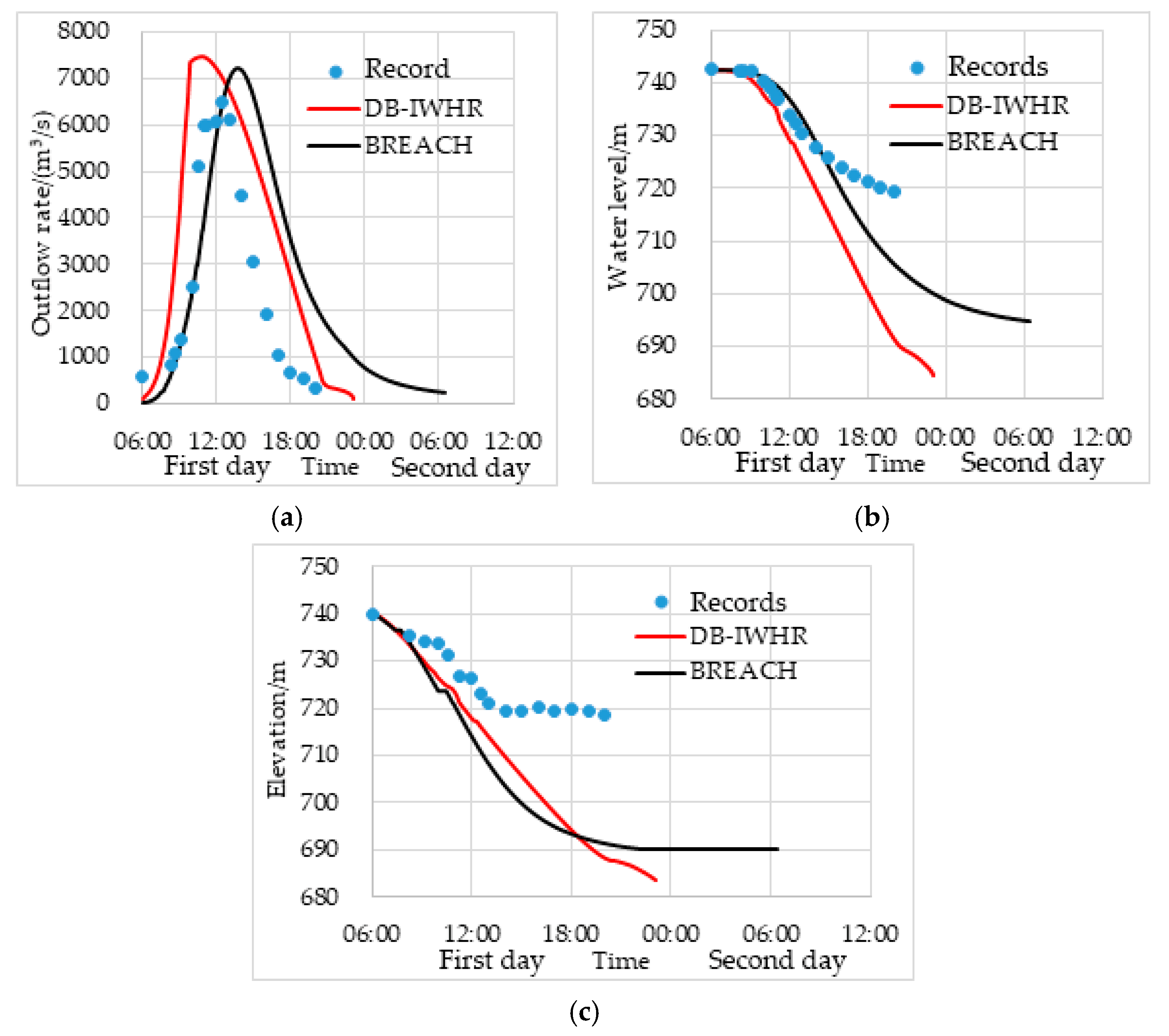
3.1. Dam-Break of Tangjiashan Barrier Lake
3.2. Flood Routing in The Middle Riverway
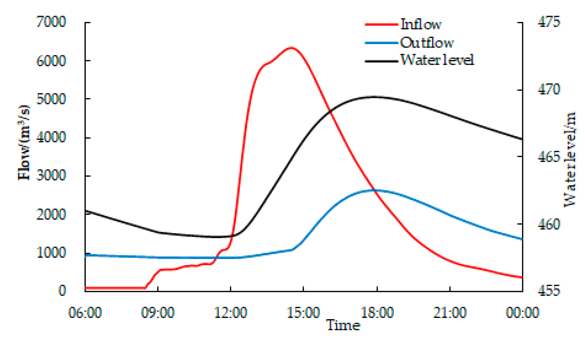
3.3. Flood Regulation in the Downstream Reservoir
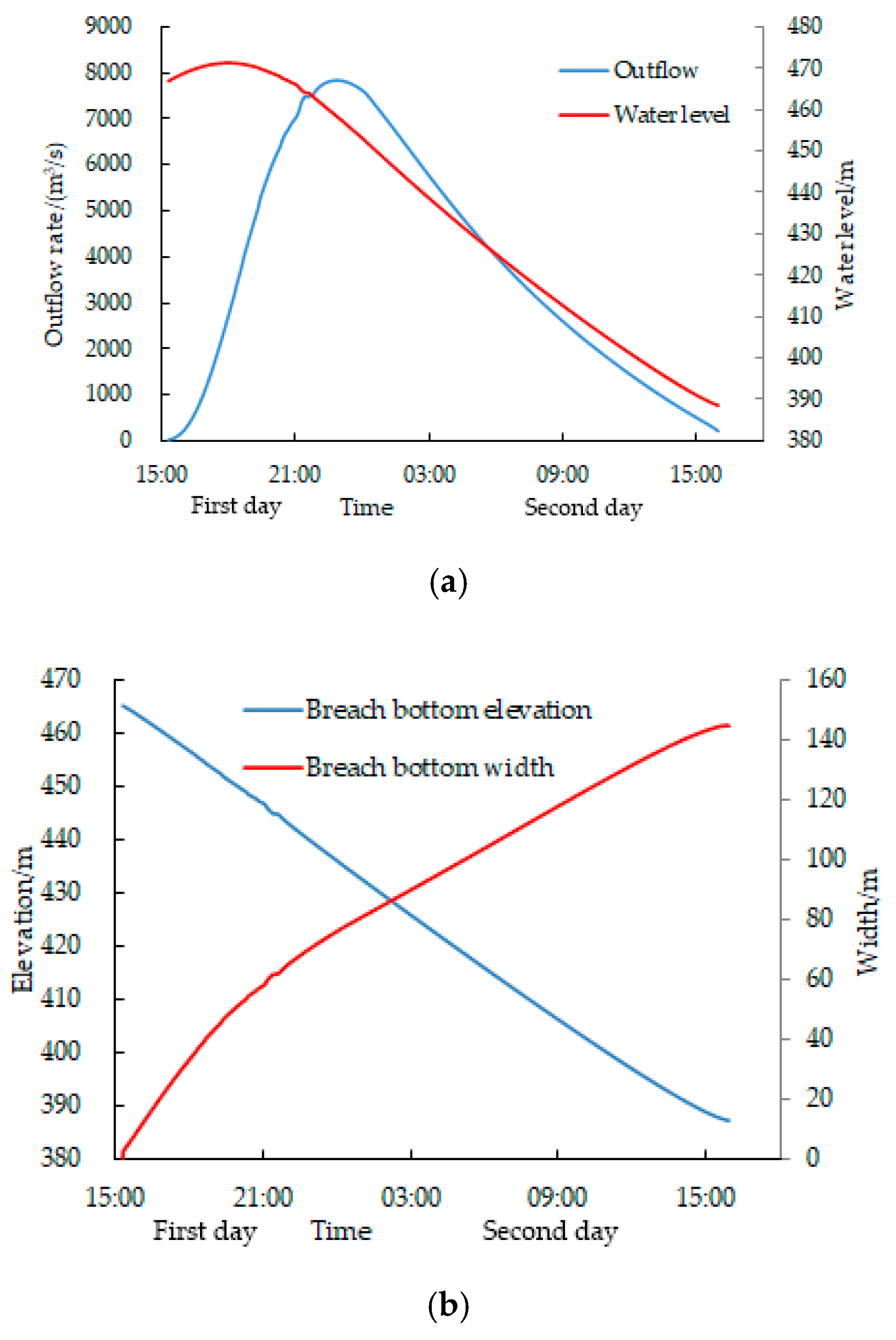
3.4. Sequential Break of Downstream Dam II
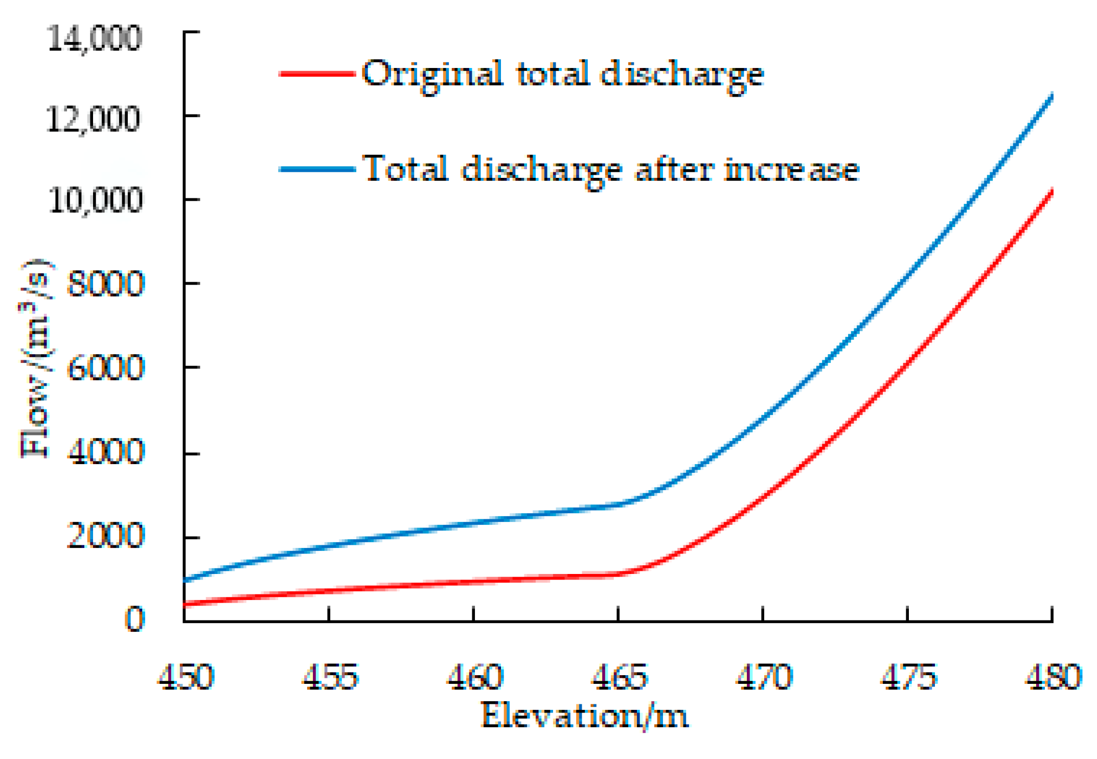
3.5. Risk Analysis of Reservoir II under Different Operating Schemes
4. Conclusions
Author Contributions
Funding
Conflicts of Interest
References
- Mohamed, A.R.; Lee, K.T. Energy for sustainable development in Malaysia: Energy policy and alternative energy. Energy Policy 2006, 34, 2388–2397. [Google Scholar] [CrossRef]
- Cai, W.; Zhu, X.; Peng, A.; Wang, X.; Fan, Z. Flood risk analysis for cascade dam systems: A case study in the Dadu River Basin in China. Water 2019, 11, 1365. [Google Scholar] [CrossRef] [Green Version]
- Bernardo, N.; Alcântara, E.; Watanabe, F.; Rodrigues, T.; Carmo, A.D.; Gomes, A.C.C.; Andrade, C. Light absorption budget in a reservoir cascade system with widely differing optical properties. Water 2019, 11, 229. [Google Scholar] [CrossRef] [Green Version]
- Zhou, J.; Zhou, X.; Du, X.; Wang, F. Research on design of dam-break risks control for cascade reservoirs. Shuili Fadian Xuebao/J. Hydroelectr. Eng. 2018, 37, 1–10. [Google Scholar]
- Wetmore, J.N.; Fread, D.L. The NWS Simplified Dam-Break Flood Forecasting Model; National Weather Service: Silver Spring, MD, USA, 1991. [Google Scholar]
- Shi, Z.M.; Guan, S.G.; Peng, M.; Zhang, L.M.; Zhu, Y.; Cai, Q.P. Cascading breaching of the Tangjiashan landslide dam and two smaller downstream landslide dams. Eng. Geol. 2015, 193, 445–458. [Google Scholar] [CrossRef]
- Xue, Y.; Xu, W.; Luo, S.; Chen, H.; Li, N.; Xu, L. Experimental study of dam-break flow in cascade reservoirs with steep bottom slope. J. Hydrodyn. 2011, 23, 491–497. [Google Scholar] [CrossRef]
- Niu, Z.; Xu, W.; Li, N.; Xue, Y.; Chen, H. Experimental Investigation of the Failure of Cascade Landslide Dams. J. Hydrodyn. 2012, 24, 430–441. [Google Scholar] [CrossRef]
- Cao, Z.; Huang, W.; Pender, G.; Liu, X. Even more destructive: Cascade dam break floods. J. Flood Risk Manag. 2014, 7, 357–373. [Google Scholar] [CrossRef]
- Zhou, J.; Wang, H.; Chen, Z.; Zhou, X.; Li, B. Evaluations on the safety design standards for dams with extra height or cascade impacts. Part I: Fundamentals and criteria. Shuili Xuebao/J. Hydraul. Eng. 2015, 46, 505–514. [Google Scholar]
- Bouchehed, H.; Mihoubi, M.K.; Derdous, O.; Djemili, L. Evaluation of potential dam break flood risks of the cascade dams mexa and bougous (El Taref, Algeria). J. Water Land Dev. 2017, 33, 39–45. [Google Scholar] [CrossRef] [Green Version]
- Zhang, S.; Tan, Y. Risk assessment of earth dam overtopping and its application research. Nat. Hazards 2014, 74, 717–736. [Google Scholar] [CrossRef]
- Zhu, Y.; Visser, P.; Vrijling, J. Review on Embankment Dam Breach Modeling. New Developments in Dam Engineering; Taylor & Francis Group: Abingdon, UK, 2004; pp. 1189–1196. [Google Scholar]
- Singh, V.P.; Scarlatos, P.D. Analysis of gradual earth-dam failure. J. Hydraul. Eng. 1988, 114, 21–42. [Google Scholar] [CrossRef]
- Brown, R.J.; Rogers, D.C. BRDAM User’s Manual; Water and Power Resources Service: Denver, CO, USA, 1981. [Google Scholar]
- Singh, V.P.; Scarlatos, P.D.; Collins, J.G.; Jourdan, M.R. Breach Erosion of Earthfill Dams (BEED) model. Nat. Hazards 1988, 1, 161–180. [Google Scholar] [CrossRef]
- Fread, D.L. BREACH: An Erosion Model for Earthen Dam Failures; National Weather Service: Silver Spring, MD, USA, 1988. [Google Scholar]
- Brunner, G. HEC-RAS River Analysis System, Hydraulic Reference Manual, Version 4.1; U.S. Army Engineer Hydrologic Engineering Center: Davis, CA, USA, 2010.
- DHI. MIKE11: A Modeling System for Rivers and Channels User-Guide Manual; Danish Hysraulic Institute: Horsholm, Denmark, 2005. [Google Scholar]
- Li, X.; Chen, Z. Comparison of two models for back analysis of dam breach of Tangjiashan Barrier Lake. Adv. Sci. Technol. Water Resour. 2017, 37, 20–26. [Google Scholar]
- Alaghmand, S.; Abdullah, R.B.; Abustan, I.; Eslamian, S. Comparison between Capabilities of HEC-RAS and MIKE-11 hydraulic models in river flood risk modelling (a case study of Sungai Kayu Ara River Basin, Malaysia). Int. J. Hydrol. Sci. Technol. 2012, 2, 270. [Google Scholar] [CrossRef]
- You, L.; Li, C.; Min, X.; Xiaolei, T. Review of dam-break research of earth-rock dam combining with dam safety management. Procedia Eng. 2012, 28, 382–388. [Google Scholar] [CrossRef] [Green Version]
- Chen, Z.; Ma, L.; Yu, S.; Chen, S.; Zhou, X.; Sun, P.; Li, X. Back analysis of the draining process of the Tangjiashan Barrier Lake. J. Hydraul. Eng. 2015, 141, 1–14. [Google Scholar] [CrossRef]
- Chen, S.; Wang, Q.; Yu, S.; Wang, H. Comparative analysis of models for overtopping-induced earth-rock dam breach. J. Hohai Univ. 2016, 44, 406–411. [Google Scholar]
- Singh, V.P. Dam Breaching Modeling Technology; Kluwer Academic Publishers: Dordrecht, The Netherlands, 1996. [Google Scholar]
- Chen, Z.Y. Soil Slope Stability Analysis Principles Methods; Water and Power Press: Beijing, China, 2003. [Google Scholar]
- Bishop, A.W. The use of the slip circle in the stability analysis of slopes. Géotechnique 1955, 5, 7–17. [Google Scholar] [CrossRef]
- Moussa, R.; Bocquillon, C. Criteria for the choice of flood-routing methods in natural channels. J. Hydrol. 1996, 186, 1–30. [Google Scholar] [CrossRef]
- Fenton, J.D. Reservoir routing. Hydrol. Sci. J. 1992, 37, 233–246. [Google Scholar] [CrossRef]
- Chen, S.Y. Numerical solution method and procedure for reservoir routing. Shuili Xuebao/J. Hydraul. Eng. 1980, 2, 44–49. [Google Scholar]
- Liu, N.; Zhang, J.; Lin, W.; Cheng, W.; Chen, Z. Draining Tangjiashan Barrier Lake after Wenchuan earthquake and the flood propagation after the dam break. Sci. China Ser. E Technol. Sci. 2009, 52, 801–809. [Google Scholar] [CrossRef]
- Hu, X.; Huang, R.; Shi, Y.; Lu, X.; Zhu, H.; Wang, X. Analysis of blocking river mechanism of tangjiashan landslide and dam-breaking mode of its barrier dam. Yanshilixue Yu Gongcheng Xuebao/Chin. J. Rock Mech. Eng. 2009, 28, 181–189. [Google Scholar]
- Liu, N.; Chen, Z.; Zhang, J.; Lin, W.; Chen, W.; Xu, W. Draining the Tangjiashan Barrier Lake. J. Hydraul. Eng. 2010, 136, 914–923. [Google Scholar] [CrossRef]


| Dam Crest Elevation (m) | Dam Height (m) | Check Flood Level (m) | Normal Pool Level (m) | Dead Water Level (m) | Total Storage (×108 m3) | Dead Storage (×108 m3) |
|---|---|---|---|---|---|---|
| 465 | 113.5 | 462.6 | 461 | 445 | 2.763 | 1.615 |
| Category | Parameters | Sign (Unit) | Value |
|---|---|---|---|
| Parameters of dam body | Dam crest elevation | z0 (m) | 740 |
| Initial inflow | qi (m3/s) | 80 | |
| Basis flooding level | Hr (m) | 700 | |
| Initial width of the breach | B0 (m) | 14.4 | |
| Initial slope of the breach | J | 1.2 | |
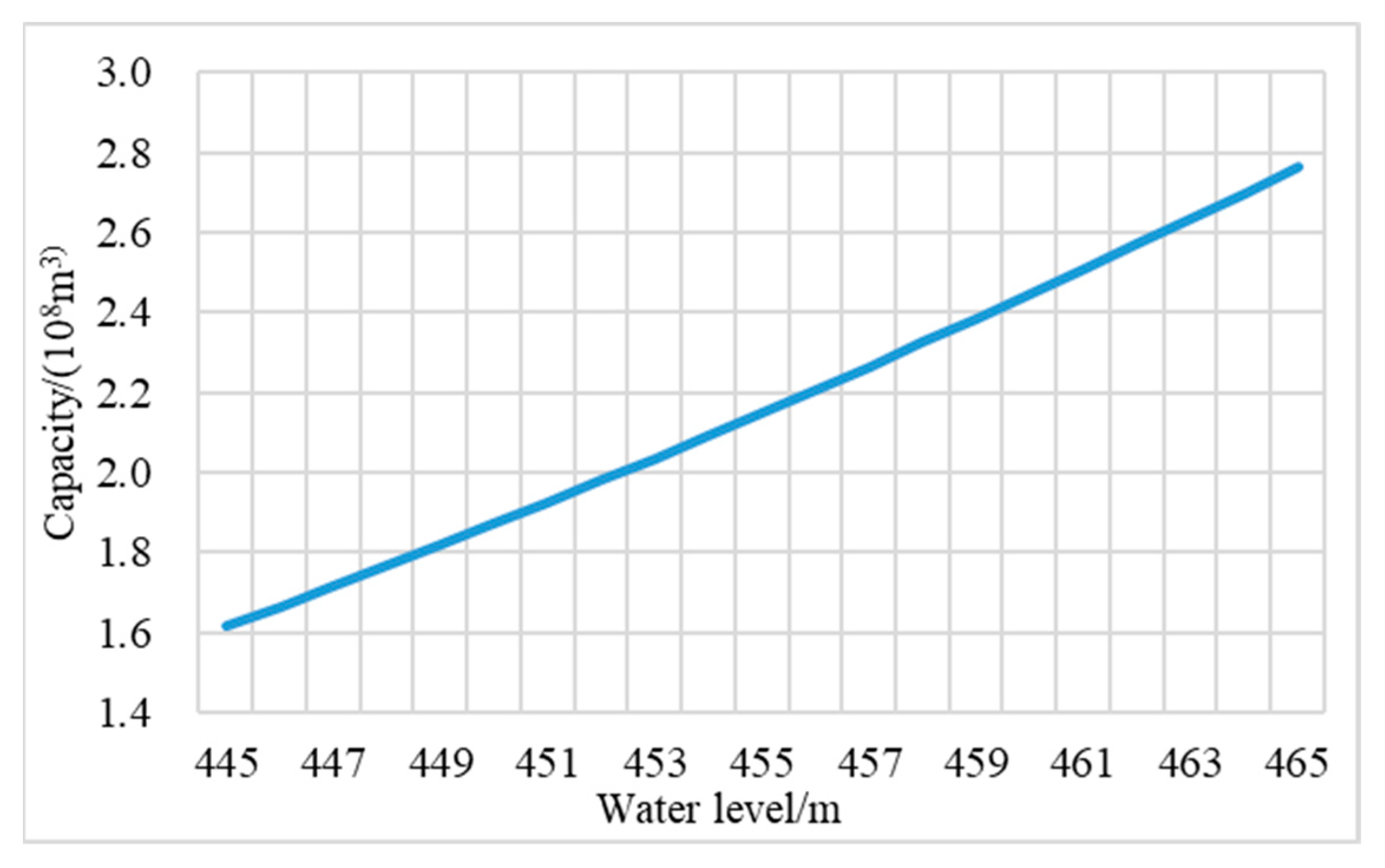
| Parameters of reservoir capacity | Fitting coefficients of water level-storage | a, b, c | 0.06, 1.96, 44 |
| Parameters of weir flow | Discharge coefficient | C1 | 1.43 |
| Submergence coefficient | C2 | 0.94 | |
| Correction ratio for head loss | m | 0.80 | |
| Parameters of erosion | Initial erosion velocity | Vc (m/s) | 2.7 |
| Fitting coefficients of erosion rate | a2, b2 | 1.1, 0.0005 | |
| Shear strength | Cu (kPa) | 25 | |
| Internal friction angle | ϕu (°) | 26 |
| Category | Parameters (Unit) | Value |
|---|---|---|
| Parameters of dam body | Initial water level (m) | 742.5 |
| Dam crest elevation (m) | 742.5 | |
| Dam bottom elevation (m) | 669.5 | |
| Upstream slope | 4 | |
| Downstream slope | 1.2 | |
| Dam crest length (m) | 400 | |
| Manning coefficient | 0.0177 | |
| Parameters of material property | Grain diameter (mm) | 5 |
| Specific gravity | 2.65 | |
| Porosity | 0.43 | |
| Cohesive force (kPa) | 25 | |
| Internal friction angle (°) | 26 | |
| Coefficient of material discontinuity | 30 |
| Category | Parameters | Sign (Unit) | Value |
|---|---|---|---|
| Parameters of dam body | Dam crest elevation | z0 (m) | 465 |
| Initial inflow | qi (m3/s) | 232 | |
| Basis flooding level | Hr (m) | 445 | |
| Initial width of the breach | B0 (m) | 0.0 | |
| Parameters of reservoir capacity | Fitting coefficients of water level-storage | a, b, c | 0.04, 4.94, 161.49 |
| Parameters of weir flow | Discharge coefficient | C1 | 0.36 |
| Submergence coefficient | C2 | 0.90 | |
| Correction ratio for head loss | m | 0.67 | |
| Parameters of erosion | Initial erosion velocity | Vc (m/s) | 3.0 |
| Fitting coefficients of erosion rate | a2, b2 | 1.10, 0.001 |
© 2020 by the authors. Licensee MDPI, Basel, Switzerland. This article is an open access article distributed under the terms and conditions of the Creative Commons Attribution (CC BY) license (http://creativecommons.org/licenses/by/4.0/).
Share and Cite
Hu, L.; Yang, X.; Li, Q.; Li, S. Numerical Simulation and Risk Assessment of Cascade Reservoir Dam-Break. Water 2020, 12, 1730. https://doi.org/10.3390/w12061730
Hu L, Yang X, Li Q, Li S. Numerical Simulation and Risk Assessment of Cascade Reservoir Dam-Break. Water. 2020; 12(6):1730. https://doi.org/10.3390/w12061730
Chicago/Turabian StyleHu, Liangming, Xu Yang, Qian Li, and Shuyu Li. 2020. "Numerical Simulation and Risk Assessment of Cascade Reservoir Dam-Break" Water 12, no. 6: 1730. https://doi.org/10.3390/w12061730