Abstract
Land Surface Temperature (LST) is an important climate factor for understanding the relationship between the land surface and atmosphere. Furthermore, LST is linked to soil moisture and evapotranspiration, which can potentially alter the severity and regime of wildfires, landslide-triggering precipitation thresholds, and others. In this paper, the monthly daytime and nighttime LST products of Moderate Resolution Imaging Spectroradiometer (MODIS) are employed for the period 2000–2023 in order to find areas that have been cooling or warming in a region of great interest in Central Italy, due to its complex geological and geomorphological settings and its recent seismic sequences and landslide events. The annual MODIS land cover images for 2001–2022 are also utilized to investigate the interconnection between LST and land cover change. The results of the non-parametric Mann–Kendall trend test and its associated Sen’s slope reveal a significant nighttime warming trend in the region, particularly in July, linked to forest and woodland expansion. Grasslands toward the coastline with low elevation (less than 500 m a.s.l.) have experienced significant heat waves during the summer, with an LST of more than 35 °C. A significant negative correlation between the elevation and LST is observed for each calendar month. In particular, the daytime and nighttime LST have more than 80% correlation with elevation during winter and summer, respectively. In addition, nighttime warming and gradual drainage are noticed in Lake Campotosto. The results of this study could be useful for wildfire and landslide susceptibility analyses and hazard management.
1. Introduction
Land Surface Temperature (LST), the radiative skin temperature of the land, is a very important climate variable that shows how hot or cold the Earth’s surface is [1]. LST is highly sensitive to vegetation density, and can vary significantly from day to night, and vice versa, based on land cover and altitude [2,3]. LST is significantly correlated with soil moisture over large areas, and is used for many purposes, such as monitoring of droughts, surface water and groundwater, and studies concerning slope stability and landslides [4,5,6].
In situ LST measurements can be obtained accurately and continuously over time; however, such measurements are not acquired for the entire landscape, and are limited to station locations [7,8]. Satellite-based LST products have become a reliable source for monitoring the LST at local, regional, and global scales [8]. Currently, there are many satellite sensors that acquire LST; however, cloud cover can result in a significant missing LST data [7,8,9]. The Moderate Resolution Imaging Spectroradiometer (MODIS) instrument, operating on both Terra and Aqua satellites, acquires day and night LST with an accuracy of 1 K under clear-sky conditions [7,10]. Terra, launched in December 1999, passes though the Equator at 10:30 and 22:30, and Aqua, launched in May 2002, passes through Equator at 1:30 and 13:30 (times are approximate and in local solar time)—both satellites are sun-synchronous, polar-orbiting, and are flying at altitude of about 705 km [11].
Daytime and nighttime MODIS–LST products have been utilized in many studies. Eleftheriou et al. [12] utilized these products for 2000–2017, and estimated the annual and seasonal trends across Greece using the Ordinary Least-Squares (OLS) fitting. They observed a warming annual trend in the nighttime LST more significantly in the southeastern parts of Greece. Waring et al. [13] estimated linear trends of the Aqua MODIS–LST time series by OLS fitting for nine regions, including the Amazon, Australia, China, Greenland, India, the Sahel, Siberia, Western Europe, and the USA during 2002–2021. They showed that the Amazon and Western USA have significant warming daytime LST trends, and Western Europe and USA show the largest nighttime change. Siddiqui et al. [14] employed MODIS-LST images from 2001 to 2018, and showed that nighttime LST is a better indicator for studying urban heating effects for Indian cities. They applied the non-parametric Mann–Kendall trend test, and its associated Sen’s slope estimator (MK–Sen), to estimate the daytime and nighttime LST trends. They observed an annual warming trend for day and night in all Indian cities except Pune. In another study, Shawky et al. [15] analyzed the MODIS daytime and nighttime LST from 2000 to 2021 for the ecoregions of South Asia using MK–Sen, and discussed the interconnection between land cover and cooling/warming trends.
The OLS and MK–Sen are popular methods of trend analysis for hydrometeorological time series; however, caution should be exercised when applying either of these methods [8]. Sen’s slope is based on a median approach, which is less sensitive to outliers, while OLS is based on an average approach, where extreme values may affect the trend estimation. Under the assumption of normally distributed least-squares residuals, OLS usually has a smaller standard error. On the other hand, MK–Sen is non-parametric (distribution-free) and less sensitive to outliers [16]. However, the MK test is sensitive to serial correlation/seasonality that usually exists in hydrological and climate time series, where positive serial correlation can cause over-rejection of the null hypothesis of no trend [17]. Trend analysis of irregularly sampled time series is also a big challenge when applying OLS or MK–Sen [8].
Central Italy has experienced a devastating seismic sequence during 2016–2017, known as Amatrice–Norcia–Campotosto, whose aftershock patterns were investigated in many studies [18,19]. The mainshocks in 2016 triggered many landslides and caused significant socioeconomic damage [20,21]. Following the seismic events, the District Basin Authority of the Central Apennines (ABDAC) has intensified its collaboration with the affected regions and parts of the Italian administrative regions (Abruzzo, Lazio, Marche, and Umbria). Ground deformations in these regions have been studied through field surveys and Synthetic Aperture Radar (SAR) techniques by many researchers [22,23,24]. Active landslides can significantly change landscapes, including land cover, topography, and above-ground biomass [25]. On the other hand, land cover change is an important factor in landslide susceptibility mapping [26,27]. Loche et al. [5] showed that LST can explain post-earthquake landslide activity. Furthermore, LST is one of the main parameters affecting soil moisture, a proxy for landslide occurrences, landslide hazard assessment, and wildfire severity [28,29].
The current research is motivated by the discussion above, a great interest in land cover change detection in Central Italy [30], and earlier work by the authors [3]. In particular, herein, it is aimed to fill the research gap on trend analysis of LST daytime and nighttime at monthly scale for Central Italy, and its relationship with land cover change since the beginning of the 21st century. Therefore, the main contributions of this work are:
- Producing median and slope spatial maps for the daytime and nighttime LST in Central Italy for each calendar month through temporal median and MK–Sen analyses of MODIS–LST monthly images (2000–2023).
- Detecting land cover changes by MK–Sen applied to MODIS land cover annual images (MCD12Q1) from 2001 to 2023.
- Estimating the correlations between the elevation and the daytime and nighttime LST.
- Discussing the relationship between LST, elevation, and land cover and their potential implications on geohazard assessment.
The rest of this work is organized as follows. Section 2 describes the study region, the MODIS products employed herein, and the MK–Sen and Pearson analyses. Section 3 demonstrates the results, including the daytime and nighttime LST monthly maps and their trend maps, and land cover maps and their trend analyses. This section also presents the correlation results between the elevation and the LST. The relationships between the elevation, LST, and land cover are discussed in light of other similar studies in Section 4. Section 5 concludes this article.
2. Materials and Methods
2.1. Study Region
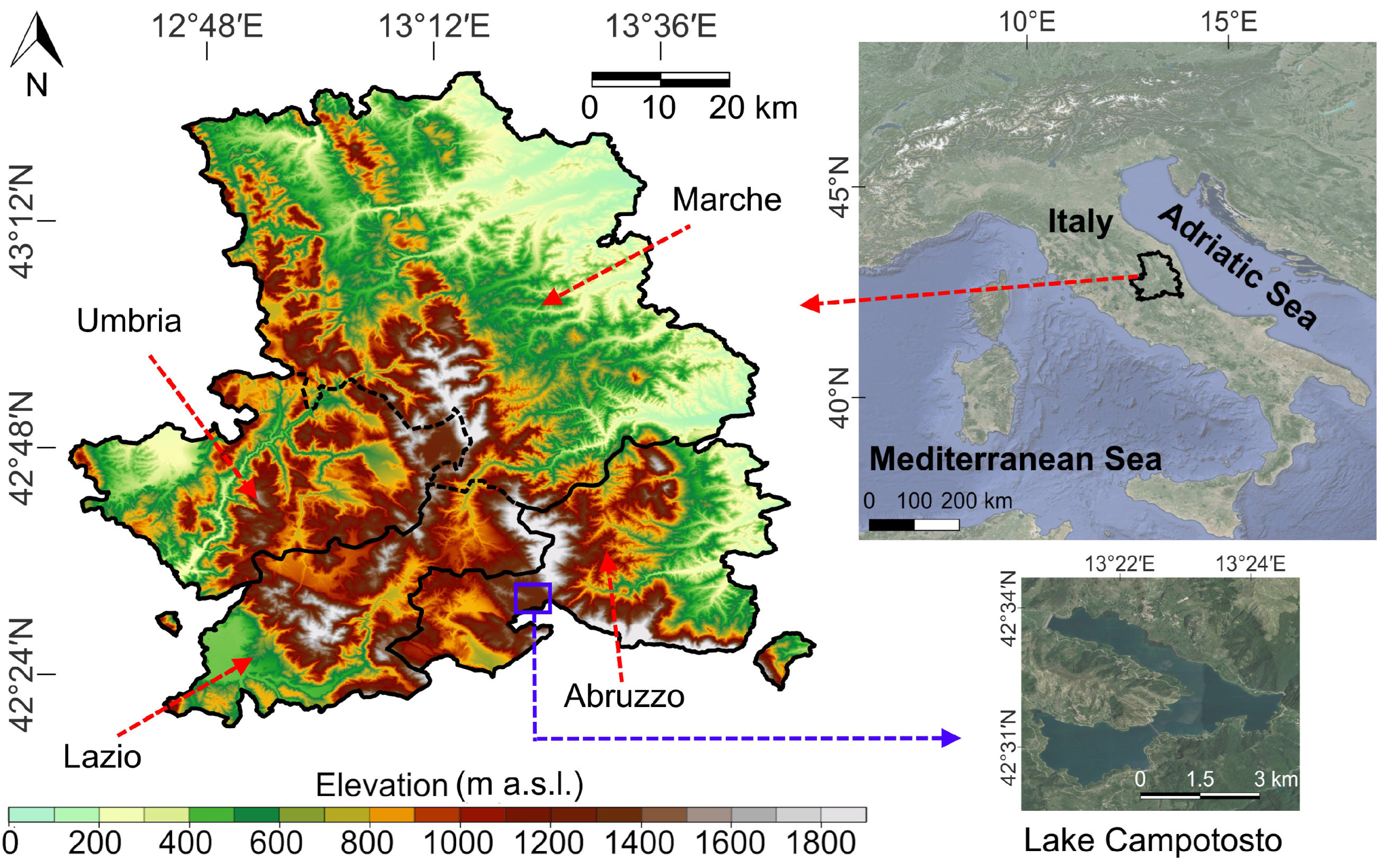
The study region is in Central Italy, which includes parts of Apennines and four Italian administrative regions (Abruzzo, Lazio, Marche, and Umbria) affected by the Amatrice–Norcia–Campotosto seismic sequence (Figure 1). The elevation in Central Italy ranges from zero to a maximum of about 3000 m a.s.l., with the lowest toward the Adriatic Sea and the highest toward its center, i.e., Apennines (Gran Sasso and Monte Vettore). The temperature of this region can be classified as cool (Apennines), sub-continental, and sub-coastal (toward the Adriatic Sea) [31]. The minimum and maximum amounts of monthly accumulated precipitation are roughly in July and November for all four regions, respectively [32]. The median values of the monthly accumulated precipitation in July and November are estimated as 40 mm and 110 mm for Abruzzo, 30 mm and 130 mm for Lazio, 40 mm and 90 mm for Marche, and 30 mm and 110 mm for Umbria, respectively [32] Grasslands, grassy woodlands, and deciduous broadleaf forests are the main land covers of this region [30].
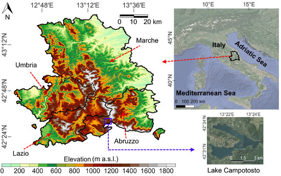
Figure 1.
The study region in Central Italy, including parts of Central Apennines and four administrative regions (Abruzzo, Lazio, Marche, Umbria) with a background DEM–SRTM at 30 m resolution.
2.2. Datasets and Preprocessing
The descriptions of the datasets utilized in this research are listed in Table 1. The Digital Elevation Model (DEM) is from the Shuttle Radar Topography Mission (SRTM Plus) at 30 m resolution, provided by the Jet Propulsion Laboratory (NASA JPL) [33]. The MODIS–LST product is based on the Advanced Spaceborne Thermal Emission and Reflection Radiometer (ASTER) Temperature/Emissivity Separation model, which uses a physics-based algorithm to retrieve both the LST and spectral emissivity simultaneously from the MODIS thermal infrared bands 29, 31, and 32. In this product, an improved water vapor scaling atmospheric correction scheme is utilized to stabilize the retrieval during hot and humid conditions. Daytime and nighttime monthly MODIS–LST images at 1 km resolution from January 2000 to December 2023 can be accessed from the Google Earth Engine (GEE) through the code: ee.ImageCollection(‘MODIS/061/MOD21C3’). The annual MODIS land cover images (MCD12Q1) for the period of 2001–2022 at 500 m are also employed in this research, derived from supervised classifications of MODIS Terra and Aqua reflectance data, and are available from GEE through the code: ee.ImageCollection(‘MODIS/061/MCD12Q1’).

Table 1.
Description of datasets employed in this study.
2.3. Mann–Kendall Trend Test and Sen’s Slope Estimator
The MK is a non-parametric method, named after Mann [34] and Kendall [35], which has been widely used in climate and environmental studies [8]. Let be time series values (). The MK statistic S is defined as
where
When , S is approximately normally distributed with zero mean and standard deviation . The standardized MK statistic Z is given by
When , there is an increasing trend, and vice versa. The estimated trend is statistically significant if , where is the theoretical value for the two-tailed test and is the critical value. Herein, and are selected, corresponding to and confidence intervals, respectively. The MK associated Sen’s slope estimator is a non-parametric estimator defined by [36]:
If , there is an upward trend with a magnitude of ; otherwise, there is a downward trend with magnitude of in the time series. The python package “pyMannKendall”, developed by Hussain and Mahmud [37], is implemented in the present study.
Note that each per-pixel LST time series corresponding to a calendar month has 24 observations, e.g., January 2000, January 2001, …, January 2023. The LST time series utilized in this research have no missing values. Also, each time series derived for each land cover type has 22 observations. For example, a time series value is obtained by counting the number of pixels classified as grasslands for Abruzzo for a calendar year, so a time series of size 22 is derived for the period of 2001–2022 after obtaining such values for each year. The land cover time series utilized in this research are also complete, with no missing values. Note that there is no seasonality from the way the LST time series are constructed, making MK–Sen a reliable approach for testing the trends and estimating the slopes.
2.4. Pearson Correlation Method
The Pearson correlation method is frequently applied to environmental and geoscience applications, among others, for investigating the strength and direction of the relationship between two variables [38,39]. The Pearson r is a normalized value in interval , which shows how far away the data points are from the best fitting line. Pearson r is defined by
where and are the means of variables x and y, respectively. Pearson r values between and indicate a weak correlation. The values between and or and indicate a moderately fuzzy linear dependency, while the values between and or and indicate a strong linear dependency between the variables [3,40]. In this research, the elevation image is downsampled by a median approach and spatially aligned to match with the LST images by the python command: “gdal.ReprojectImage()”. The spatial downsampling of the elevation data using the median approach reduces the effect of potential outliers. For each calendar month and each day or night, the values of the elevation and LST pixels that are spatially aligned are entered into Equation (5) to calculate the r values, i.e., are the LSTs and are their corresponding elevations. Note that no data normalization is required at this stage when applying Equation (5). The flowchart of this work is illustrated in Figure 2.
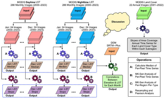
Figure 2.
The flowchart of this work. Each parallelogram represents an image.
3. Results
3.1. Daytime and Nighttime LST Maps for Each Calendar Month
For each calendar month, the median of each per-pixel LST time series is calculated, and the results are illustrated in Figure 3 and Figure 4 for day and night, respectively. The value of each pixel in each map is the median of an LST time series of size 24 for the period of 2000–2023. Note that the spatial resolution of each pixel is 1 km, as directly provided by GEE using ee.ImageCollection(‘MODIS/061/MOD21C3’)—the original spatial resolution of the product is 0.05° × 0.05°.
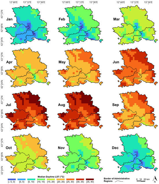
Figure 3.
LST median daytime spatial maps for the calendar months.
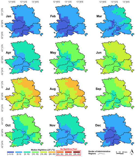
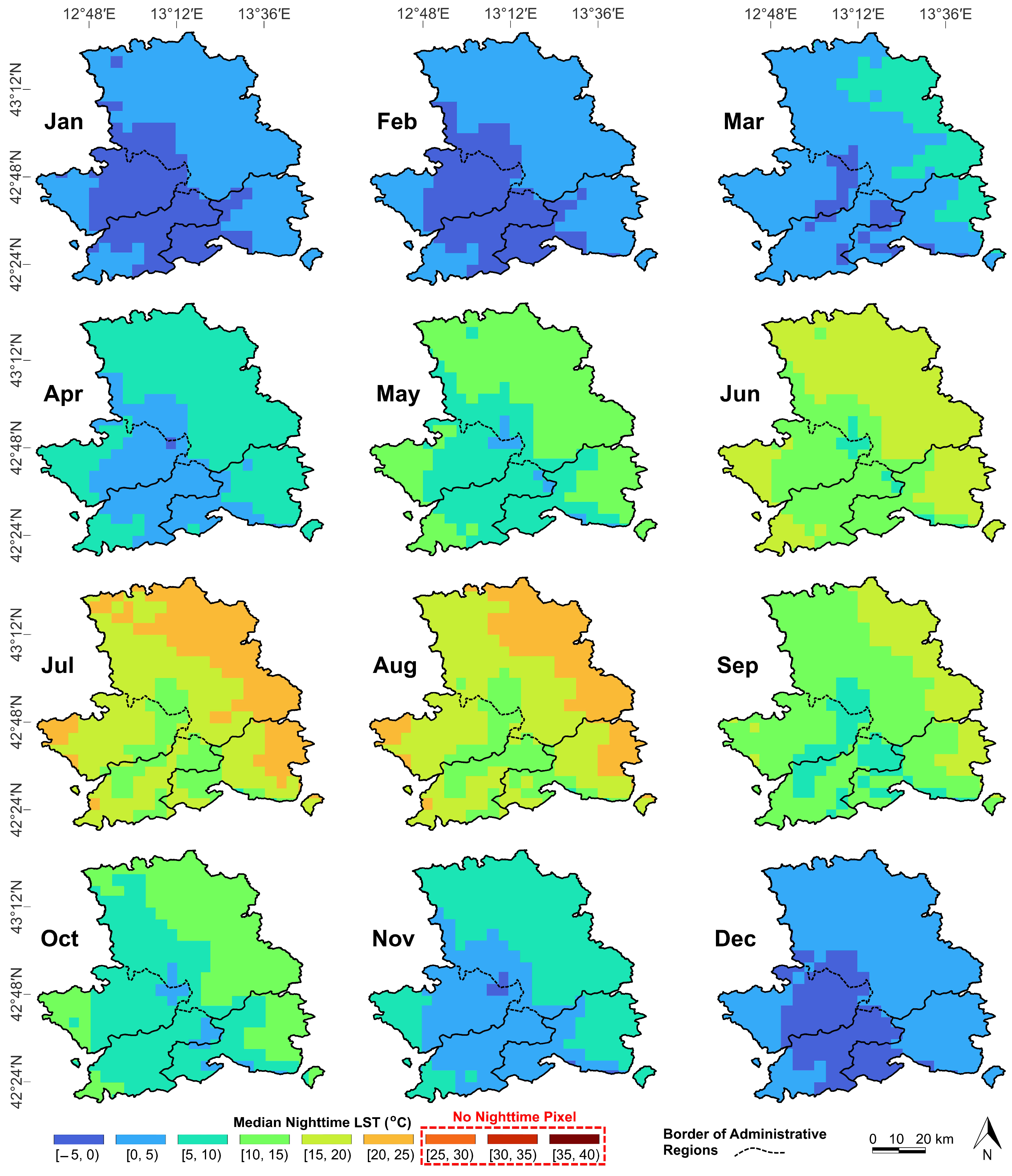
Figure 4.
LST median nighttime spatial maps for the calendar months.
From the figures, a negative daytime and nighttime LST during the winter (December, January and February) can be observed in the high altitude areas of the Apennines. The median nighttime LST does not exceed 25 °C in all twelve months (see Figure 4). On the other hand, the median daytime LST reaches 40 °C during the summer, mainly in Marche near the coast with low altitudes (see Figure 3).
3.2. Daytime and Nighttime LST Sen’s Slope Maps for Each Calendar Month
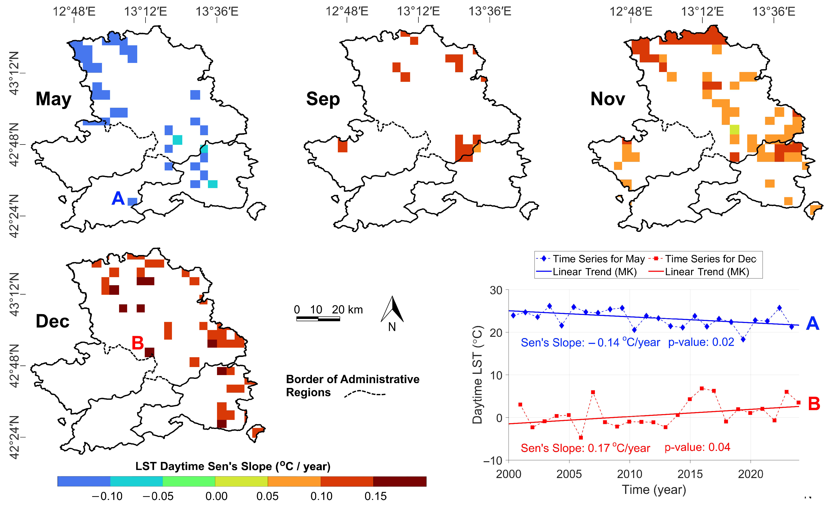
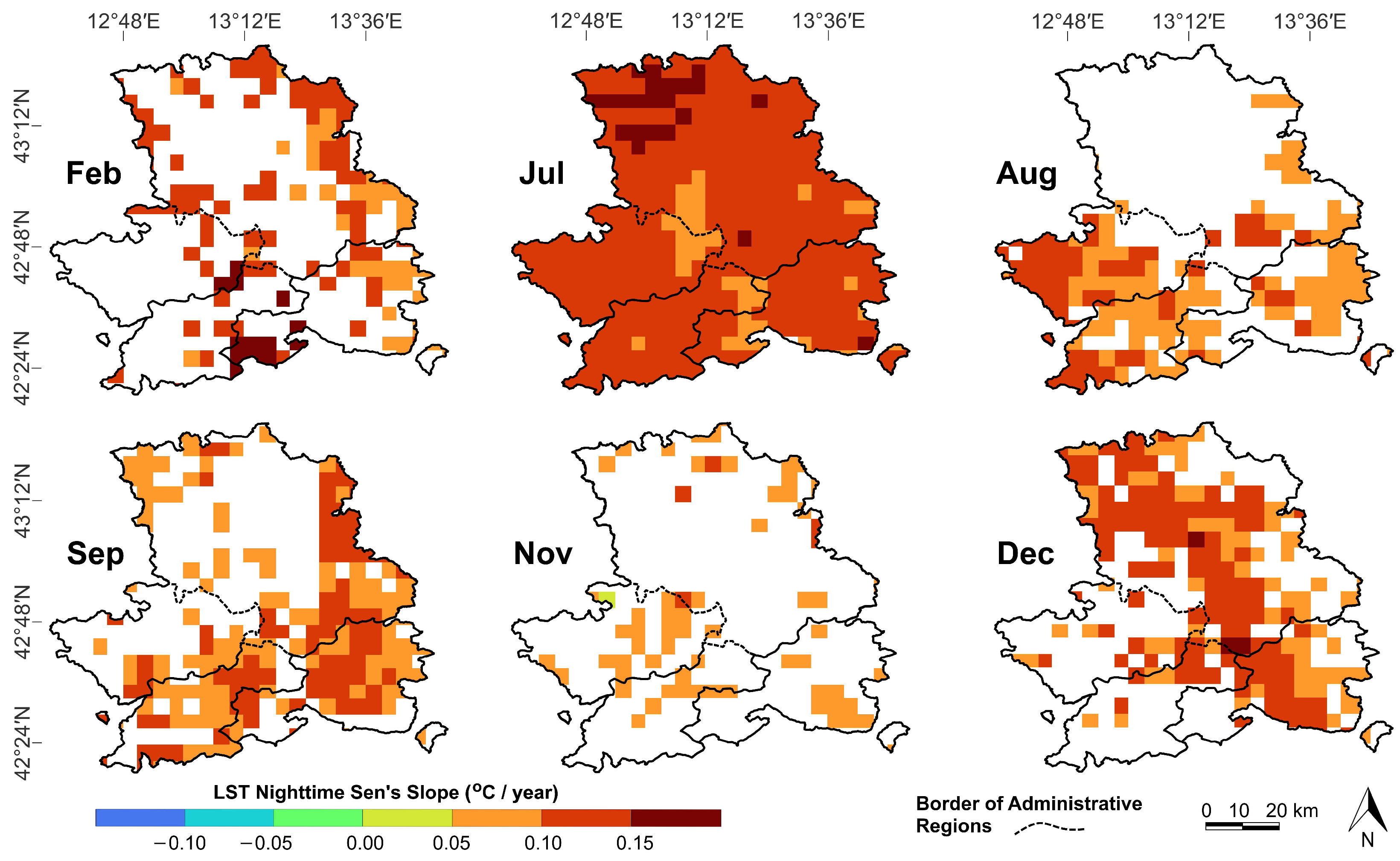
For each calendar month, MK–Sen is applied to each per-pixel time series of size 24. For the daytime imagery, it is found that only May, September, November, and December have statistically significant cooling/warming trends. Figure 5 shows that, since 2000, May has been cooling, while September, November, and December have been warming. For a better understanding and visualization of the estimated MK–Sen linear trends, two per-pixel time series were selected in May and December (labeled as A and B, respectively), and their linear trend results are displayed in the bottom right of Figure 5. For the nighttime images, only six months (February, July, August, September, November, and December) show statistically significant slopes at a 95% confidence level, where the regions have just been warming during these six months, i.e., all calendar months show no nighttime cooling trend (see Figure 6). Interestingly, the whole study region in July has been significantly warming during the night.

Figure 5.
LST daytime spatial maps of Sen’s slopes for the calendar months at a 95% confidence level.

Figure 6.
LST nighttime spatial maps of Sen’s slopes for the calendar months at a 95% confidence level.
3.3. Land Cover Change Results
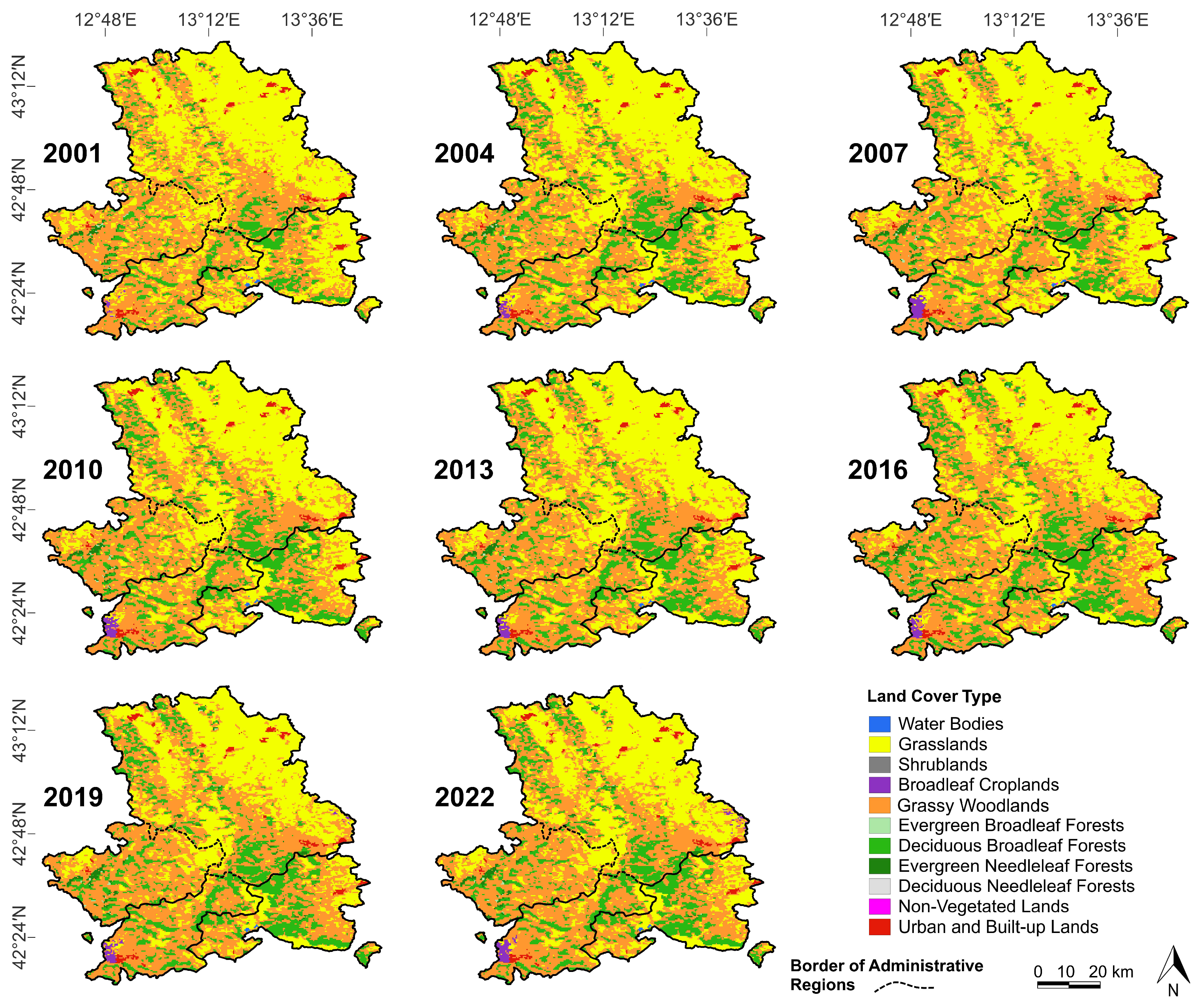
To visualize how the land cover types have been changing in the study region, the MODIS annual land cover images for the years 2001, 2004, 2007, 2010, 2013, 2016, 2019, and 2022 are first illustrated in Figure 7.
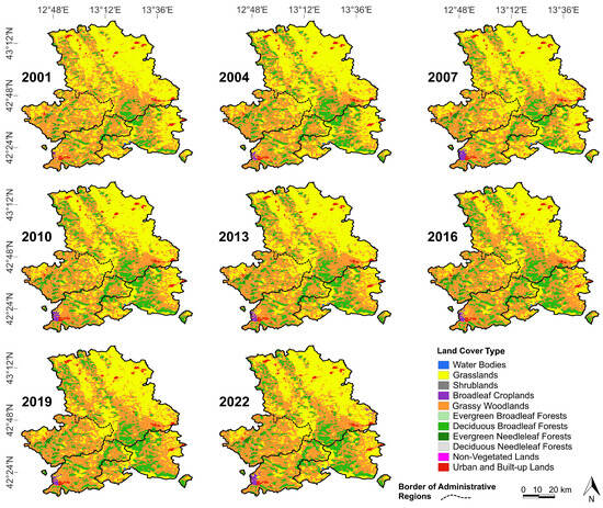
Figure 7.
The MODIS land cover maps with 11 classes at 500 m spatial resolution for the study region.
More than 90% of the subregions are covered by only three land cover types, namely grasslands, grassy woodlands, and deciduous broadleaf forests. According to the MODIS collection 6.1 (C61) land cover type product user guide, grasslands are areas covered by herbaceous annuals (<2 m height), including cereal croplands, while grassy woodlands are areas (pixels of 500 m resolution) with a tree coverage (>2 m height) of between 10% and 60%. Deciduous broadleaf forests are areas dominated by deciduous broadleaf trees (>2 m height) with more than 60% tree coverage. The urban and built-up lands within the study region remain unchanged, except for an expansion of 1 km2 (four pixels only) in Marche from 2005 to 2008.
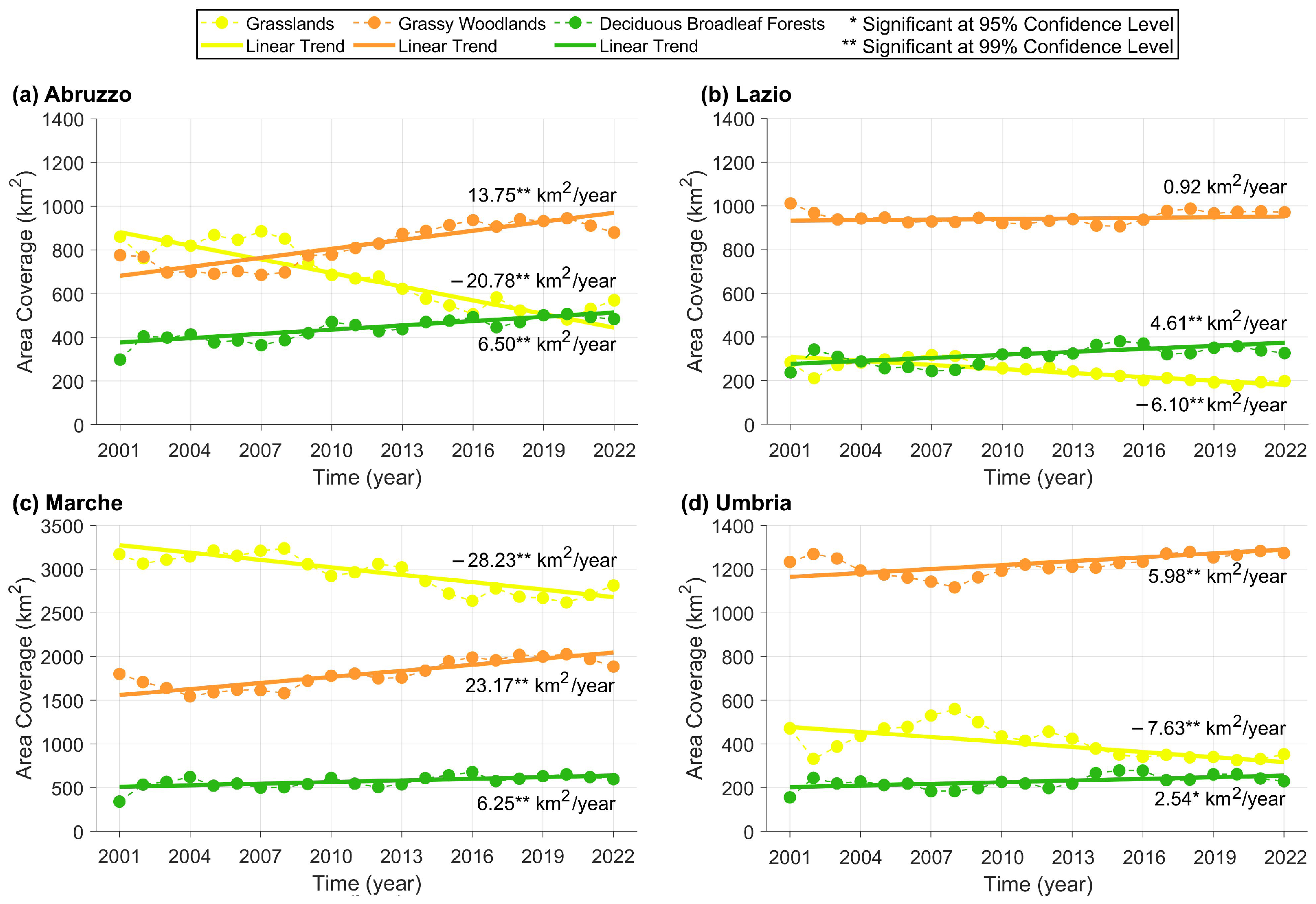
The land cover change is estimated by MK–Sen for the three main land cover types, and the results are illustrated in Figure 8. Each annual time series, shown in Figure 8, is obtained by counting the number of pixels classified as a particular land cover type within each subregion for each calendar year, multiplied by 0.25 km2 (the approximate area of each pixel). The size of each time series is 22, i.e., one observation for each year from 2001 to 2023. It is clear from Figure 8 that grasslands have been decreasing, while woodlands and forests have been significantly expanding within each subregion. In fact, the grasslands have been replaced mainly by woodlands and forests. Afforestation or forest expansion in the Central Apennines, partially due to anthropogenic activities, has been occurring in recent decades, and has been studied in the literature [41,42].
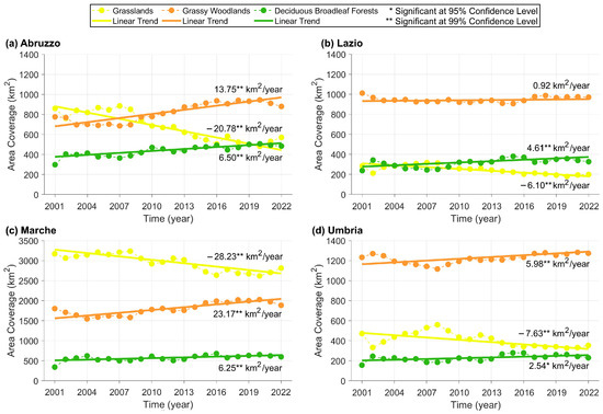
Figure 8.
The MK–Sen results of the annual land cover time series for each subregion at a 95% confidence level.
Table 2 shows another representation of MK–Sen analysis. The numbers in Table 2 are the Sen’s slopes with the unit of percentage area coverage per year, where the percentage area coverage of each land cover type within each subregion is obtained from dividing the number of pixels for each land cover type by the total number of pixels in that subregion, multiplied by 100. Note that the Sen’s slopes written on the graphs in Figure 8 are expressed in terms of km2/year.
Table 2.
The MK–Sen trend results in (%)/year for the four subregions.
3.4. Correlation between LST and Elevation
To investigate the potential factors influencing LST variations across the study region, correlation analysis between LST and elevation is performed. Table 3 shows the Pearson r values between the elevation and the daytime (nighttime) median LSTs during 2000–2023 for each calendar month. It can be seen that a strong negative correlation exists between the LST and the elevation, more significantly during winter for daytime LST and during summer for nighttime LST.
Table 3.
Pearson r values between the elevation and LST for the study region.
4. Discussion
4.1. Relationships between LST and Land Cover
Cooling and warming trends in LST are mainly driven by evapotranspiration and albedo, and heavily influenced by precipitation [15,43]. The nighttime warming trend in the study region can be explained by the woodland and forest expansions. Since trees, particularly deciduous broadleaf trees, can absorb heat during the day, they release it slowly during the night, causing a warmer microclimate around them [43]. Furthermore, trees can impede the wind from the ground to the treetops, reducing the cooling effect of wind chill, which can potentially explain the nighttime warming effect, as observed in Figure 6. During the winter, the trees can have a warming effect on surface, and they act as a warm blanket, which can also explain the daytime warming trend in Marche and Abruzzo, which have the highest rates of forest expansion (see Figure 5 and Figure 8). As also pointed out by Li et al. [43], during the growing seasons in early summer (e.g., May), daytime cooling usually dominates forests and due to weaker nighttime warming, the net daily cooling effect is observed during May across the Apennines (see Figure 5, and Figure A.5 in [3]). The overall LST trends for the study region since 2000 are estimated as approximately 0.01 °C/year for the daytime, 0.03 °C/year for the nighttime, and 0.02 °C/year daily (see Table A.2 in [3]).
4.2. Relationships between LST and Elevation
The correlation between the LST and the elevation has been studied by many researchers. For example, Elijah et al. [44] found that land cover explained the LST variations across their study region in Nigeria, but they did not observe any significant correlations between elevation and LST due to a relatively low elevation range in their region. Peng et al. [45] observed a significant linear relationship between the LST and the elevation in Hangzhou, China. They also showed that the LST decreases with an increasing elevation in winter in their region. The results of the current study indicate that the elevation and the land cover can explain the LST variations to a great extent in Central Italy. Table 3 shows that November, December, January, and February have significant negative correlations () between the daytime LST and the elevation, while May, June, July, August, and September have significant negative correlations () between the nighttime LST and the elevation. The negative correlation between the LST and the elevation agrees with the fact that air molecules are more spread out at higher altitudes. In other words, the air pressure decreases as the elevation increases, reducing the air temperature and LST, where the reduction amount depends on the moisture condition [46].
4.3. Insights into Natural and Geological Hazards
Gradual warming, woodland and forest expansions, and dry spells can potentially increase the severity and occurrences of wildfires in the study region, and pose a significant risk to the biodiversity, greenhouse gas emissions, and infrastructure, as well as increasing the risk of post-fire shallow landslides and debris flows [47]. Thus, utilizing machine learning and statistical modeling to creating wildfire susceptibility maps and risk forecasting in this region becomes crucial [48,49].
The significant nighttime warming trend observed in the study region may change the soil and rockwall erosion rates. It can potentially alter the groundwater level, trigger landslides, and amplify high-magnitude rockfalls through water advection associated with snow cover and ice melting in rock discontinuities and joints [50,51,52,53]. Gradual declining of the precipitation in Abruzzo, Lazio, Marche, and Umbria is observed since 2000, with extreme precipitation events in recent years, particularly in Lazio (see Figure 3 in [32]). Extreme precipitation events followed by dry spells trigger landslides and reactivates slow-moving landslides—such extreme events are likely to continue in the upcoming years [54,55].
In the study region, there are not many large-sized water bodies to be studied. There is only an artificial lake, called Lake Campotosto, which is a migratory site for many animal species. Lake Campotosto is a protected area in the province of L’Aquila in Abruzzo, with an area of ≈14 km2, a depth of 30–35 m, and an altitude of ≈1313 m a.s.l. [56], highlighted in Figure 1. The MK–Sen analysis on the MODIS land cover product reveals that the water surface extent may have decreased by a rate of 0.075 km2/year or 0.004 (%)/year at a 99% confidence level since 2001. Although the trend results on the limited water bodies may provide an insight on the impact of climate change and human activity, the spatial resolution of MODIS land cover (500 m) is too low to provide a concrete solution for the water surface dynamics of the lake. A more in-depth analysis would be to utilize higher resolution satellite imagery, such as Landsat (30 m), Sentinel (10 m), and PlanetScope (3 m), which allows for more accurate water surface dynamic monitoring [57,58].
Santis et al. [59] investigated the impact of climate change on small-to-medium Italian lakes in Central Italy through moderate resolution satellite data, including Landsat and Sentinel. They showed that the surface temperature of the lakes increased by ≈0.11 °C/year since 2000. Figure 6 also shows that the nighttime LST has risen in February, July, September and December, particularly by more than 0.15 °C/year in February. Antonielli et al. [56] conducted a multi-hazard research on this lake, and pointed out that the region may be impacted by a complex earthquake-induced chain of geologic hazards, such as the seismic shaking, earthquake-triggered landslides, and surface faulting of the Gorzano Mt. Fault. The observed nighttime warming trend and a gradual reduction in the water surface extent of this lake may provide further insight on multi-risk and multi-hazard assessment, as discussed in [60,61].
4.4. Limitations and Future Direction
The aim of this research is to provide a broad view of the climate and land cover variations in Central Italy, focusing on the monthly daytime and nighttime surface temperature trends. The MODIS spatial resolution is relatively lower than the resolution of other thermal sensors on board satellites, such as Landsat and Sentinel. Combining the data acquired from these sensors can provide a more detailed analysis. The methods applied here are also simple and easy to understand. More sophisticated data analytics techniques, such as wavelets, machine learning, and deep learning models, can be utilized to better aid understanding of the interconnections between climate, elevation, and land cover.
5. Conclusions
In this study, the MODIS products are employed to estimate linear trends in the daytime and nighttime LST (2000–2023) and land cover (2001–2022) time series in Central Italy. The non-parametric Mann–Kendall trend model, and its associated Sen’s slope, are applied to estimate the linear trends. Possible relationships between the LST and land cover are discussed, and the Pearson correlation between the LST and elevation is also estimated. The main results are summarized below:
- Statistically significant warming trends are observed during the night for February, July, August, September, November, and December.
- Statistically significant warming trends are observed during the day for September, November, and December, mainly in Marche and Abruzzo, which are closer to the coast.
- The elevation is found to be negatively correlated with the LST, more strongly for daytime during winter and nighttime during summer.
- Woodlands and forest expansion explains the nighttime warming trends that are more dominant than the daytime trends in the region.
- Potential geohazards due to recent LST and land cover changes are also discussed.
It is hoped that the presented results could be useful for various purposes, including landslide and wildfire susceptibility analysis. Future work would focus on integrating higher resolution satellite data, as well as more advanced data analytics models to provide a more in-depth analysis for Central Italy.
Author Contributions
Conceptualization, E.G., P.M., F.B. and G.S.M.; Methodology, E.G.; Formal analysis, E.G.; Visualization, E.G.; Writing—original draft, E.G.; Writing—review and editing, P.M., F.B. and G.S.M. All authors have read and agreed to the published version of the manuscript.
Funding
This research was financially supported by the CERI research centre at Sapienza University of Rome and ABDAC project: (000158_2021_ABDAC_Scarascia).
Data Availability Statement
The MODIS LST and land cover images employed in this research are freely available and can be downloaded at https://doi.org/10.5067/MODIS/MOD21C3.061 (accessed on 12 May 2024) and https://doi.org/10.5067/MODIS/MCD12Q1.061 (accessed on 12 May 2024), respectively.
Acknowledgments
The authors thank NASA scientists and personnel for providing the MODIS products utilized in this research.
Conflicts of Interest
The authors are empolyed by NHAZCA s.r.l. The authors declare no conflicts of interest.
References
- Li, Z.L.; Wu, H.; Duan, S.B.; Zhao, W.; Ren, H.; Liu, X. Satellite remote sensing of global land surface temperature: Definition, methods, products, and applications. Rev. Geophys. 2023, 61, e2022RG000777. [Google Scholar] [CrossRef]
- Bindajam, A.A.; Mallick, J.; AlQadhi, S.; Singh, C.K.; Hang, H.T. Impacts of Vegetation and Topography on Land Surface Temperature Variability over the Semi-Arid Mountain Cities of Saudi Arabia. Atmosphere 2020, 11, 762. [Google Scholar] [CrossRef]
- Ghaderpour, E.; Mazzanti, P.; Scarascia Mugnozza, G.; Bozzano, F. Coherency and phase delay analyses between land cover and climate across Italy via the least-squares wavelet software. Int. J. Appl. Earth Obs. Geoinf. 2023, 118, 103241. [Google Scholar] [CrossRef]
- Cammalleri, C.; Vogt, J. On the Role of Land Surface Temperature as Proxy of Soil Moisture Status for Drought Monitoring in Europe. Remote Sens. 2015, 7, 16849–16864. [Google Scholar] [CrossRef]
- Loche, M.; Scaringi, G.; Yunus, A.P.; Catani, F.; Tanyaş, H.; Frodella, W.; Fan, X.; Lombardo, L. Surface temperature controls the pattern of post-earthquake landslide activity. Sci. Rep. 2022, 12, 988. [Google Scholar] [CrossRef]
- Khamidov, M.; Ishchanov, J.; Hamidov, A.; Shermatov, E.; Gafurov, Z. Impact of Soil Surface Temperature on Changes in the Groundwater Level. Water 2023, 15, 3865. [Google Scholar] [CrossRef]
- Yu, P.; Zhao, T.; Shi, J.; Ran, Y.; Jia, L.; Ji, D.; Xue, H. Global spatiotemporally continuous MODIS land surface temperature dataset. Sci. Data 2022, 9, 143. [Google Scholar] [CrossRef]
- Ahmed, M.R.; Ghaderpour, E.; Gupta, A.; Dewan, A.; Hassan, Q.K. Opportunities and Challenges of Spaceborne Sensors in Delineating Land Surface Temperature Trends: A Review. IEEE Sens. J. 2023, 23, 6460–6472. [Google Scholar] [CrossRef]
- Pan, X.; Wang, Z.; Liu, S.; Yang, Z.; Guluzade, R.; Liu, Y.; Yuan, J.; Yang, Y. The impact of clear-sky biases of land surface temperature on monthly evapotranspiration estimation. Int. J. Appl. Earth Obs. Geoinf. 2024, 129, 103811. [Google Scholar] [CrossRef]
- Wan, Z.; Zhang, Y.; Zhang, Q.; Li, Z.l. Validation of the land-surface temperature products retrieved from Terra Moderate Resolution Imaging Spectroradiometer data. Remote Sens. Environ. 2002, 83, 163–180. [Google Scholar] [CrossRef]
- Zhao, B.; Mao, K.; Cai, Y.; Shi, J.; Li, Z.; Qin, Z.; Meng, X.; Shen, X.; Guo, Z. A combined Terra and Aqua MODIS land surface temperature and meteorological station data product for China from 2003 to 2017. Earth Syst. Sci. Data 2020, 12, 2555–2577. [Google Scholar] [CrossRef]
- Eleftheriou, D.; Kiachidis, K.; Kalmintzis, G.; Kalea, A.; Bantasis, C.; Koumadoraki, P.; Spathara, M.E.; Tsolaki, A.; Tzampazidou, M.I.; Gemitzi, A. Determination of annual and seasonal daytime and nighttime trends of MODIS LST over Greece—Climate change implications. Sci. Total Environ. 2018, 616–617, 937–947. [Google Scholar] [CrossRef]
- Waring, A.M.; Ghent, D.; Perry, M.; Anand, J.S.; Veal, K.L.; Remedios, J. Regional climate trend analyses for Aqua MODIS land surface temperatures. Int. J. Remote Sens. 2023, 44, 4989–5032. [Google Scholar] [CrossRef]
- Siddiqui, A.; Kushwaha, G.; Nikam, B.; Srivastav, S.; Shelar, A.; Kumar, P. Analysing the day/night seasonal and annual changes and trends in land surface temperature and surface urban heat island intensity (SUHII) for Indian cities. Sustain. Cities Soc. 2021, 75, 103374. [Google Scholar] [CrossRef]
- Shawky, M.; Razu Ahmed, M.; Ghaderpour, E.; Gupta, A.; Achari, G.; Dewan, A.; Hassan, Q.K. Remote sensing-derived land surface temperature trends over South Asia. Ecol. Inform. 2023, 74, 101969. [Google Scholar] [CrossRef]
- Gao, H.; Jin, J. Analysis of Water Yield Changes from 1981 to 2018 Using an Improved Mann-Kendall Test. Remote Sens. 2022, 14, 2009. [Google Scholar] [CrossRef]
- Wang, F.; Shao, W.; Yu, H.; Kan, G.; He, X.; Zhang, D.; Ren, M.; Wang, G. Re-evaluation of the Power of the Mann-Kendall Test for Detecting Monotonic Trends in Hydrometeorological Time Series. Front. Earth Sci. 2020, 8, 14. [Google Scholar] [CrossRef]
- Marzocchi, W.; Taroni, M.; Falcone, G. Earthquake forecasting during the complex Amatrice-Norcia seismic sequence. Sci. Adv. 2017, 3, e1701239. [Google Scholar] [CrossRef]
- Sebastiani, G.; Govoni, A.; Pizzino, L. Aftershock patterns in recent central Apennines sequences. J. Geophys. Res. Solid Earth 2019, 124, 3881–3897. [Google Scholar] [CrossRef]
- Sisti, R.; Di Ludovico, M.; Borri, A.; Prota, A. Damage assessment and the effectiveness of prevention: The response of ordinary unreinforced masonry buildings in Norcia during the Central Italy 2016–2017 seismic sequence. Bull. Earthq. Eng. 2019, 17, 5609–5629. [Google Scholar] [CrossRef]
- Pagliacci, F.; Luciani, C.; Russo, M.; Esposito, F.; Habluetzel, A. The socioeconomic impact of seismic events on animal breeding. A questionnaire-based survey from central Italy. Int. J. Disaster Risk Reduct. 2021, 56, 102124. [Google Scholar] [CrossRef]
- Bozzano, F.; Carabella, C.; De Pari, P.; Discenza, M.; Fantucci, R.; Mazzanti, P.; Miccadei, E.; Rocca, A.; Romano, S.; Sciarra, N. Geological and geomorphological analysis of a complex landslides system: The case of San Martino sulla Marruccina (Abruzzo, Central Italy). J. Maps 2020, 16, 126–136. [Google Scholar] [CrossRef]
- Carboni, F.; Porreca, M.; Valerio, E.; Mariarosaria, M.; De Luca, C.; Azzaro, S.; Ercoli, M.; Barchi, M.R. Surface ruptures and off-fault deformation of the October 2016 central Italy earthquakes from DInSAR data. Sci. Rep. 2022, 12, 3172. [Google Scholar] [CrossRef]
- Donnini, M.; Santangelo, M.; Gariano, S.; Bucci, F.; Peruccacci, S.; Alvioli, M.; Althuwaynee, O.; Ardizzone, F.; Bianchi, C.; Bornaetxea, T.; et al. Landslides triggered by an extraordinary rainfall event in Central Italy on 15 September 2022. Landslides 2023, 20, 2199–2211. [Google Scholar] [CrossRef]
- Kamps, M.; Bouten, W.; Seijmonsbergen, A.C. LiDAR and Orthophoto Synergy to optimize Object-Based Landscape Change: Analysis of an Active Landslide. Remote Sens. 2017, 9, 805. [Google Scholar] [CrossRef]
- Liu, B.; Song, W.; Meng, Z.; Liu, X. Review of Land Use Change Detection–A Method Combining Machine Learning and Bibliometric Analysis. Land 2023, 12, 1050. [Google Scholar] [CrossRef]
- Pacheco Quevedo, R.; Velastegui-Montoya, A.; Montalván-Burbano, N.; Morante-Carballo, F.; Korup, O.; Daleles Rennó, C. Land use and land cover as a conditioning factor in landslide susceptibility: A literature review. Landslides 2023, 20, 967–982. [Google Scholar] [CrossRef]
- Vlassova, L.; Pérez-Cabello, F.; Mimbrero, M.; Llovería, R.; García-Martín, A. Analysis of the Relationship between Land Surface Temperature and Wildfire Severity in a Series of Landsat Images. Remote Sens. 2014, 6, 6136–6162. [Google Scholar] [CrossRef]
- Zhao, B.; Dai, Q.; Zhuo, L.; Zhu, S.; Shen, Q.; Han, D. Assessing the potential of different satellite soil moisture products in landslide hazard assessment. Remote Sens. Environ. 2021, 264, 112583. [Google Scholar] [CrossRef]
- Malandra, F.; Vitali, A.; Urbinati, C.; Garbarino, M. 70 Years of Land Use/Land Cover Changes in the Apennines (Italy): A Meta-Analysis. Forests 2018, 9, 551. [Google Scholar] [CrossRef]
- Fratianni, S.; Acquaotta, F. The Climate of Italy. In Landscapes and Landforms of Italy; Soldati, M., Marchetti, M., Eds.; Springer International Publishing: Cham, Switzerland, 2017; pp. 29–38. [Google Scholar] [CrossRef]
- Ghaderpour, E.; Dadkhah, H.; Dabiri, H.; Bozzano, F.; Scarascia Mugnozza, G.; Mazzanti, P. Precipitation Time Series Analysis and Forecasting for Italian Regions. Eng. Proc. 2023, 39, 23. [Google Scholar] [CrossRef]
- Farr, T.G.; Rosen, P.A.; Caro, E.; Crippen, R.; Duren, R.; Hensley, S.; Kobrick, M.; Paller, M.; Rodriguez, E.; Roth, L.; et al. The shuttle radar topography mission. Rev. Geophys. 2007, 45, RG2004. [Google Scholar] [CrossRef]
- Mann, H.B. Nonparametric tests against trend. Econom. J. Econom. Soc. 1945, 13, 245–259. [Google Scholar] [CrossRef]
- Kendall, M.G. Rank Correlation Methods; Griffin: London, UK, 1948. [Google Scholar]
- Sen, P.K. Estimates of the Regression Coefficient based on Kendall’s Tau. J. Am. Stat. Assoc. 1968, 63, 1379–1389. [Google Scholar] [CrossRef]
- Hussain, M.; Mahmud, I. pyMannKendall: A python package for non parametric Mann Kendall family of trend tests. J. Open Source Softw. 2019, 4, 1556. [Google Scholar] [CrossRef]
- Liu, Y.; Shana, F.; Yue, H.; Wanga, X.; Fan, Y. Global analysis of the correlation and propagation among meteorological, agricultural, surface water, and groundwater droughts. J. Environ. Manag. 2023, 333, 117460. [Google Scholar] [CrossRef]
- Araujo, M.; Rufino, I.; Silva, F.; Brito, H.; Santos, J. The Relationship between Climate, Agriculture and Land Cover in Matopiba, Brazil (1985–2020). Sustainability 2024, 16, 2670. [Google Scholar] [CrossRef]
- Ratner, B. The correlation coefficient: Its values range between +1/–1, or do they? J. Target. Meas. Anal. Mark. 2009, 17, 139–142. [Google Scholar] [CrossRef]
- Vacchiano, G.; Garbarino, M.; Lingua, E.; Motta, R. Forest dynamics and disturbance regimes in the Italian Apennines. For. Ecol. Manag. 2017, 388, 57–66. [Google Scholar] [CrossRef]
- Cavalli, A.; Francini, S.; Cecili, G.; Cocozza, C.; Congedo, L.; Falanga, V.; Spadoni, G.; Maesano, M.; Munafo, M.; Chirici, G.; et al. Afforestation monitoring through automatic analysis of 36-years Landsat Best Available Composites. iForest Biogeosci. For. 2022, 15, 220–228. [Google Scholar] [CrossRef]
- Li, Y.; Zhao, M.; Motesharrei, S.; Mu, Q.; Kalnay, E.; Li, S. Local cooling and warming effects of forests based on satellite observations. Nat. Commun. 2015, 6, 6603. [Google Scholar] [CrossRef]
- Njoku, E.A.; Tenenbaum, D.E. Quantitative assessment of the relationship between land use/land cover (LULC), topographic elevation and land surface temperature (LST) in Ilorin, Nigeria. Remote Sens. Appl. Soc. Environ. 2022, 27, 100780. [Google Scholar] [CrossRef]
- Peng, X.; Wu, W.; Zheng, Y.; Sun, J.; Hu, T.; Wang, P. Correlation analysis of land surface temperature and topographic elements in Hangzhou, China. Sci. Rep. 2020, 10, 10451. [Google Scholar] [CrossRef]
- Phan, T.; Kappas, M.; Tran, T. Land Surface Temperature Variation Due to Changes in Elevation in Northwest Vietnam. Climate 2018, 6, 28. [Google Scholar] [CrossRef]
- Culler, E.S.; Livneh, B.; Rajagopalan, B.; Tiampo, K.F. A data-driven evaluation of post-fire landslide susceptibility. Nat. Hazards Earth Syst. Sci. 2023, 23, 1631–1652. [Google Scholar] [CrossRef]
- Salavati, G.; Saniei, E.; Ghaderpour, E.; Hassan, Q. Wildfire Risk Forecasting Using Weights of Evidence and Statistical Index Models. Sustainability 2022, 14, 3881. [Google Scholar] [CrossRef]
- Trucchia, A.; Meschi, G.; Fiorucci, P.; Gollini, A.; Negro, D. Defining Wildfire Susceptibility Maps in Italy for Understanding Seasonal Wildfire Regimes at the National Level. Fire 2022, 5, 30. [Google Scholar] [CrossRef]
- Mazzanti, P.; Schilirò, L.; Martino, S.; Antonielli, B.; Brizi, E.; Brunetti, A.; Margottini, C.; Scarascia Mugnozza, G. The Contribution of Terrestrial Laser Scanning to the Analysis of Cliff Slope Stability in Sugano (Central Italy). Remote Sens. 2018, 10, 1475. [Google Scholar] [CrossRef]
- Martino, S.; Cercato, M.; Della Seta, M.; Esposito, C.; Hailemikael, S.; Iannucci, R.; Martini, G.; Paciello, A.; Scarascia Mugnozza, G.; Seneca, D.; et al. Relevance of rock slope deformations in local seismic response and microzonation: Insights from the Accumoli case-study (central Apennines, Italy). Eng. Geol. 2020, 266, 105427. [Google Scholar] [CrossRef]
- Birien, T.; Gauthier, F. Assessing the relationship between weather conditions and rockfall using terrestrial laser scanning to improve risk management. Nat. Hazards Earth Syst. Sci. 2023, 23, 343–360. [Google Scholar] [CrossRef]
- Grechi, G.; D’Angiò, D.; Martino, S. Analysis of Thermally Induced Strain Effects on a Jointed Rock Mass through Microseismic Monitoring at the Acuto Field Laboratory (Italy). Appl. Sci. 2023, 13, 2489. [Google Scholar] [CrossRef]
- Tichavský, R.; Ballesteros-Cánovas, J.A.; Šilhán, K.; Tolasz, R.; Stoffel, M. Dry Spells and Extreme Precipitation are The Main Trigger of Landslides in Central Europe. Sci. Rep. 2019, 9, 14560. [Google Scholar] [CrossRef]
- Ghaderpour, E.; Antonielli, B.; Bozzano, F.; Scarascia Mugnozza, G.; Mazzanti, P. A fast and robust method for detecting trend turning points in InSAR displacement time series. Comput. Geosci. 2024, 185, 105546. [Google Scholar] [CrossRef]
- Antonielli, B.; Bozzano, F.; Fiorucci, M.; Hailemikael, S.; Iannucci, R.; Martino, S.; Rivellino, S.; Scarascia Mugnozza, G. Engineering-Geological Features Supporting a Seismic-Driven Multi-Hazard Scenario in the Lake Campotosto Area (L’Aquila, Italy). Geosciences 2021, 11, 107. [Google Scholar] [CrossRef]
- Yang, X.; Chen, Y.; Wang, J. Combined use of Sentinel-2 and Landsat 8 to monitor water surface area dynamics using Google Earth Engine. Remote Sens. Lett. 2020, 11, 687–696. [Google Scholar] [CrossRef]
- Acharki, S. PlanetScope contributions compared to Sentinel-2, and Landsat-8 for LULC mapping. Remote Sens. Appl. Soc. Environ. 2022, 27, 100774. [Google Scholar] [CrossRef]
- De Santis, D.; Del Frate, F.; Schiavon, G. Analysis of Climate Change Effects on Surface Temperature in Central-Italy Lakes Using Satellite Data Time-Series. Remote Sens. 2022, 14, 117. [Google Scholar] [CrossRef]
- Verdecchia, A.; Deng, K.; Harrington, R.M.; Liu, Y. How Might Draining Lake Campotosto Affect Stress and Seismicity on the Monte Gorzano Normal Fault, Central Italy? Agu Fall Meet. Abstr. 2017, 2017, NH33D-03. [Google Scholar]
- Verdecchia, A.; Deng, K.; Harrington, R.; Liu, Y. The effect of lake drainage on active faults: Two examples from central Italy. In Proceedings of the 20th EGU General Assembly, EGU2018, Vienna, Austria, 4–13 April 2018; Available online: https://ui.adsabs.harvard.edu/abs/2018EGUGA..20.9277V (accessed on 12 May 2024).


Disclaimer/Publisher’s Note: The statements, opinions and data contained in all publications are solely those of the individual author(s) and contributor(s) and not of MDPI and/or the editor(s). MDPI and/or the editor(s) disclaim responsibility for any injury to people or property resulting from any ideas, methods, instructions or products referred to in the content. |
© 2024 by the authors. Licensee MDPI, Basel, Switzerland. This article is an open access article distributed under the terms and conditions of the Creative Commons Attribution (CC BY) license (https://creativecommons.org/licenses/by/4.0/).