Calculation of the Optimal Scale of Urban Green Space for Alleviating Surface Urban Heat Islands: A Case Study of Xi’an, China

Abstract

Research has demonstrated that urban green spaces play a crucial role in mitigating the severe urban heat island (UHI) effect. However, existing studies often suffer from limitations such as the neglect of the cooling effect of water bodies within the green spaces and incomplete considerations of the overall cooling effect. These limitations may lead to inaccuracies in the research findings. Therefore, the present study takes the city of Xi’an as a case study to explore the optimal green space size for achieving efficient cooling. The results indicate that (i) urban green spaces exhibit robust cooling effects, with variations observed among the various types; (ii) for community parks without water, and for street gardens, the optimal areas of these green spaces are 3.44 and 0.83 hectares, respectively; (iii) for community parks with water, the area of internal water bodies should ideally be maintained at around 29.43% of the total green space area in order to achieve an optimal cooling efficiency. In conclusion, this study introduces a new perspective and new optimization methods for urban green space planning, thereby offering scientific guidance to urban planners in formulating effective development and management policies and urban planning schemes.

1. Introduction

Urbanization is a process in which a rural population transitions into an urban population, and is it accompanied by various associated changes [1]. Moreover, urbanization is essentially characterized by an extensive development model that emphasizes outward growth, which is often at the cost of environmental sacrifices [2]. In particular, the urban heat island (UHI) effect emerges as a serious problem resulting from this development. This effect manifests as the development of significantly higher temperatures in cities than in the outer suburbs, and poses a substantial threat to the physical and mental health of urban residents [3]. These issues are of particular significance in China, which is the world’s largest developing country and has consistently undergone rapid urbanization processes [4].

Research has indicated that urban green spaces play a crucial role in significantly lowering temperatures within urban areas [5,6,7]. Within the green space, the vegetation absorbs solar radiation via photosynthesis and utilizes evapotranspiration to absorb the surrounding heat. These processes effectively reduce urban temperatures, minimize energy consumption, mitigate the UHI effect, and enhance the residents’ quality of life [8,9]. However, many cities around the world are currently grappling with the critical issue of land shortage, which poses a challenge to the large-size construction of urban green spaces [10,11]. Therefore, there is an urgent need to conduct in-depth research in order to determine the most effective planning methods for achieving the optimum cooling effect of green spaces, and to determine the most scientific and reasonable size for each type of green space. Such efforts not only contribute to alleviating the surface UHI, but also maximize the utilization efficiency of both green and land resources, thereby fostering sustainable urban development.

It should be noted that research on UHIs generally falls into two categories: surface urban heat islands and canopy urban heat islands [12]. The canopy UHI, which accurately reflects urban heat island conditions, refers to the temperature difference between urban and rural areas within the canopy layer and is primarily estimated through local meteorological observations or ambient temperature measurements [13,14]. In contrast, the surface UHI refers to the temperature difference between urban and rural surfaces, primarily estimated using land surface temperature (LST) derived from remote sensing data [13,14]. Although the results can reflect UHI conditions to some extent, there are still certain limitations. However, due to the ease of obtaining LST data, surface UHI can be studied across various spatial scales (from local to global) and temporal scales (diurnal, seasonal, and interannual), facilitating extensive research on urban thermal environments [15,16]. And many studies have utilized LST to investigate the UHI effect in Chinese cities [17,18,19,20]. Therefore, despite the differences between surface UHI and canopy UHI and the limitations of surface UHI in reflecting urban heat island conditions, the large spatial extent of the study area, the limited number of meteorological stations, and the poor synchrony of ground observation data make it challenging to obtain the necessary ambient temperature for estimating UHI from the canopy UHI perspective. Consequently, this study only employed differences in LST at various locations to investigate the UHI.

Existing studies have typically considered mitigating the surface UHI when calculating the optimal area of green spaces. In 2017, Yu et al. introduced the concept of the threshold value of efficiency (TVoE) in order to determine the optimal area of urban green space and, hence, to guide the optimization of urban green space design [21,22]. This concept changed the previous perspective that larger green space areas are always better by revealing that the cooling effect of the green space increases non-linearly with area, thereby suggesting the existence of an optimal patch area. Since then, numerous scholars have used this concept to study and calculate the optimal size of urban green space. For example, Le et al. found that the reasonable area of green space in a tropical city (Hanoi) is 1 hectare [23], while Yang et al. determined that the TVoE for a green space area in a high-latitude city (Copenhagen) is 0.69 hectares [24]. Meanwhile, Fan et al. investigated seven low-latitude Asian cities to discover that the reasonable area of green space therein ranged from 0.6 to 0.95 hectares [6]. In regions with temperate monsoon and Mediterranean climates, Yu et al. found that the TVoE for an urban green space area is generally around 0.5 hectares [25]. In addition, Pang et al. conducted a regional study on cities in cold regions of China, and revealed TVoE values ranging from 0.44 to 0.54 hectares for green spaces without water [26].

In general, existing research on the optimal size of green spaces has yielded varied conclusions across different cities or regions. This diversity may stem from the distinctive developmental conditions of each city, encompassing factors such as geographical location and climate characteristics [27,28]. Additionally, the urban fabric is also a very important factor; for example, the heights of the buildings influence the cooling effects of different green spaces, which makes it even more difficult to draw comparisons/conclusions between different cities/regions. This indicates that the findings from existing research may not be universally applicable, and underscores the need for tailored studies for each city in order to ascertain the optimal area for its internal green space [29]. Moreover, existing studies have often encountered limitations such as small sample numbers and a limited focus on a single type of green space [30,31]. Therefore, to enhance the reliability and applicability of the research, the sample size needs to be expanded to include various types of green spaces in order to more accurately reflect the diversity and complexity of green spaces within cities. Additionally, because the presence of water bodies within green spaces is a crucial factor influencing the cooling effect of these green spaces [26,32,33], the research needs to include this factor when evaluating the overall cooling effect in order to improve the comprehensiveness and accuracy of the research. Lastly, existing studies have proposed metrics such as cooling area (CA), cooling efficiency (CE), cooling intensity (CI), and cooling gradient (CG), which quantify the cooling effect of green spaces from different dimensions including the cooling coverage, efficiency, magnitude, and rate of change. However, these metrics tend to focus primarily on two-dimensional considerations, overlooking the complexity of the green space’s cooling effect in three-dimensional space. Consequently, they fail to comprehensively reflect the cooling effect of green spaces [34,35]. A holistic consideration of the cooling effect is essential in order to provide accurate guidance for urban green space planning.

In view of the above discussion, the present study takes the prominent city of Xi’an in northwest China as a case study, and focuses on both community parks (with areas of 1–10 hectares) and street gardens (with areas of less than 1 hectare) to investigate the optimal sizes for these green spaces. In the case of community parks, the research examines the presence and absence of internal water features to provide a more detailed examination. Special attention is given to the green spaces with water, exploring the optimal proportion of the water body area within them. Calculations are then performed to determine the relationship between the cooling effects of the various types of urban green spaces to identify the various landscape indicators and their optimal sizes, and to propose optimal design strategies and ideas for individual urban green spaces. Overall, with a primary focus on mitigating the surface UHI effect, the present study examines suitable strategies for planning diverse types of green spaces in order to achieve an optimal cooling effect. The objective is to improve the efficiency of green space and land resource utilization, thereby maximizing the cooling effects of green spaces. Additionally, the research provides novel perspectives for urban planners and managers involved in climate-adaptive planning or urban green space system planning.

2. Materials and Methods

2.1. Study Area

Xi’an is situated between the latitudes of 107°40′ and 109°49′ E and longitudes of 33°42′ and 34°45′ N, where it serves as one of the key political, economic, technological, and cultural hubs in northwest China [36]. Despite its location in this cold region, the city requires heat protection measures during the summer [26]. Research indicated that Xi’an is experiencing the surface UHI [37,38]. According to data from the Xi’an Meteorological Bureau for 2022, the average summer temperature reached 27.5 °C, which represents a 1.5 °C increase compared to the average yearly values. Notably, the average number of high-temperature days (i.e., days with temperatures exceeding 35 °C) was increased by 21.6 days to reach a staggering 43.9 days. These statistics underscore the imperative and urgency of conducting pertinent research in Xi’an in order to address its specific UHI effect. Furthermore, given that a significant number of individual urban green spaces are located within the main urban area (i.e., the core region with high residential concentration) the internal planning and construction of these areas have intricate impacts on the lives of the residents [39]. Consequently, the specific research area chosen for this study is the main urban area of Xi’an, as shown in (Figure 1).

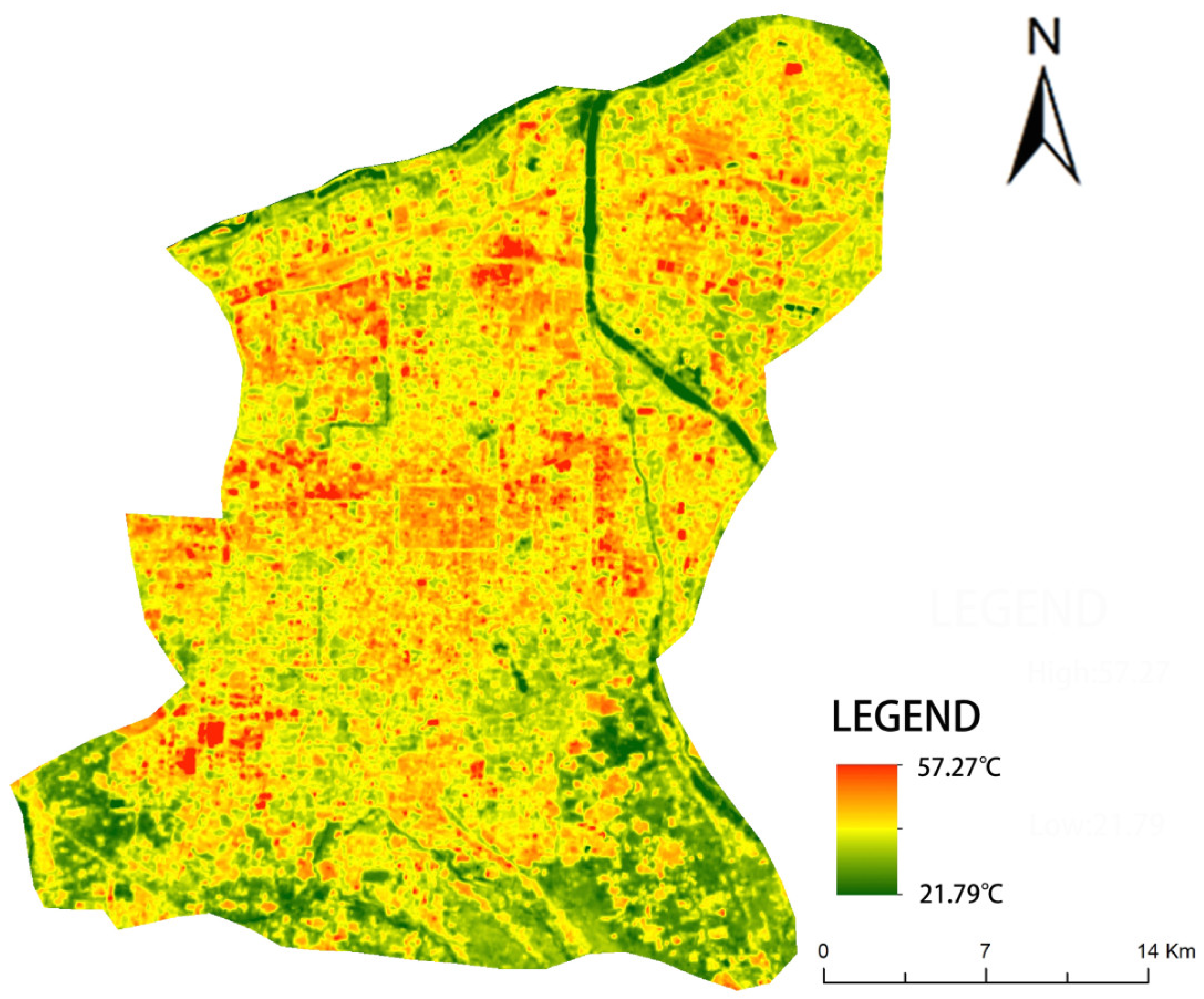
2.2. Land Surface Temperature (LST) Retrieval

On 11 February 2013, NASA successfully launched the Landsat-8 satellite. The satellite carries a total of two sensors, namely the Operational Land Imager (OLI) and the Thermal Infrared Sensor (TIRS), each with a spatial resolution of 30 m [40,41]. The Landsat-8 satellite data have been widely applied in various fields, including urban planning and land use [42,43,44,45]. In the present study, the Landsat-8 satellite images captured during the summer of 2021 were selected as the input data for land surface temperature retrieval. The selected image data correspond to 15 August 2021, a day characterized by stable weather conditions. There were low wind speeds and no precipitation the day before, with minimal impact on the overall thermal environment, and the image showed a cloud cover of less than 0.03%. Various features were clearly distinguished.

Previous studies have indicated that human thermal comfort is directly influenced by both the LST and the atmospheric temperature [46]. However, due to the areal extent of the study area, it is difficult to obtain the necessary atmospheric temperature data from weather station records or field observations. Consequently, the present study used the LST as a representative measure of the urban thermal environment.

Previous research has also shown that the land surface temperature can be calculated by using the radiation transfer equation [47,48]. This approach involves estimating the atmospheric impact on the surface thermal radiation and subtracting this value from the total thermal radiation observed by satellite sensors to derive the surface thermal radiation intensity. This intensity is then converted into the corresponding land surface temperature by using the formula given here as Equation (1):

$$B(T_S)=\lfloor L_{\lambda }-L_{\mathrm{atm},\mathrm{i}}\uparrow -\tau (1-\epsilon )L_{\mathrm{atm},\mathrm{i}}\downarrow \rfloor /\tau \epsilon$$

(1)

where B(T_s) is the black-body radiation corresponding to the specific LST (T_s), L_λ is the thermal infrared radiation brightness value received by the satellite sensor, ε is the land surface emissivity, and τ is the atmospheric transmittance in the thermal infrared band. For the present study, the ε value was calculated by using the Band Math tool in the ENVI 5.3 software. The specific calculation formula is given as follows Equation (2), where Pv represents the Vegetation Coverage, which is calculated using Equation (3). In Equation (3), NDVI stands for normalized difference vegetation index, which is calculated using the NDVI calculation tool in the Toolbox. NDVIS represents the NDVI value in areas with completely bare soil or no vegetation coverage, while NDVIV represents the NDVI values of pixels that are completely covered by vegetation, i.e., the NDVI values of pure vegetation pixels. Using the empirical values of NDVIV = 0.70 and NDVIS = 0.05, if the NDVI of a pixel is greater than 0.70, the value of Pv is set to 1, and if the NDVI is less than 0.05, the value of Pv is set to 0.

$$\epsilon =0.004P\mathrm{v}+0.986$$

(2)

$$P\mathrm{v}=\left[\right(\mathrm{NDVI}-\mathrm{NDVIS})/(\mathrm{NDVIV}-\mathrm{NDVIS}\left)\right]$$

(3)

The τ and atmospheric downward radiation (L_atm,i ↓) and upward radiation (L_atm,i ↑) were estimated using the AtmCorr website “http://atmcorr.gsfc.nasa.gov/ (accessed on 20 May 2022)”. After the B(T_s) value had been obtained, the specific LST was calculated by using Equation (4):

$$T_S=K_2/\ln \left(K_1/B(T_S)+1)\right)$$

(4)

In the Landsat-8 image, K₁ = 774.89 W/(m² μm sr) and K₂ = 1321.08 K. The results of the LST retrieval process are shown in Figure 2.

2.3. Sample Green Space Selection

The present study excluded several specific types of green spaces based on the following considerations. According to China’s relevant regulation, the Standard for Planning of Urban Green Space (GB/T 51346–2019) [49], urban green space is categorized into the following four types: (i) public parks, (ii) green buffers, (iii) square spaces, and (iv) attached green spaces. Among these, the green buffers were excluded from the present study due to the stringent requirements for their locations, layouts, and shapes, along with the challenges involved in formulating detailed quantitative indicators. Additionally, attached green spaces were excluded because they are typically planned and designed in the detailed construction planning stage and do not participate in the balance of urban construction land. Meanwhile, due to their low green space ratios, square spaces cannot provide the same cooling effect as other green spaces (and even bare spaces with no vegetation can have the opposite effect) [50,51], making them irrelevant to the core aim of the present study.

The category of the public park is further subdivided into comprehensive parks, specific parks, community parks, and street gardens. According to the relevant regulations, a single comprehensive park is planned to have an area greater than 10 hectares, while the unique contents or forms of specific parks make it difficult to discuss their optimal size solely from an ecological perspective. Consequently, these two categories are omitted from the present study. Thus, within the public park category, the focus of the present study is narrowed down to community parks and street gardens as the primary research subjects, with the goal of determining their optimal sizes.

Based on high-resolution Google Earth images, the present study used manual vectorization within the ArcGIS 10.3 software to delineate the boundary vectors of the selected sample green spaces. The principles guiding the selection of the sample green spaces included (i) accounting for differences in size between various green spaces; (ii) ensuring a certain distance between each selected sample green space to prevent mutual interference; (iii) avoiding large areas of water within 50 m of each selected green space to ensure data accuracy; and (iv) considering the presence or absence of water bodies within each community park, along with the cooling effect of any water body present. Based on these principles, 20 community parks with water bodies, 20 community parks without water bodies, and 30 street gardens were selected as the research samples. The specific locations of the selected green space samples are shown in Figure 3.

2.4. Analysis of the Cooling Effects of Urban Green Spaces

The present study used the concept of the urban cold island, which is the difference in LST between a patch of green space and its surrounding urban areas [52]. To assess the cooling effects of each patch of green space, the following three indicators were employed: (i) the cooling intensity, (ii) the cooling range, and (iii) the cooling outcome. The cooling intensity represents the difference in LST between the green patch and the turning point of the first drop in LST outside the patch. The cooling range is defined as the distance from the edge of the green patch to the first turning point of cooling. The cooling outcome combines the cooling intensity and cooling range, thereby serving as a comprehensive index for evaluating the cooling effect of the green space. It treats each individual green space as a point, and treats the cooling effect of each individual green space as the volume of a cylinder with a radius equal to its cooling range and a height equal to its cooling intensity. The calculation formula is given here as Equation (5):

$$E=\pi \ast f{(x)}^2\ast T$$

(5)

where E is the cooling outcome of the selected green space, T is the cooling intensity of the green space, and f(x) is the regression function of the cooling intensity and cooling range for the selected sample green space based on its type of green space. To enhance the accuracy of the study, the regression equation with the highest correlation was selected after multiple regressions.

To calculate the cooling outcome of each patch of green space, the study initially computed the average LST within each selected green patch. Subsequently, various buffer zones were established with a radius of 30 m for each type of green space patch in order to quantify the cooling effect of each patch. Finally, the cooling intensity and cooling range were calculated for each patch of green space in order to determine the cooling outcome of each green space.

2.5. Selection of Landscape Indicators

Previous studies have indicated that the cooling effect of a green space is influenced by various factors, with the most significant being the background temperature, size, and shape complexity of the green space [53,54,55,56]. In the present study, a linear regression analysis was used to investigate the relationship between the following selection of landscape indicators and the cooling effect of each green space on both the patch and landscape sizes: (i) the background temperature (i.e., the average LST within each green space patch), (ii) the patch area (i.e., the area of each patch of green space), and (iii) the landscape shape index (LSI), which describes the shape complexity of the green space These indicators were selected because they are the primary factors influencing the cooling effect of each green space, they can effectively capture the spatial characteristics of each patch of green space, they hold significance in both theoretical and practical aspects, and they are easily obtainable and calculable. In particular, the landscape shape index is calculated by using Equation (6):

$$LSI=\frac{0.25E}{\sqrt{A}}$$

(6)

where E is the perimeter of the patch (m) and A is the area of the patch (m²). The LSI of a circular patch is equal to 1, and the LSI of a square patch is equal to 1.13. The larger the LSI value, the more complex the shape of the patch.

2.6. Calculation of the Optimal Size of the Green Space

The present study introduces the concept of the cooling outcome, as defined in Section 2.4, to calculate the optimal size of the green space more comprehensively by considering both the cooling intensity and the cooling range.

First, the ArcGIS 10.3 software was used to compute the cooling intensity and cooling range for each sample green space from the LST data. Then, based on the classification of each green space, the SPSS 21 software was used to conduct a regression analysis on the cooling intensity and cooling range data for each type of green space. After that, the regression model with the highest correlation was selected from the analysis results and incorporated into Equation (5) for calculation, thereby determining the cooling outcome for each type of green space. Finally, the area of each type of green space and its corresponding cooling outcome were subjected to regression analysis in the SPSS software, and the regression model with the highest correlation was selected in order to calculate the optimal size for each type of green space.

3. Results

3.1. Basic Information about Green Spaces in the Study Area

The basic information about the overall green space in the study area is given in

Table 1. Basic information about the overall green space in Xi’an between 2009 and 2019.

Land Type	Green Space Coverage (%)	Ave. Background Temperature (°C)	Ave. Cooling Intensity (°C)	Ave. Cooling Range (m)	Ave. LSI a	Ave. NDVI b
Construction		39.34	–	–	–	–
Urban green space (total)	25.46	37.76	1.53	196.5	1.12	–
Selected community parks with water	–	37.27	2.44	240	1.11	0.43
Selected community parks without water	–	37.69	1.29	184.5	1.13	0.53
Street gardens	–	38.31	0.86	165	1.13	0.43

^a Landscape shape index; ^b normalized difference vegetation index.

below.

As indicated in Table 1, the average background temperature of urban construction land in the study area during the summer of 2021 was 39.34 °C. Following the recommendations of the ISO-7243 standard [57], which assumes individuals are dressed in summer clothing (0.5 clo), the safe wet bulb globe temperature (WBGT) limit for human leisure conditions is 32 to 33 °C. Prolonged exposure to environmental WBGT values beyond this range necessitates safety measures to prevent thermal harm to individuals. Therefore, it is imperative for Xi’an to implement heat prevention measures in order to safeguard the health and safety of residents during the summer.

Compared to urban construction land, the average background temperature of community park land is significantly lower, while the average background temperature of street garden land is only slightly lower. Table 1 also demonstrates the robust cooling effect of urban green space, with an average cooling intensity of 1.53 °C and an average cooling range of 196.5 m. Moreover, the cooling effect of each type of urban green space is seen to decrease in the following order: community parks with water > community parks without water > street gardens. In detail, community parks without water have the highest average normalized vegetation index (NDVI) of 0.53, while both community parks with water and street gardens have average NDVI values of about 0.43, thereby indicating average vegetation growth within these green spaces. Generally speaking, an effective heat prevention measure during urban planning would be to increase the construction of urban green spaces. These green spaces reduce the temperature of the surrounding environment and provide people with a cool place to relax.

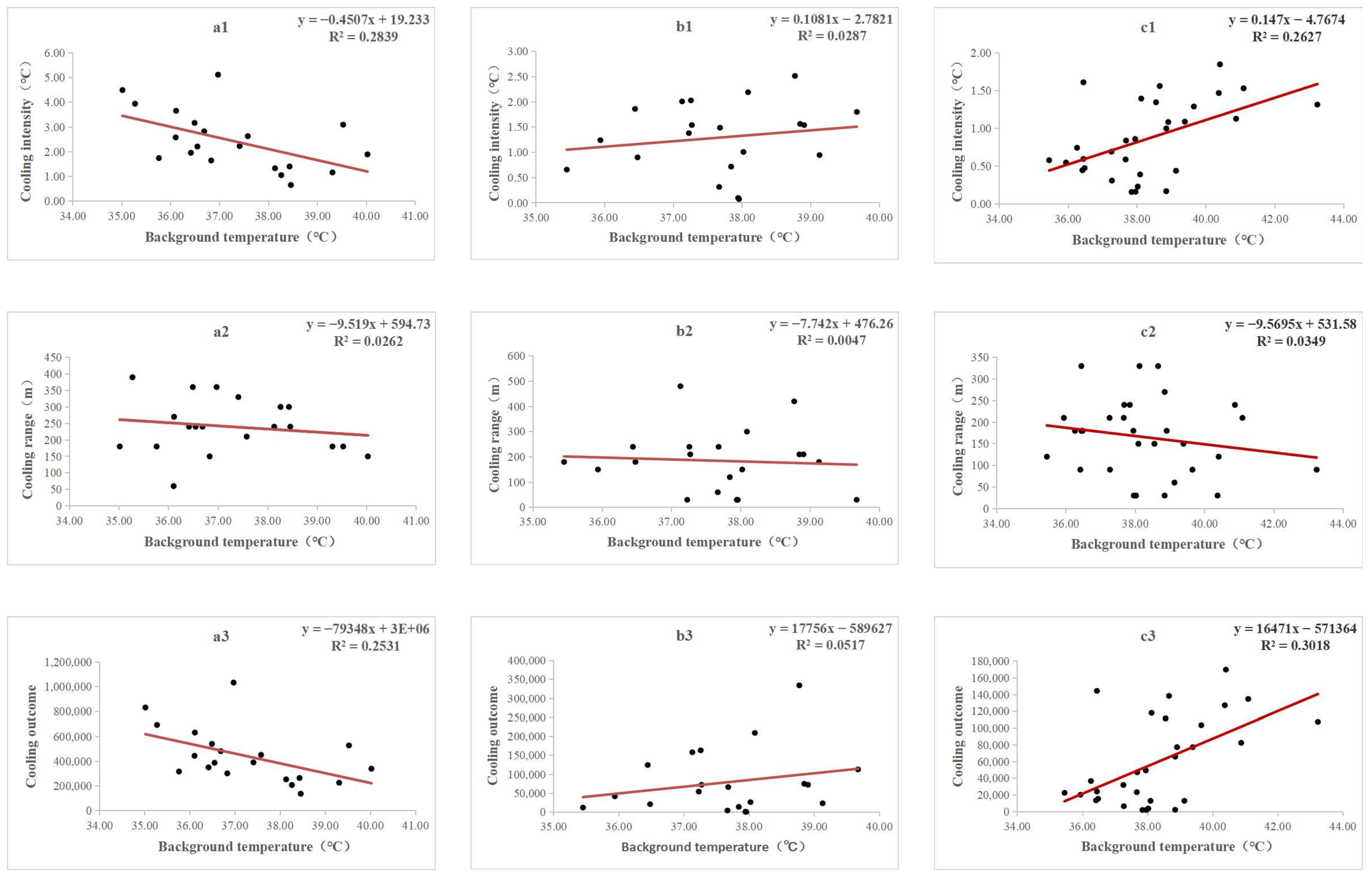
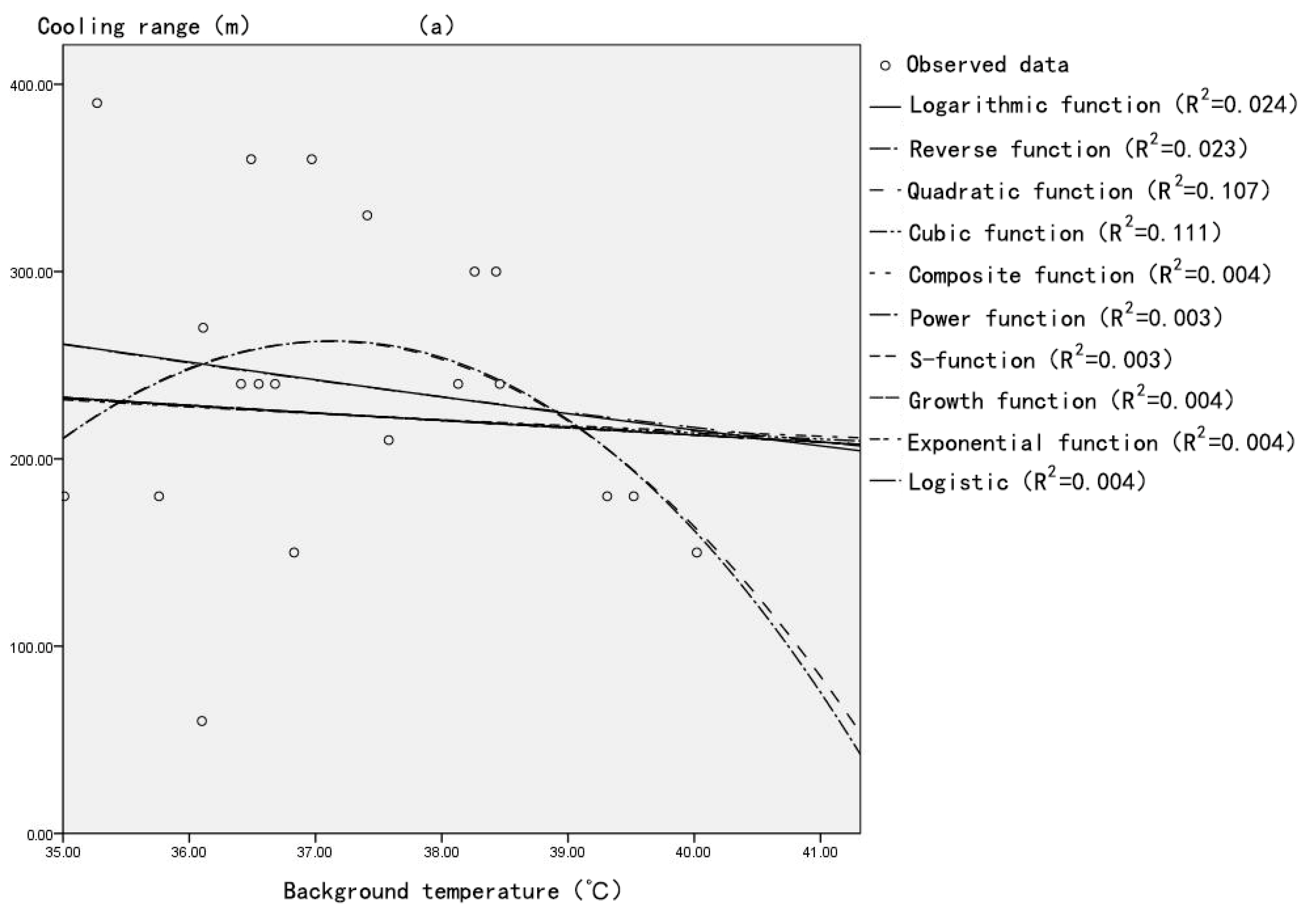
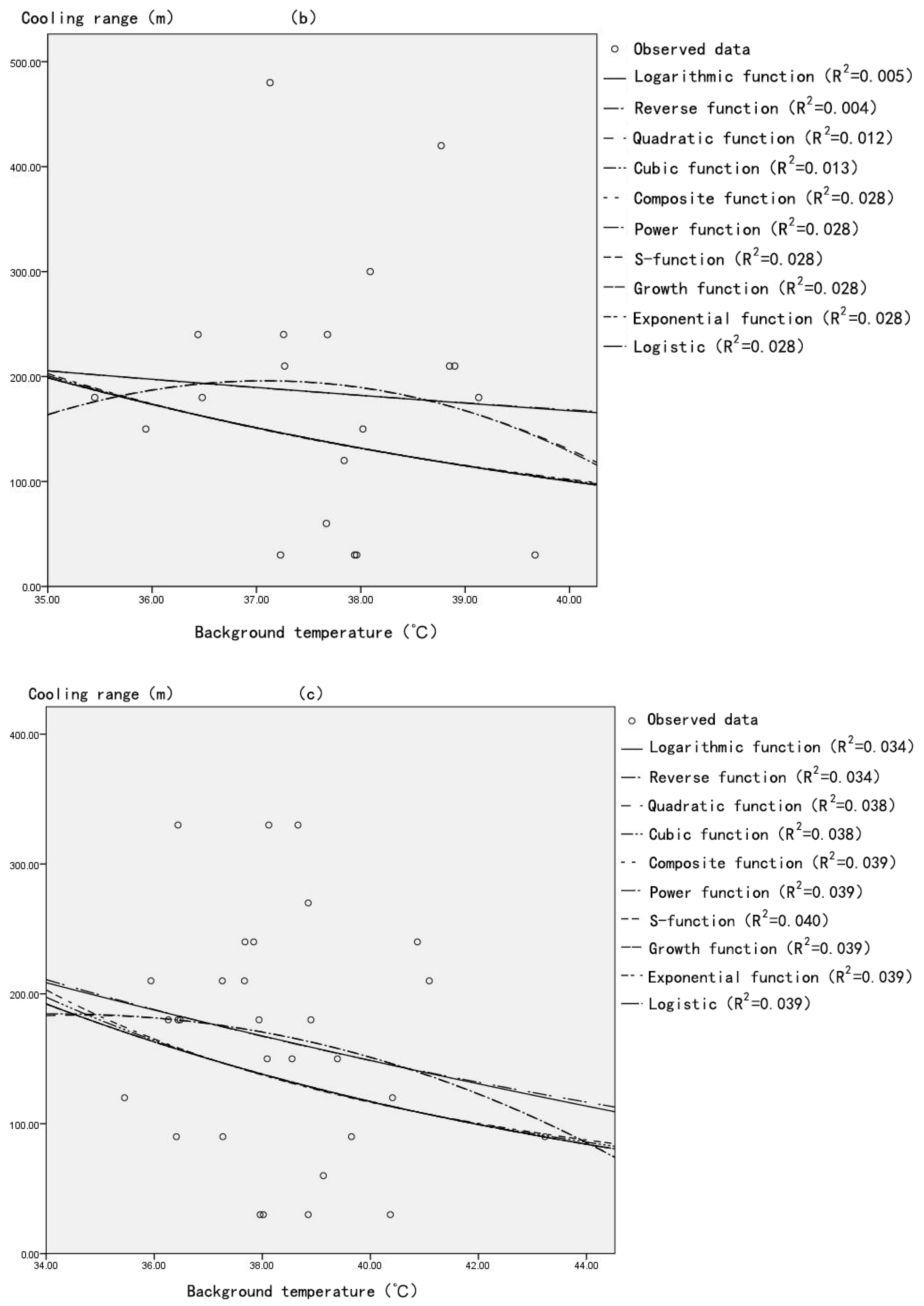
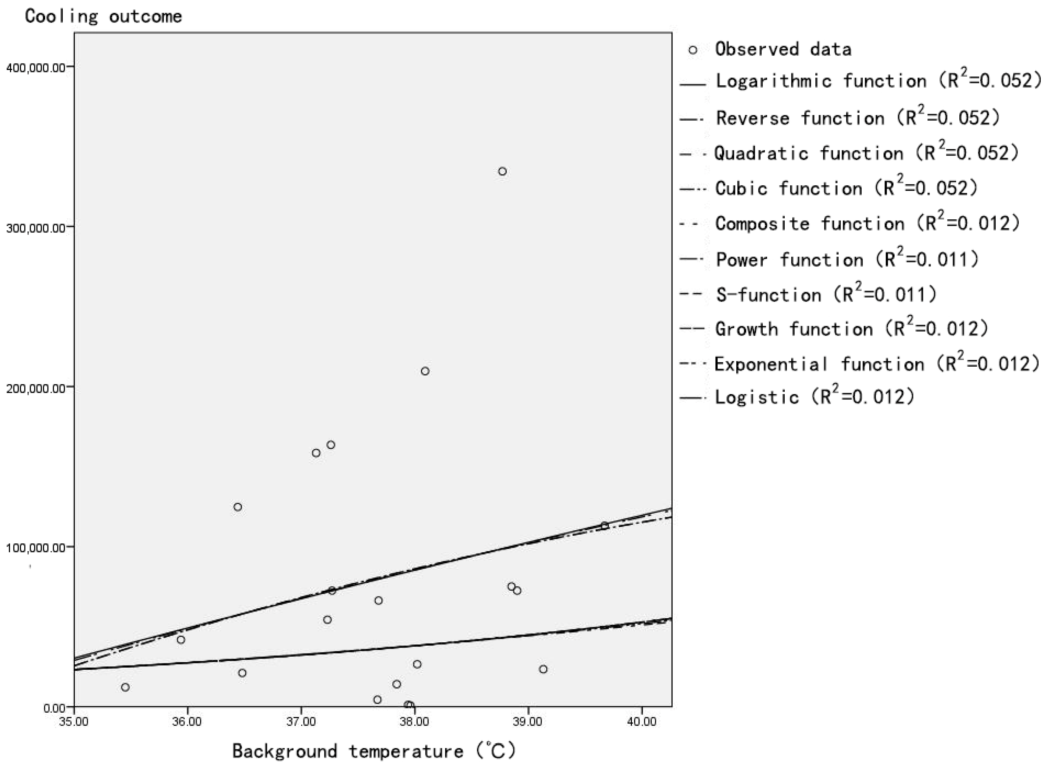
3.2. The Impact of Background Temperature of Green Space on Its Cooling Intensity, Cooling Range, and Cooling Outcome

The results of the regression analysis performed for the cooling intensity and cooling range of three different types of urban green spaces are presented in Figure 4 below. Here, the highest correlation between cooling intensity and cooling range for all three types of urban green space is observed when a quadratic regression function is used. The corresponding R² values for community parks with water, community parks without water, and street gardens are 0.244, 0.592, and 0.269, respectively, and all of the p values are less than or equal to 0.05. The specific functions for community parks with water, community park without water, and street gardens are given as Equations (7)–(9), respectively:

$$Y=12.90{\mathrm{X}}^2-51.98\mathrm{X}+272.52$$

(7)

$$Y=16.23{\mathrm{X}}^2+103.40\mathrm{X}+37.51$$

(8)

$$Y=-100.56{\mathrm{X}}^2+255.21\mathrm{X}+43.68$$

(9)

These expressions were then substituted into Equation (5) in order to determine the cooling outcome of each individual green space.

The results of a linear regression analysis between the background temperature and the cooling intensities, cooling ranges, and cooling outcomes of each type of urban green space in the study area are presented in Figure 5. Here, a distinct relationship between the background temperature and the cooling intensity is observed for each type of green space. Thus a negative linear correlation between background temperature and cooling intensity is shown for community parks with water (Figure 5(a1); R² = 0.28, p ≤ 0.05), whereas a positive linear correlation between background temperature and cooling intensity is displayed for street gardens (Figure 5(c1); R² = 0.26, p ≤ 0.05). Meanwhile, no linear correlation exists between the background temperature of community parks without water and their cooling intensity (Figure 5(b1)). Meanwhile, there is no evident linear correlation between the background temperature and cooling range for either the community parks with water (Figure 5(a2); R² = 0.0003), community parks without water (Figure 5(b2); R² = 0.005), or street gardens (Figure 5(c2); R² = 0.03). Further, in the case of background temperature versus cooling outcome, the community parks with water exhibit a negative linear correlation (Figure 5(a3); R² = 0.25, p ≤ 0.05), while street gardens exhibit a positive linear correlation (Figure 5(c3); R² = 0.30, p ≤ 0.05), and community parks without water exhibit no linear correlation (Figure 5(b3)).

In the case of community parks without water, the results of a non-linear regression analysis between the background temperature and cooling intensity are presented in Figure 6. Here, as with the linear regression analysis (Figure 5(b1)), the non-linear analysis reveals no clear correlation between the background temperature and cooling intensity of the community park without water. Taken together, these results suggest that the background temperature of a community park without water is independent of its cooling intensity.

Further, the results of non-linear regression analyses between the background temperatures and cooling ranges of all three types of green spaces are presented in Figure 7. Here, it can be seen that no non-linear correlation exists between the background temperature and cooling range of any of the selected types of green spaces. Taken together with the results in Figure 5(a3)–(c3), this suggests that the background temperature of a green space does not directly influence its cooling range.

Furthermore, the results of a non-linear regression analysis between background temperature and cooling outcome for the community parks without water are presented in Figure 8. Taking the results in Figure 5(b3) and Figure 8 together, it can be inferred that the background temperature of a community park without water is not correlated with its cooling outcome.

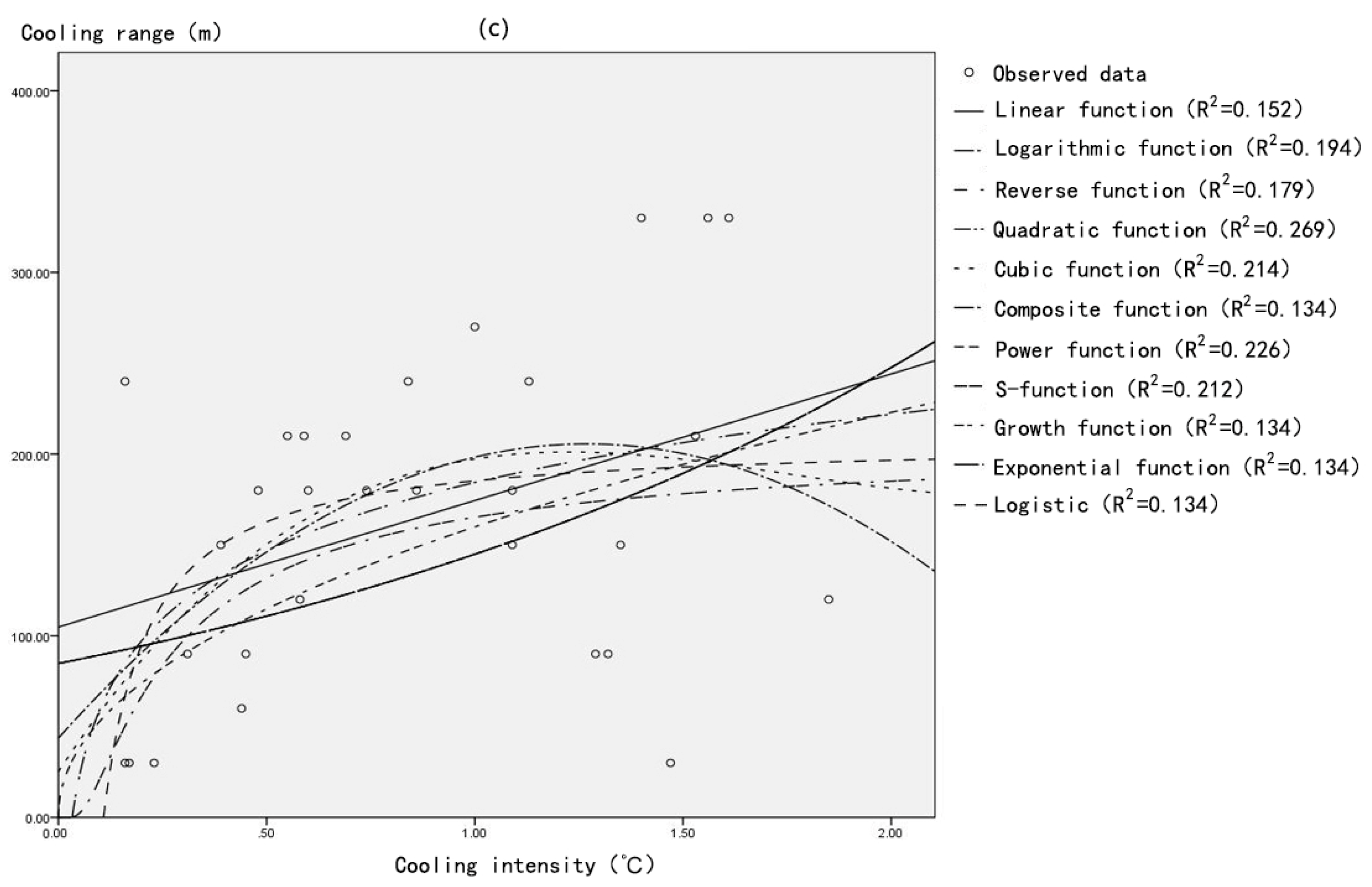
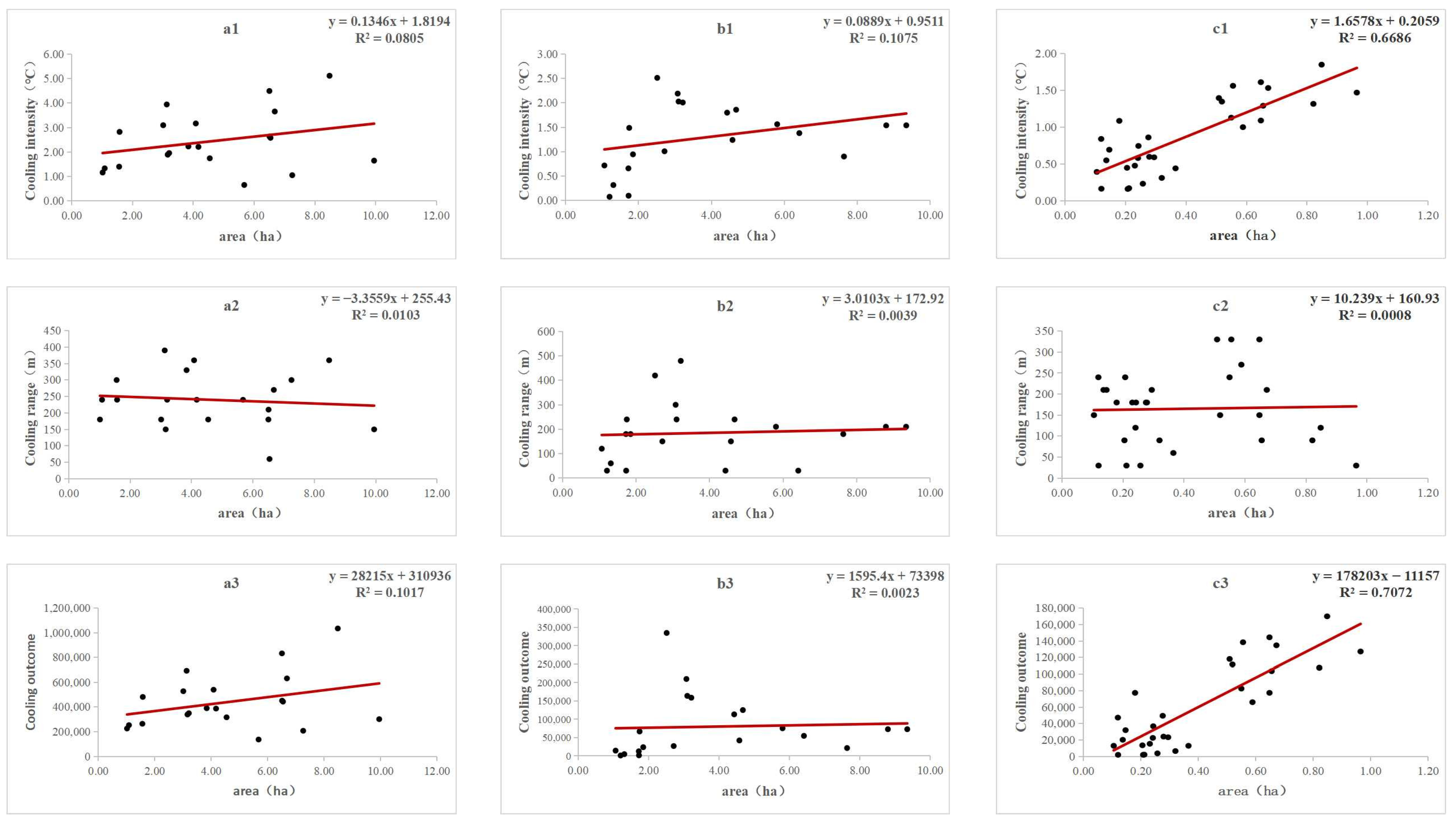
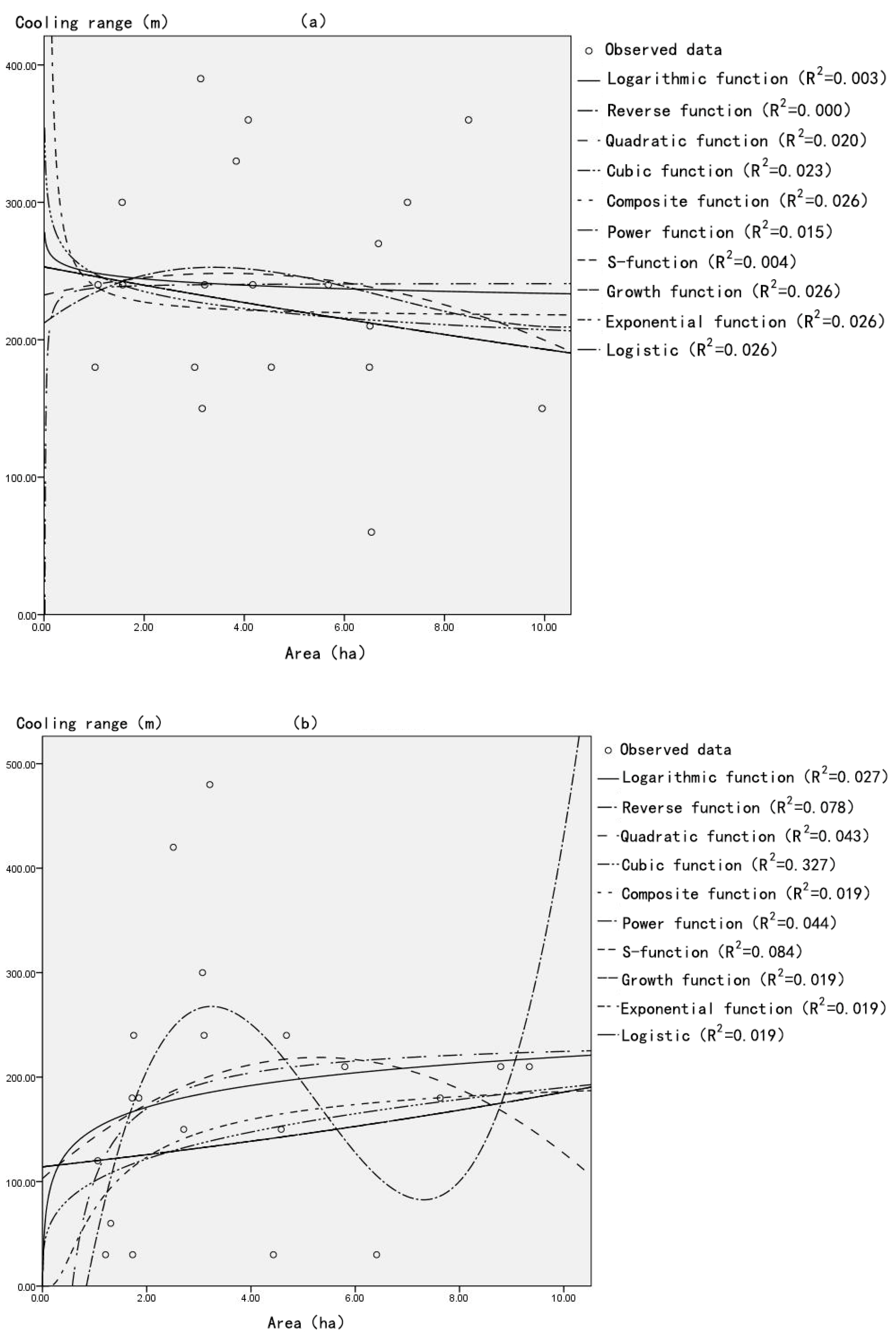
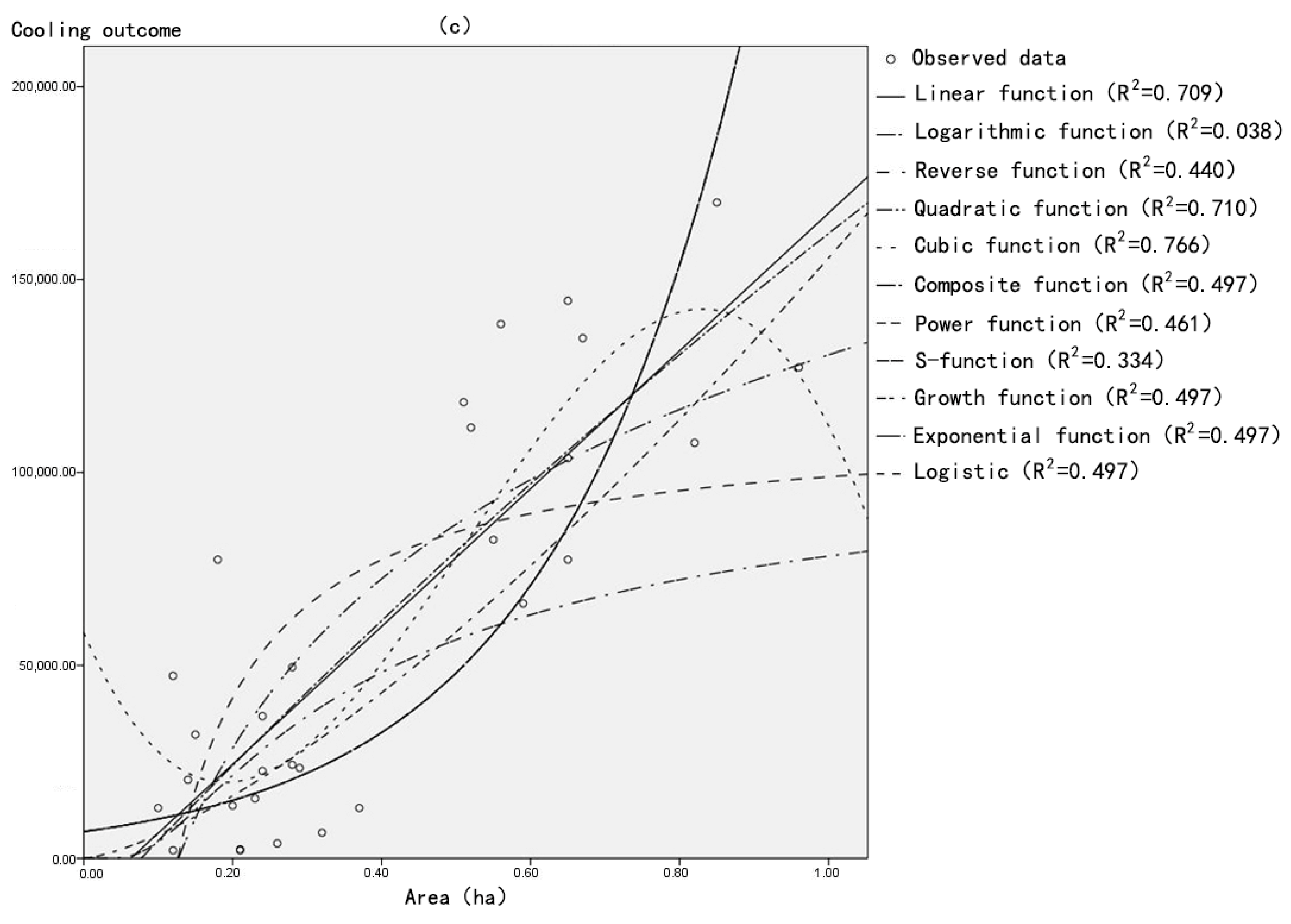
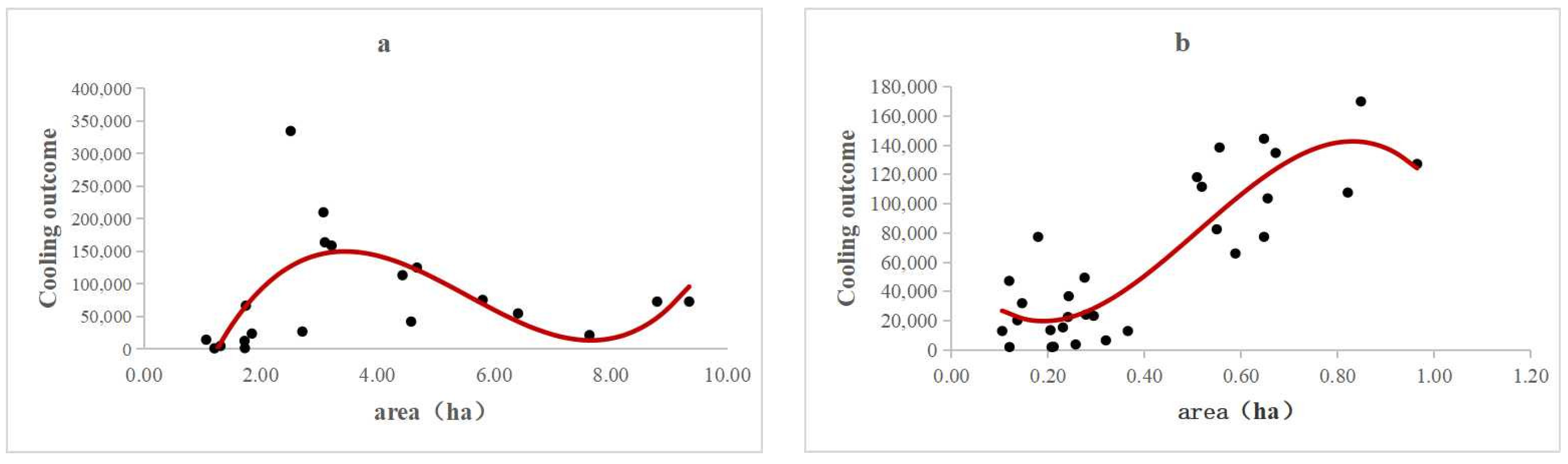
3.3. The Impact of Green Space Area on Its Cooling Intensity, Cooling Range, and Cooling Outcome

The results of linear regression analyses between the area of each type of urban green space and its corresponding cooling intensity, cooling range, and cooling outcome are presented in Figure 9. Here, no linear correlation is observed between the cooling intensity and the areas of community parks with water (Figure 9(a1); R² = 0.1) or without water (Figure 9(b1); R² = 0.11). However, there is a significant positive linear correlation between the area of street gardens and their cooling intensity (Figure 9(c1); R² = 0.67, p ≤ 0.05). In other words, for smaller urban green spaces, a larger area corresponds to a higher cooling intensity. Meanwhile, no linear correlations are observed between the cooling range and area of community parks with water (Figure 9(a2); R² = 0.01), community parks without water (Figure 9(b2); R² = 0.0039), or street gardens (Figure 9(c2); R² = 0.0008). In addition, there are no linear correlations between the cooling effects and areas of the community parks with water (Figure 9(a3); R² = 0.1) or without water (Figure 9(b3); R² = 0.0023). However, there is a significantly positive linear correlation between the area of the street garden and its cooling outcome (Figure 9(c3); R² = 0.71, p ≤ 0.05).

The non-linear regression analyses of the relationships between the cooling intensities and areas of community parks with or without water are shown in Figure 10. Here, there is no non-linear correlation between the area of the community park with water and its cooling intensity (Figure 10a), which may be due to the cooling effects of the water bodies within such green spaces. In the case of community parks without water, however, a non-linear correlation between area and cooling intensity is observed (Figure 10b), with the regression curve exhibiting a cubic function (R² = 0.611, p ≤ 0.05). This result reveals that the cooling intensity of the community park without water initially increases, then decreases, and then increases again as the area of this type of green space increases.

Furthermore, the non-linear regression analyses for the relationship between the area of each type of green space and its corresponding cooling range are presented in Figure 11. Here, it is evident that there is no non-linear correlation between the area and cooling range of community parks with water (Figure 11a), thereby indicating that the area of community park with water is not related to its cooling range. By contrast, there is a non-linear correlation between the area and cooling range of both the community park without water (Figure 11b) and the street garden (Figure 11c), with both regression curves exhibiting the highest correlations for cubic functions (R² = 0.327 and 0.261, respectively; p ≤ 0.05). In detail, the cooling range of the community park without water initially increases, then decreases, and subsequently increases again as the area of the green space increases. Conversely, the cooling range of the street garden initially decreases, then increases, and subsequently decreases again as the area increases. For more detailed insights, a further non-linear regression analysis is provided in Section 3.5.

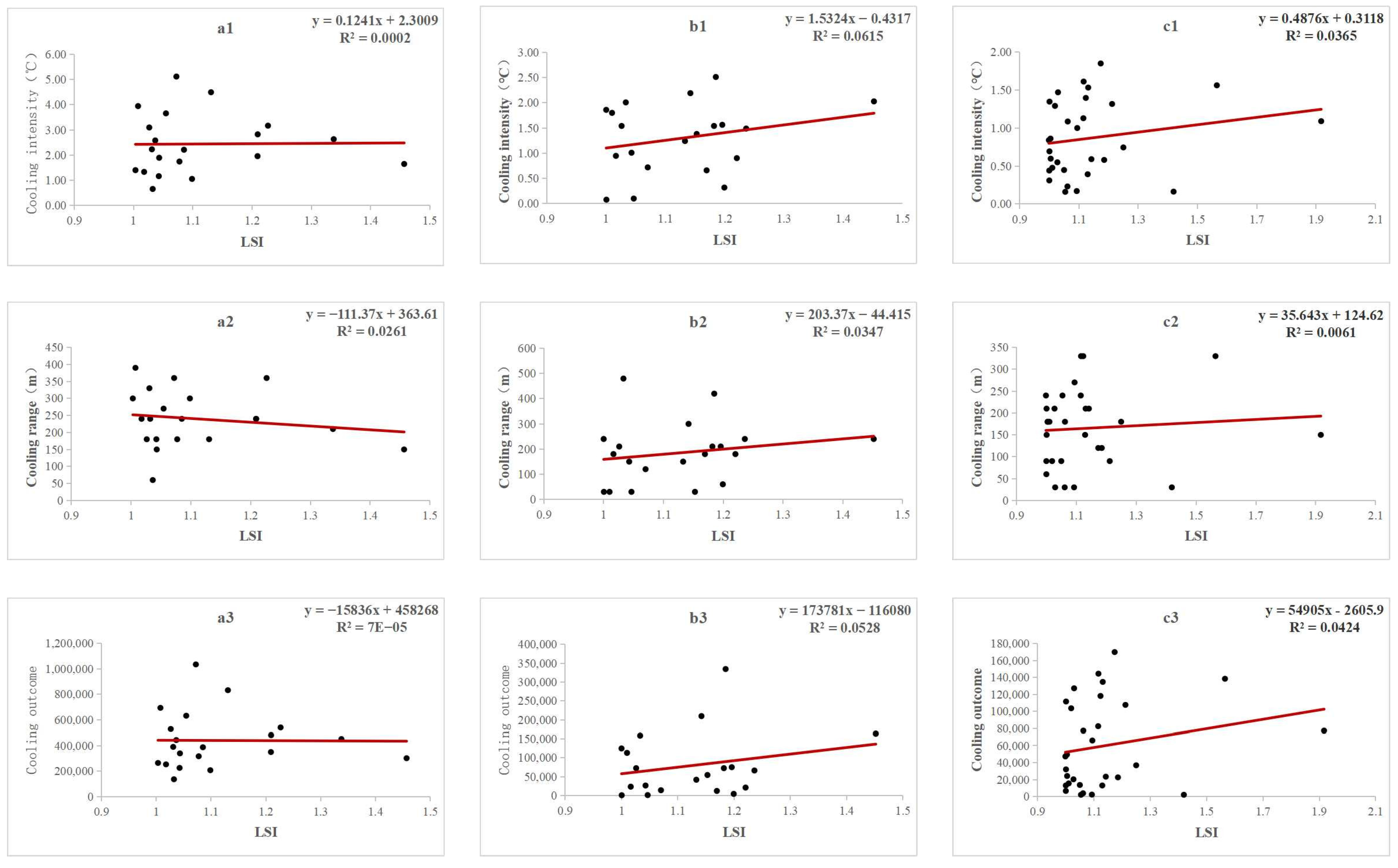
3.4. The Impact of Green Space Landscape Shape Index (LSI) on Its Cooling Intensity, Cooling Range, and Cooling Outcome

The linear regression analyses of the relationships between the LSI of each urban green space type and its corresponding cooling intensity, cooling range, and cooling outcome are shown in Figure 12, and the corresponding non-linear regression analyses are presented in Figure 13. An examination of the trends in these figures clearly reveals that the shape of each type of urban green space has no direct impact on its cooling effect.

3.5. Calculation of the Optimal Size of Green Spaces

Based on the above comprehensive assessment of the cooling effects of various green spaces, the present study has identified the cooling outcome as the key indicator reflecting the cooling impact of urban green spaces. The results in Figure 9 clearly illustrate that not all types of urban green spaces exhibit highly linear relationships between their areas and cooling outcomes. Consequently, this section presents the results of further non-linear regression analyses on the relationship between the area of each type of green space and its cooling outcome. The model with the highest correlation based on the regression results is then selected in order to calculate the optimal area of each type of green space.

The results of the non-linear regression analyses for the relationship between the areas and cooling outcomes of the three distinct types of urban green spaces are presented in Figure 14. Here, an exceedingly weak correlation is observed between the area and cooling outcome for community parks with water (Figure 14a), thereby suggesting the absence of an optimal size. Meanwhile, the function with the highest correlation between the area and cooling effect of the community park without water is a cubic function, as expressed by Equation (10):

Y = 3634.14X³ − 60510.73X² + 287365.45X − 270979.71

(10)

with an R² value of 0.419 (p ≤ 0.05). The corresponding function is plotted in Figure 15a.

In the case of the street garden, the function with the highest correlation between area and cooling effect is also a cubic function, and is represented by Equation (11):

Y = −933778.94X³ + 1429595.13X² − 442282.15X + 58506.35

(11)

with an R² value of 0.766 (p ≤ 0.05). The corresponding function is plotted in Figure 15b.

An examination of Figure 15a in conjunction with Equation (10) reveals that the coefficient of the cubic term in Equation (11) is greater than 0, the coefficient of the quadratic term is less than 0, and the equation satisfies the condition of γ < β²/3α, where α, β, and γ are the three roots of the equation in order of numerical size. Therefore, when the equation is plotted, a positive N-shaped curve is obtained. Our calculations reveal the one real root of this function to be 1.24, and the derivative function of Equation (10) provides the solutions 3.44 and 7.66, with Δ > 0, where Δ is the discriminant of root. This result indicates that the model has three monotonic intervals. Consequently, when the area of a community park without water is less than 3.44 hectares, its cooling outcome increases with the increase in green space area; when the area is in the range of 3.44–7.66 hectares, the cooling outcome decreases as the green space area increases, and when the green space area exceeds 7.66 hectares, the cooling outcome resumes its initial increase with the increase in green space area.

Meanwhile, an examination of Figure 15b in conjunction with Equation (11) indicates that the coefficient of the cubic term Equation (11) is less than 0, the coefficient of the quadratic term is greater than 0, and the equation satisfies the condition γ > β²/3α. Therefore, the plotted curve takes the form of an inverted N. Our calculations reveal the one real root of this function to be 1.17, and its derivative function has the solutions 0.19 and 0.83, with Δ > 0, thereby indicating that the model has three monotonic intervals. Therefore, when the area of a street garden is below 0.19 hectares, the cooling outcome decreases as the area of green space increases. When the area of a street garden is in the range of 0.19 to 0.83 hectares, however, the cooling outcome increases with the increase in green space area. Finally, when the green space area exceeds 0.83 hectares, the cooling outcome of the street garden decreases as the green space area is increased.

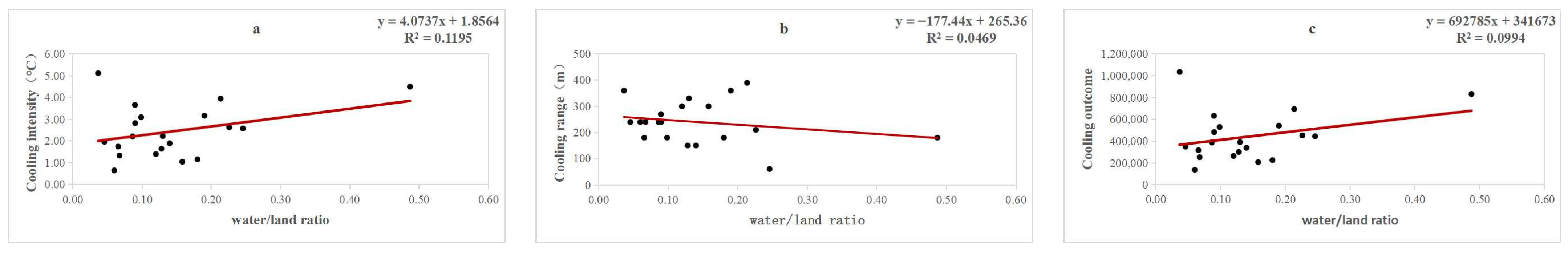
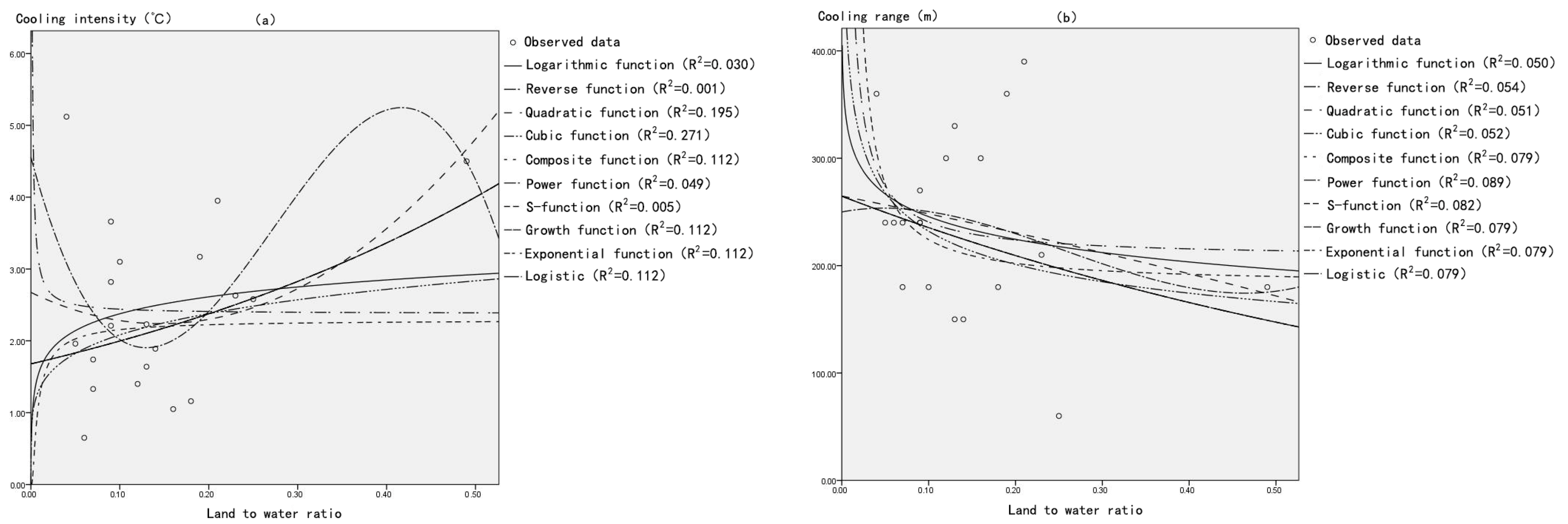
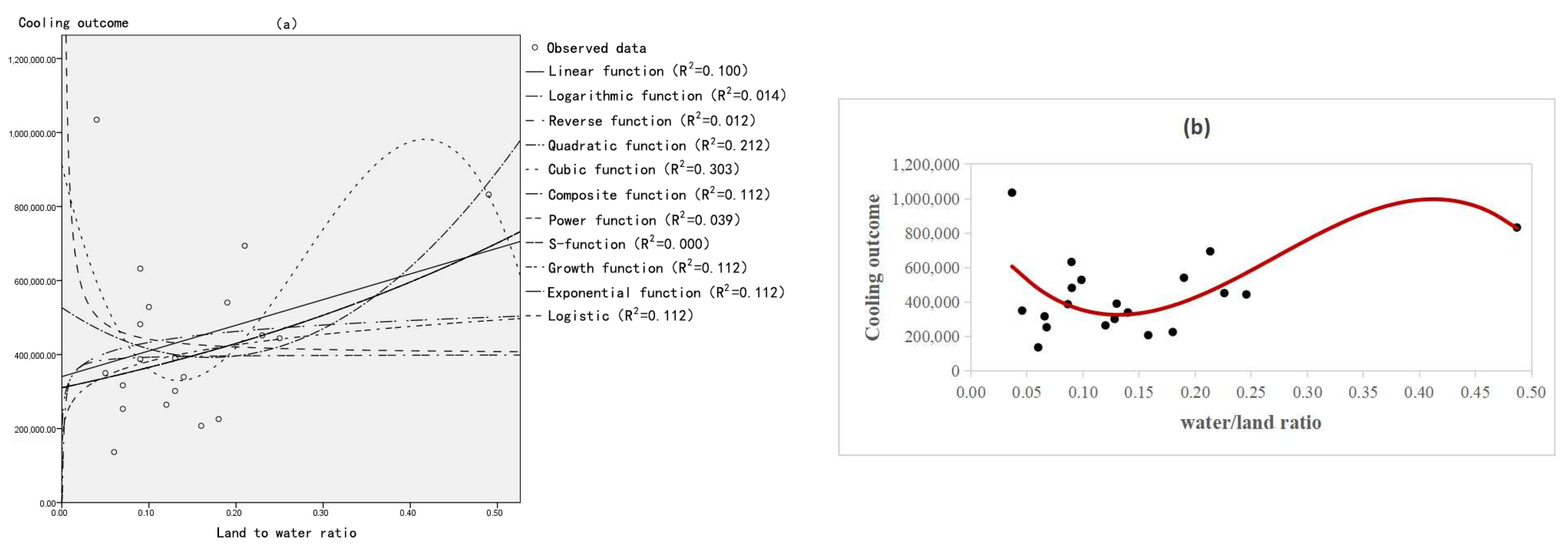
3.6. The Effects of Water/Land Ratio on the Cooling Intensity, Cooling Range, and Cooling Outcome of the Community Park with Water; Calculation of the Optimal Water/Land Ratio

Water possesses a high specific heat capacity along with a low thermal conductivity, thus making evaporation the primary cooling mechanism for a water body [58]. These characteristics lead to a significant reduction in the sensible heat transfer capacity of water, thereby altering the heat transfer pattern and giving rise to the phenomenon known as the constant temperature effect. This effect contributes to a more stable climate, including a lower maximum temperature and a higher minimum temperature [26]. Therefore, the presence of internal water bodies in a community park may result in the absence of an optimal green space area. However, a new quantitative indicator, namely, the water/land ratio, can be used to further explore the relationships between the area of water within the green space and its background temperature, cooling intensity, cooling range, and cooling outcome. The water/land ratio refers to the ratio of water area to the total area of green space (including green area and a small portion of building and road paving area) within a patch of urban green space.

The effects of the water/land ratio on the cooling intensity, cooling range, and cooling outcome of the community park with water are revealed by the linear regression analysis in Figure 16. Here, no linear correlation is observed between the water/land ratio of the community park with water and either its cooling intensity (Figure 16a; R² = 0.12), cooling range (Figure 16b; R² = 0.05), or cooling outcome (Figure 16c; R² = 0.10).

By contrast, the results in Figure 17a reveal a non-linear correlation between the water/land ratio of the community park with water and its cooling intensity. Here, the regression curve with the highest correlation is a cubic function (R² = 0.271, p ≤ 0.05). Thus, as the area of water in the community park continues to increase, the cooling intensity first decreases, then increases, and then decreases again. Meanwhile, the water/land ratio of a community park with water is unrelated to its cooling range (Figure 17b).

Based on the above findings, a non-linear regression analysis was performed on the relationship between the water/land ratio and cooling outcome of the community park with water, and the function with the highest correlation was selected as the model function in order to determine the optimum water/land ratio. The results in Figure 18a reveal a non-linear relationship between the water/land ratio and the cooling outcome, with the highest correlation being observed for the cubic function given in Equation (12):

Y = −57811930.41X³ + 47814517.11X² − 9720282.74X + 912738.81

(12)

with an R² value of 0.316 (p ≤ 0.05). This function graph is plotted in Figure 18b.

Thus, an examination of Equation (12) and Figure 18b indicates that the coefficient of the cubic term in Equation (12) is less than 0, the coefficient of the quadratic term is greater than 0, and the equation satisfies the condition γ > β²/3α. Consequently, the plotted curve takes the form of an inverted N. Our calculation shows that the one real root of this function is 0.58, and the solutions of the corresponding derivative function are 0.134 and 0.417, with Δ > 0, thereby indicating that the model has three monotonic intervals. Thus, when the water/land ratio of the community park is below 0.134, the cooling outcome decreases as the proportion of water within the green space increases. When the ratio is in the range of 0.134 to 0.417, however, the cooling outcome increases as the proportion of water within the green space increases. Finally, when the water/land ratio exceeds 0.417, the cooling outcome decreases as the green space to water/land ratio increases.

4. Discussion

4.1. The Relationship between Landscape Indicators and the Cooling Intensities, Cooling Ranges, and Cooling Outcomes of Green Spaces

Based on the above results, the relationships between the various landscape indicators and the cooling intensities, cooling ranges, and cooling outcomes of the three types of urban green spaces in the study area are summarized in

Table 2. The relationship between various landscape indicators and the cooling intensities, cooling ranges, and cooling outcomes of the three types of urban green spaces in the study area.

Type of Green Space	Background Temperature versus Cooling Intensity	Background Temperature versus Cooling Range	Background Temperature versus Cooling Outcome	Area versus Cooling Intensity	Area versus Cooling Range	Area versus Cooling Outcome	LSI versus Cooling Intensity	LSI versus Cooling Range	LSI versus Cooling Outcome
Community parks with water	Negative linear correlation	No correlation	Negative linear correlation	No correlation	No correlation	No correlation	No correlation	No correlation	No correlation
Community parks without water	No correlation	No correlation	No correlation	Non-linear correlation	Non-linear correlation	Non-linear correlation	No correlation	No correlation	No correlation
Street gardens	Positive linear correlation	No correlation	Positive linear correlation	Positive linear correlation	Non-linear correlation	Non-linear correlation	No correlation	No correlation	No correlation

.

As noted in Table 1 (Section 3.1), the average background temperature of urban green spaces in the study area is 37.76 °C, which represents a 1.58 °C reduction compared to the average background temperature of urban construction land. Specifically, the average background temperatures of community parks with and without water are, respectively, 2.07 and 1.65 °C lower than the average background temperature of urban construction land. Additionally, the average background temperature of street gardens is 1.03 °C lower than that of urban construction land. These data confirm the substantial cooling impacts of the various green spaces. It is important to highlight that the internal configuration and structure of each green space plays a pivotal role in its cooling capability. In particular, larger green spaces typically feature more abundant greenery and water bodies, along with three-dimensional structures and planar features. Consequently, the cooling effects (columns 2, 3, and 4 of Table 2) of these green spaces are inversely proportional to the average background temperature of each green space type. As a result, community parks larger than 1 hectare exhibit lower background temperatures and are cooler than smaller street gardens with areas of less than 1 hectare. Furthermore, as street gardens are often smaller and more open, with lower amounts of internal green coverage, direct exposure to sunlight is more likely, thus leading to higher surface temperatures. Moreover, research has shown that the cooling effect of a water body is typically more pronounced when the surrounding temperature is elevated [59]. Consequently, the higher the background temperature within a community park with water, the greater the cooling impact of the water body. This leads to a negative correlation between the background temperature of a community park with water and its cooling intensity and cooling outcome (row 2 of Table 2). Meanwhile, there is no clear correlation between the background temperature of the community park without water and its cooling intensity and cooling outcome (row 3 of Table 2). Similarly, there is no evident correlation between the background temperatures of all three green spaces and their cooling ranges (column 3 of Table 2). This lack of correlation may be due to the intricate internal conditions of the green spaces, including the spatial layout along with the presence of water bodies and hard paving within the green space [60]. Additionally, the complex urban construction environment outside the green space, along with the construction conditions, could contribute to this phenomenon [61,62].

In terms of area, only the street garden exhibits a positive linear correlation with its cooling intensity and cooling outcome (columns 5 and 7, Table 2). A larger area implies that the street garden has more green space coverage, a higher vegetation density, and more effective shading. Consequently, the cooling intensity and cooling outcome of this type of green space are gradually increased as the area increases. In the case of the community parks with water, no correlation between the area and the cooling intensity and cooling outcome of the green space is evident. Furthermore, based on Figure 17 and Figure 18, it is apparent that the proportional area of internal water in this type of green space exerts a more substantial influence on its cooling outcome. Meanwhile, for community parks without water, the results in Figure 9, Figure 10, Figure 11 and Figure 14 indicate that there is no linear correlation between the green space area and its cooling intensity, cooling range and cooling outcome. Notably, the cubic function model, as the non-linear regression model with the highest correlation, best captures the relationship between green area and its cooling effect. This observation aligns well with the research undertaken by Peng et al. and Cheng et al. [35,63]. Specifically, the cooling effect of this type of green space does not consistently increase or decrease with its area; rather, there is a trend of an initial increase, followed by decrease, and a subsequently renewed increase in the cooling effect. The physical interpretation of this result may be closely related to the reasons discussed below. In smaller green spaces, the shading effects and evapotranspiration of trees and other vegetation can significantly reduce the surface temperature within and around the green space [64]. As the area of green space increases, the overall evapotranspiration of the green space also increases, and a higher vegetation coverage means that a wider area can benefit from this cooling effect [65,66]. Since the green space is relatively small, the cool air generated can easily cover the interior of the green areas and diffuse from the interior to the peripheral areas with air movements. Therefore, when the green space area is small, its cooling effect gradually increases as the area increases. However, studies have shown that a marginal diminishing effect exists in the cooling effect of green spaces [21]. As the area of green space further increases, the contribution of newly added vegetation to the overall cooling effect gradually decreases. Specifically, when the green space reaches a certain size, a relatively uniform temperature zone may form inside [25]. At this point, heat is redistributed inside the green space through convection and conduction, and the already cooled interior areas transfer some cool air to the hotter edge areas [67]. However, due to the large area of the green space, its cooling effect can only cover the interior areas, making it more difficult for the cool air to diffuse to the peripheral areas, resulting in a relatively weakened cooling effect on the surrounding areas. When the area of green space continues to expand and reaches a larger scale, its internal ecological elements become more diverse, and the distribution of vegetation becomes more uniform. Research has shown that compared to smaller green spaces, larger green spaces had a more significant effect on regulating the surrounding microclimate [68]. This is mainly because larger green spaces have more complex landscape types and a more uniform distribution of vegetation. Existing research has confirmed that these characteristics endow green spaces with stronger cooling effects [69,70]. These strong cooling effects create a more stable microclimate environment, ultimately forming a persistent and stable cold air layer [25]. This cold air layer can fully achieve cooling within the green space and can expand to surrounding areas through effective air flow guidance, thus improving the overall cooling effect of the green space [56].

Moreover, the research findings suggest that there is no correlation between the areas of community parks with water and their cooling ranges, while the areas of street gardens exhibits a weak non-linear correlation with their cooling range (column 6, Table 2). In addition to the effects of water bodies within green spaces, this result may be related to the built environment surrounding the green space. The cooling range is not solely impacted by temperature regulation within the green space itself, but is closely tied to the surrounding environment, including thermal radiation from nearby buildings, heat absorption from adjacent roads, building density, building height, floor area ratio, etc. [61,62]. These factors may not be directly related to the area of the green space, but they all play a role in affecting its cooling range. Finally, the vegetation coverage and quality within the green space can also influence its cooling range [59]. Given that the average NDVI values of the selected green spaces are not high, simply increasing the green space area without improving the quality of vegetation therein may not lead to a linear increase in the cooling effect; in fact, it may have a negative impact.

The results in columns 8–10 of Table 2 indicate that there are no correlations between the LSI values of the three different types of urban green spaces and their cooling intensities and cooling ranges. Previous research on the effects of the shapes of green spaces on their cooling effects has been contentious, with some scholars arguing that the cooling effect of a green space is positively related to the complexity of its shape [21], and others holding the opposite view [71]. In the present study, a thorough examination of the shape complexity of the selected green spaces revealed that the average LSI of each green space was low, at only 1.12. This is attributed to the predominant division of green space in the study area based on the urban square road network. Most of the green space patches exhibit regular square shapes, possess distinct artificial features, lack natural forms, and exhibit a low complexity. Consequently, the present study found no correlation between the LSI of green space and its cooling effect.

4.2. The Optimal Size and Water/Land Ratio

The results in Figure 14 (Section 3.4) indicate that both the community parks without water and the street gardens have optimal sizes, while the community parks with water do not. According to Equation (10) and Figure 15a, when the area of a community park without water is less than 3.44 hectares, the cooling outcome increases as the green space area increases. When the green space area is between 3.44 and 7.66 hectares, however, the cooling outcome starts to decrease with the increase in the green space area. Finally, once the green space area exceeds 7.66 hectares, the cooling outcome begins to increase with the further increase in the green space area. Therefore, the optimal size for a community park without water is found to be 3.44 hectares.

Conversely, in the case of the street garden, Equation (11) and Figure 15b indicate that the cooling outcome decreases with an increase in green space area when this is less than 0.19 hectares. Then, when the green space area is between 0.19 and 0.83 hectares, the cooling outcome begins to increase with the green space area. Finally, when the green space area exceeds 0.83 hectares, the cooling outcome resumes its initial decrease with the increase in the green space area. Therefore, the optimal size for the street garden is 0.83 hectares.

For a community park with water, a determination of the optimal size is challenging due to the influence of the internal water bodies. However, further examination revealed that this type of green space exhibits an optimal water/land ratio of 0.417 (Equation (12), Figure 18b). In practical terms, when the water body within a community park with water constitutes approximately 29.43% of the total park area, the park can achieve its highest cooling efficiency. This finding aligns with the conclusion drawn by Feng et al., who suggested that a green space attains a better cooling effect when the proportion of internal water is around 30% [72].

4.3. Guidance on Urban Green Space System Planning in Xi’an

The present study approach provides useful methods and strategies to assist urban planners in determining the necessary amount of green space in order to achieve widespread cooling in an urban area. This is crucial for ensuring the efficient cooling effects of green spaces. The results offer valuable guidance for urban planners, thereby enabling them to make well-informed decisions, especially in situations where land resources are limited. The specific guiding principles are as follows:

(1) To attain the most effective cooling impact and ensure widespread and sustained cooling in Xi’an, it is recommended that the area of water in the community parks with water should ideally account for 29.41% of the total area. For the community parks without water, efforts should be made to maintain an area of approximately 3.44 hectares. Similarly, recreational gardens should aim for an area of around 0.83 hectares in order to optimize their cooling efficiency.

(2) The cooling effects of water bodies should be fully utilized, as these are widely acknowledged to be crucial ecological components of urban areas due to their substantial capacity to mitigate the surface UHI [73]. Indeed, the present study’s findings affirm that green spaces with water bodies have more robust cooling effects than those without. However, owing to the constrained water resources in Xi’an, the prevalence of green spaces with water bodies is relatively limited. Therefore, priority should be accorded to incorporating strategically planned water bodies during future green space planning and redevelopment initiatives, in order to maximize the cooling potential of those green spaces. However, it is crucial to recognize that, while enhancing the cooling intensity, an indiscriminate increase in the area of water bodies within the green spaces may diminish the overall cooling efficiency [74]. Therefore, based on the outcomes of the present study, the optimal cooling effects of green spaces can be achieved by ensuring that the water body within the green space constitutes 11.82–29.43% of the total area, and by striving to approach the upper limit for maximal effectiveness.

It should be noted that the cooling efficacy of water bodies is also intricately linked to the conditions of the surrounding greenery [75]. Hence, the optimal use of greenery can synergistically enhance the cooling impact of the water bodies, thereby augmenting the overall cooling effects of the urban green spaces. Conversely, in instances where there is insufficient greenery surrounding the water body, and the prevalence of buildings is high, such that the water body is completely enveloped by buildings to create a basin-like landscape, the heat exchange capacity between the water body and the surrounding environment will be limited. This scenario can compromise the cooling effectiveness of the urban green spaces with water [76]. Therefore, in addition to adhering to a clearly defined water/land ratio, green space planners should also prioritize the suitable configuration of the landscape around the water body. This involves ensuring that the water body is surrounded by ample green space, and avoiding any excessive intrusion by tall buildings. Lastly, the type of greenery around water bodies is also crucial. Studies indicate that trees, due to their strong shading capability, provide more significant cooling effects compared to grasslands and shrubs [77,78]. Moreover, small-leaved plants exhibit better cooling performance compared to large-leaved ones [79]. These are all factors that planners need to consider.

5. Conclusions

With a focus on mitigating the surface urban heat island (UHI) effect, the present study used Xi’an as a case study to investigate the optimal sizes of various types of green spaces in order to maximize their cooling effects in urban areas. Firstly, the study confirmed that urban green spaces exhibit a notable cooling effect, and revealed the relationship between three landscape indicators, namely background temperature, patch area, and landscape shape index, and the cooling intensity, cooling range, and cooling outcome of three types of green spaces. Furthermore, through calculations, the study determined the optimal sizes of three different types of green spaces, with the optimal size of a community park without water being found to be 3.44 hectares and that of a street garden being 0.83 hectares. In addition, while no optimal size exists for the community park with water, this type of green space exhibits an optimal water/land ratio of 0.417. Finally, the study proposed guidance for the planning of the green space system in Xi’an.

However, due to constraints such as limited research time, challenges in data acquisition, and constraints on manpower and material resources, the study has some limitations and requires further refinement. Specifically, numerous factors influence the cooling effects of urban green spaces. In addition to water bodies, scholars have identified that human-made indicators such as building height, building density, and street direction impact the cooling effect and optimal size of the green space [80]. Therefore, in future research, a comprehensive consideration and in-depth analysis and discussion of the additional factors that influence the cooling effects of urban green spaces should be conducted. Furthermore, for green spaces with water, factors such as the location and shape of the internal water body can also influence the cooling effect of the entire green space. Therefore, future research should focus on exploring and accurately quantifying the cooling effects of internal water bodies within green spaces, and on proposing methods and suggestions to guide the future planning and design of urban green spaces.

In conclusion, the present study has introduced a novel approach for determining the optimal sizes of various types of urban green spaces, particularly in the context of the prevalent UHI effect and limited land availability in the city. These findings are expected to provide valuable insights for planners and administrators not only in Xi’an, but also in other cities. The intention is to provide scientific guidance for urban climate adaptability planning and urban green space system planning. By doing so, this study contributes to the alleviation of the UHI effect and facilitates the rational allocation of urban land resources.

References

1. Antrop, M. Landscape change and the urbanization process in Europe. Landsc. Urban Plan. 2004, 67, 9–26. [Google Scholar] [CrossRef]
2. Pang, B.; Zhao, J.; Zhang, J.; Yang, L. Calculating optimal scale of urban green space in Xi’an, China. Ecol. Indic. 2023, 147, 110003. [Google Scholar] [CrossRef]
3. Huang, H.; Deng, X.; Yang, H.; Li, S.; Li, M. Spatial evolution of the effects of urban heat island on residents’ health. Teh. Vjesn. 2020, 27, 1427–1435. [Google Scholar]
4. Jiang, L.; O’Neill, B.C. Global urbanization projections for the Shared Socioeconomic Pathways. Glob. Environ. Chang. 2017, 42, 193–199. [Google Scholar] [CrossRef]
5. Kong, F.; Yin, H.; Wang, C.; James, P. A satellite image-based analysis of factors contributing to the green-space cool island intensity on a city scale. Urban For. Urban Green. 2014, 13, 846–853. [Google Scholar] [CrossRef]
6. Fan, C.; Myint, S.W.; Zheng, B. Measuring the spatial arrangement of urban vegetation and its impacts on seasonal surface temperatures. Prog. Phys. Geogr. 2015, 39, 199–219. [Google Scholar] [CrossRef]
7. Aram, F.; García, E.H.; Solgi, E.; Mansournia, S. Urban green space cooling effect in cities. Heliyon 2019, 5. [Google Scholar] [CrossRef] [PubMed]
8. Takano, T.; Nakamura, K.; Watanabe, M. Urban residential environments and senior citizens’ longevity in megacity areas: The importance of walkable green spaces. J. Epidemiol. Community Health 2002, 56, 913–918. [Google Scholar] [CrossRef] [PubMed]
9. Xiao, X.D.; Dong, L.; Yan, H.; Yang, N.; Xiong, Y. The influence of the spatial characteristics of urban green space on the urban heat island effect in Suzhou Industrial Park. Sustain. Cities Soc. 2018, 40, 428–439. [Google Scholar] [CrossRef]
10. Chung, C.K.L.; Zhang, F.; Wu, F. Negotiating green space with landed interests: The urban political ecology of greenway in the Pearl River Delta, China. Antipode 2018, 50, 891–909. [Google Scholar] [CrossRef]
11. Jiao, H.; Li, C.; Yu, Y.; Peng, Z. Urban public green space equity against the context of high-speed urbanization in Wuhan, central China. Sustainability 2020, 12, 9394. [Google Scholar] [CrossRef]
12. Peng, W.; Wang, R.; Duan, J.; Gao, W.; Fan, Z. Surface and canopy urban heat islands: Does urban morphology result in the spatiotemporal differences? Urban Clim. 2022, 42, 101136. [Google Scholar] [CrossRef]
13. Ali, J.M.; Marsh, S.H.; Smith, M.J. Modelling the spatiotemporal change of canopy urban heat islands. Build. Environ. 2016, 107, 64–78. [Google Scholar] [CrossRef]
14. Hu, Y.; Hou, M.; Jia, G.; Zhao, C.; Zhen, X.; Xu, Y. Comparison of surface and canopy urban heat islands within megacities of eastern China. ISPRS J. Photogramm. Remote Sens. 2019, 156, 160–168. [Google Scholar] [CrossRef]
15. Deilami, K.; Kamruzzaman, M.; Liu, Y. Urban heat island effect: A systematic review of spatio-temporal factors, data, methods, and mitigation measures. Int. J. Appl. Earth Obs. Geoinf. 2018, 67, 30–42. [Google Scholar] [CrossRef]
16. Zhou, D.; Xiao, J.; Bonafoni, S.; Berger, C.; Deilami, K.; Zhou, Y.; Frolking, S.; Yao, R.; Qiao, Z.; Sobrino, J.A. Satellite remote sensing of surface urban heat islands: Progress, challenges, and perspectives. Remote Sens. 2018, 11, 48. [Google Scholar] [CrossRef]
17. Yang, J.; Gong, P.; Zhou, J.X.; Huang, H.B.; Wang, L. Detection of the urban heat island in Beijing using HJ-1B satellite imagery. Sci. China Earth Sci. 2010, 53, 67–73. [Google Scholar] [CrossRef]
18. Gao, Y.; Chang, M.; Zhao, J. Research on temporal and spatial variation of heat island effect in Xi’an, China. Appl. Ecol. Environ. Res. 2019, 17, 231–244. [Google Scholar] [CrossRef]
19. Tsou, J.; Zhuang, J.; Li, Y.; Zhang, Y. Urban heat island assessment using the Landsat 8 data: A case study in Shenzhen and Hong Kong. Urban Sci. 2017, 1, 10. [Google Scholar] [CrossRef]
20. Liu, S.; Zang, Z.; Wang, W.; Wu, Y. Spatial-temporal evolution of urban heat Island in Xi’an from 2006 to 2016. Phys. Chem. Earth Parts A/B/C 2019, 110, 185–194. [Google Scholar] [CrossRef]
21. Yu, Z.; Guo, X.; Jørgensen, G.; Vejre, H. How can urban green spaces be planned for climate adaptation in subtropical cities? Ecol. Indic. 2017, 82, 152–162. [Google Scholar] [CrossRef]
22. Yu, Z.; Xu, S.; Zhang, Y.; Jørgensen, G.; Vejre, H. Strong contributions of local background climate to the cooling effect of urban green vegetation. Sci. Rep. 2018, 8, 6798. [Google Scholar] [CrossRef] [PubMed]
23. Le, M.T.; Cao, T.A.T.; Tran, N.A.Q. The role of green space in the urbanization of Hanoi city. In E3S Web of Conferences; EDP Sciences: Les Ulis, France, 2019; Volume 97, p. 01013. [Google Scholar]
24. Yang, G.; Yu, Z.; Jørgensen, G.; Vejre, H. How can urban blue-green space be planned for climate adaption in high-latitude cities? A seasonal perspective. Sustain. Cities Soc. 2020, 53, 101932. [Google Scholar] [CrossRef]
25. Yu, Z.; Yang, G.; Zuo, S.; Jørgensen, G.; Koga, M.; Vejre, H. Critical review on the cooling effect of urban blue-green space: A threshold-size perspective. Urban For. Urban Green. 2020, 49, 126630. [Google Scholar] [CrossRef]
26. Pang, B.; Zhao, J.; Zhang, J.; Yang, L. How to plan urban green space in cold regions of China to achieve the best cooling efficiency. Urban Ecosyst. 2022, 25, 1181–1198. [Google Scholar] [CrossRef]
27. Masoudi, M.; Tan, P.Y.; Liew, S.C. Multi-city comparison of the relationships between spatial pattern and cooling effect of urban green spaces in four major Asian cities. Ecol. Indic. 2019, 98, 200–213. [Google Scholar] [CrossRef]
28. Wang, C.; Ren, Z.; Dong, Y.; Zhang, P.; Guo, Y.; Wang, W.; Bao, G. Efficient cooling of cities at global scale using urban green space to mitigate urban heat island effects in different climatic regions. Urban For. Urban Green. 2022, 74, 127635. [Google Scholar] [CrossRef]
29. Masoudi, M.; Tan, P.Y.; Fadaei, M. The effects of land use on spatial pattern of urban green spaces and their cooling ability. Urban Clim. 2021, 35, 100743. [Google Scholar] [CrossRef]
30. Kong, F.; Yin, H.; James, P.; Hutyra, L.; He, H.S. Effects of spatial pattern of greenspace on urban cooling in a large metropolitan area of eastern China. Landsc. Urban Plan. 2014, 128, 35–47. [Google Scholar] [CrossRef]
31. Shah, A.; Garg, A.; Mishra, V. Quantifying the local cooling effects of urban green spaces: Evidence from Bengaluru, India. Landsc. Urban Plan. 2021, 209, 104043. [Google Scholar] [CrossRef]
32. Naeem, S.; Cao, C.; Qazi, W.A.; Zamani, M.; Wei, C.; Acharya, B.K.; Rehman, A.U. Studying the association between green space characteristics and land surface temperature for sustainable urban environments: An analysis of Beijing and Islamabad. ISPRS Int. J. Geo-Inf. 2018, 7, 38. [Google Scholar] [CrossRef]
33. Han, D.; Xu, X.; Qiao, Z.; Wang, F.; Cai, H.; An, H.; Jia, K.; Liu, Y.; Sun, Z.; Wang, S.; et al. The roles of surrounding 2D/3D landscapes in park cooling effect: Analysis from extreme hot and normal weather perspectives. Build. Environ. 2023, 231, 110053. [Google Scholar] [CrossRef]
34. Du, C.; Jia, W.; Chen, M.; Yan, L.; Wang, K. How can urban parks be planned to maximize cooling effect in hot extremes? Linking maximum and accumulative perspectives. J. Environ. Manag. 2022, 317, 115346. [Google Scholar] [CrossRef] [PubMed]
35. Peng, J.; Dan, Y.; Qiao, R.; Liu, Y.; Dong, J.; Wu, J. How to quantify the cooling effect of urban parks? Linking maximum and accumulation perspectives. Remote Sens. Environ. 2021, 252, 112135. [Google Scholar] [CrossRef]
36. Ren, W.; Zhao, J.; Ma, X.; Wang, X. Analysis of the spatial differentiation and scale effects of the three-dimensional architectural landscape in Xi’an, China. PLoS ONE 2021, 16, e0261846. [Google Scholar] [CrossRef] [PubMed]
37. Wang, C.; Zhang, H.; Ma, Z.; Yang, H.; Jia, W. Urban Morphology Influencing the Urban Heat Island in the High-Density City of Xi’an Based on the Local Climate Zone. Sustainability 2024, 16, 3946. [Google Scholar] [CrossRef]
38. Ma, Y.; Zhao, M.; Li, J.; Wang, J.; Hu, L. Cooling effect of different land cover types: A case study in Xi’an and Xianyang, China. Sustainability 2021, 13, 1099. [Google Scholar] [CrossRef]
39. Chen, H.; Deng, Q.; Zhou, Z.; Ren, Z.; Shan, X. Influence of land cover change on spatio-temporal distribution of urban heat island—A case in Wuhan main urban area. Sustain. Cities Soc. 2022, 79, 103715. [Google Scholar] [CrossRef]
40. Roy, D.P.; Wulder, M.A.; Loveland, T.R.; Woodcock, C.E.; Allen, R.G.; Anderson, M.C.; Helder, D.; Irons, J.R.; Johnson, D.M.; Kennedy, R.; et al. Landsat-8: Science and product vision for terrestrial global change research. Remote Sens. Environ. 2014, 145, 154–172. [Google Scholar] [CrossRef]
41. Sekertekin, A.; Abdikan, S.; Marangoz, A.M. The acquisition of impervious surface area from LANDSAT 8 satellite sensor data using urban indices: A comparative analysis. Environ. Monit. Assess. 2018, 190, 1–13. [Google Scholar] [CrossRef] [PubMed]
42. Pervaiz, W.; Uddin, V.; Khan, S.A.; Khan, J.A. Satellite-based land use mapping: Comparative analysis of Landsat-8, Advanced Land Imager, and big data Hyperion imagery. J. Appl. Remote Sens. 2016, 10, 026004. [Google Scholar] [CrossRef]
43. Keeratikasikorn, C.; Bonafoni, S. Urban heat island analysis over the land use zoning plan of Bangkok by means of Landsat 8 imagery. Remote Sens. 2018, 10, 440. [Google Scholar] [CrossRef]
44. Chaves, M.E.D.; Picoli, M.C.A.; Sanches, I.D. Recent applications of Landsat 8/OLI and Sentinel-2/MSI for land use and land cover mapping: A systematic review. Remote Sens. 2020, 12, 3062. [Google Scholar] [CrossRef]
45. Deliry, S.I.; Avdan, Z.Y.; Avdan, U. Extracting urban impervious surfaces from Sentinel-2 and Landsat-8 satellite data for urban planning and environmental management. Environ. Sci. Pollut. Res. 2021, 28, 6572–6586. [Google Scholar] [CrossRef] [PubMed]
46. Li, Z.L.; Tang, B.H.; Wu, H.; Ren, H.; Yan, G.; Wan, Z.; Trigo, I.F.; Sobrino, J.A. Satellite-derived land surface temperature: Current status and perspectives. Remote Sens. Environ. 2013, 131, 14–37. [Google Scholar] [CrossRef]
47. Yu, X.; Guo, X.; Wu, Z. Land surface temperature retrieval from Landsat 8 TIRS—Comparison between radiative transfer equation-based method, split window algorithm and single channel method. Remote Sens. 2014, 6, 9829–9852. [Google Scholar] [CrossRef]
48. Sekertekin, A. Validation of physical radiative transfer equation-based land surface temperature using Landsat 8 satellite imagery and SURFRAD in-situ measurements. J. Atmos. Sol. Terr. Phys. 2019, 196, 105161. [Google Scholar] [CrossRef]
49. The Standard for Planning of Urban Green Space (GB/T 51346—2019); Ministry of Housing and Urban Rural Development of the People’s Republic of China. China Architecture and Building Press: Beijing, China, 2019.
50. Li, H.; Meng, H.; He, R.; Lei, Y.; Guo, Y.; Ernest, A.; Jombach, S.; Tian, G. Analysis of cooling and humidification effects of different coverage types in small green spaces (SGS) in the context of urban homogenization: A case of HAU campus green spaces in summer in Zhengzhou, China. Atmosphere 2020, 11, 862. [Google Scholar] [CrossRef]
51. Li, H.; Wang, G.; Tian, G.; Jombach, S. Mapping and analyzing the park cooling effect on urban heat island in an expanding city: A case study in Zhengzhou city, China. Land 2020, 9, 57. [Google Scholar] [CrossRef]
52. Półrolniczak, M.; Kolendowicz, L.; Majkowska, A.; Czernecki, B. The influence of atmospheric circulation on the intensity of urban heat island and urban cold island in Poznań, Poland. Theor. Appl. Climatol. 2017, 127, 611–625. [Google Scholar] [CrossRef]
53. Santamouris, M. Cooling the cities—A review of reflective and green roof mitigation technologies to fight heat island and improve comfort in urban environments. Sol. Energy 2014, 103, 682–703. [Google Scholar] [CrossRef]
54. Kuang, W.; Liu, Y.; Dou, Y.; Chi, W.; Chen, G.; Gao, C.; Yang, T.; Liu, J.; Zhang, R. What are hot and what are not in an urban landscape: Quantifying and explaining the land surface temperature pattern in Beijing, China. Landsc. Ecol. 2015, 30, 357–373. [Google Scholar] [CrossRef]
55. Estoque, R.C.; Murayama, Y.; Myint, S.W. Effects of landscape composition and pattern on land surface temperature: An urban heat island study in the megacities of Southeast Asia. Sci. Total Environ. 2017, 577, 349–359. [Google Scholar] [CrossRef] [PubMed]
56. Gunawardena, K.R.; Wells, M.J.; Kershaw, T. Utilising green and bluespace to mitigate urban heat island intensity. Sci. Total Environ. 2017, 584, 1040–1055. [Google Scholar] [CrossRef] [PubMed]
57. ISO 7243:2017; Ergonomics of the Thermal Environment—Assessment of Heat Stress Using the WBGT (Wet Bulb Globe Temperature) Index. ISO: Geneva, Switzerland, 2017.
58. Wu, J.; Li, C.; Zhang, X.; Zhao, Y.; Liang, J.; Wang, Z. Seasonal variations and main influencing factors of the water cooling islands effect in Shenzhen. Ecol. Indic. 2020, 117, 106699. [Google Scholar] [CrossRef]
59. Wang, Y.; Ouyang, W. Investigating the heterogeneity of water cooling effect for cooler cities. Sustain. Cities Soc. 2021, 75, 103281. [Google Scholar] [CrossRef]
60. Zhao, W.; Li, A.; Huang, Q.; Gao, Y.; Li, F.; Zhang, L. An improved method for assessing vegetation cooling service in regulating thermal environment: A case study in Xiamen, China. Ecol. Indic. 2019, 98, 531–542. [Google Scholar] [CrossRef]
61. Hamada, S.; Tanaka, T.; Ohta, T. Impacts of land use and topography on the cooling effect of green areas on surrounding urban areas. Urban For. Urban Green. 2013, 12, 426–434. [Google Scholar] [CrossRef]
62. Zhang, Q.; Zhou, D.; Xu, D.; Rogora, A. Correlation between cooling effect of green space and surrounding urban spatial form: Evidence from 36 urban green spaces. Build. Environ. 2022, 222, 109375. [Google Scholar] [CrossRef]
63. Cheng, X.; Wei, B.; Chen, G.; Li, J.; Song, C. Influence of park size and its surrounding urban landscape patterns on the park cooling effect. J. Urban Plan. Dev. 2015, 141, A4014002. [Google Scholar] [CrossRef]
64. Qiu, G.Y.; Zou, Z.; Li, X.; Li, H.; Guo, Q.; Yan, C.; Tan, S. Experimental studies on the effects of green space and evapotranspiration on urban heat island in a subtropical megacity in China. Habitat Int. 2017, 68, 30–42. [Google Scholar] [CrossRef]
65. Jamei, E.; Rajagopalan, P.; Seyedmahmoudian, M.; Jamei, Y. Review on the impact of urban geometry and pedestrian level greening on outdoor thermal comfort. Renew. Sustain. Energy Rev. 2016, 54, 1002–1017. [Google Scholar] [CrossRef]
66. Lin, W.; Yu, T.; Chang, X.; Wu, W.; Zhang, Y. Calculating cooling extents of green parks using remote sensing: Method and test. Landsc. Urban Plan. 2015, 134, 66–75. [Google Scholar] [CrossRef]
67. Sharma, A.; Conry, P.; Fernando, H.J.S.; Hamlet, A.F.; Hellmann, J.J.; Chen, F. Green and cool roofs to mitigate urban heat island effects in the Chicago metropolitan area: Evaluation with a regional climate model. Environ. Res. Lett. 2016, 11, 064004. [Google Scholar] [CrossRef]
68. Oliveira, S.; Andrade, H.; Vaz, T. The cooling effect of green spaces as a contribution to the mitigation of urban heat: A case study in Lisbon. Build. Environ. 2011, 46, 2186–2194. [Google Scholar] [CrossRef]
69. Zhou, W.; Huang, G.; Cadenasso, M.L. Does spatial configuration matter? Understanding the effects of land cover pattern on land surface temperature in urban landscapes. Landsc. Urban Plan. 2011, 102, 54–63. [Google Scholar] [CrossRef]
70. Rui, L.; Buccolieri, R.; Gao, Z.; Ding, W.; Shen, J. The impact of green space layouts on microclimate and air quality in residential districts of Nanjing, China. Forests 2018, 9, 224. [Google Scholar] [CrossRef]
71. Peng, J.; Xie, P.; Liu, Y.; Ma, J. Urban thermal environment dynamics and associated landscape pattern factors: A case study in the Beijing metropolitan region. Remote Sens. Environ. 2016, 173, 145–155. [Google Scholar] [CrossRef]
72. Feng, X.; Shi, H. Research on the cooling effect of Xi’an parks in summer based on remote sensing. Shengtai Xuebao/Acta Ecol. Sin. 2012, 32, 7355–7363. [Google Scholar]
73. Yao, L.; Sailor, D.J.; Yang, X.; Xu, G.; Zhao, J. Are water bodies effective for urban heat mitigation? Evidence from field studies of urban lakes in two humid subtropical cities. Build. Environ. 2023, 245, 110860. [Google Scholar] [CrossRef]
74. Sun, R.; Chen, L. How can urban water bodies be designed for climate adaptation? Landsc. Urban Plan. 2012, 105, 27–33. [Google Scholar] [CrossRef]
75. Mostofa, T.; Manteghi, G. Influential factors of water body to enhance the urban cooling islands (Ucis): A review. Int. Trans. J. Eng. Manag. Appl. Sci. Technol. 2020, 11, 1–12. [Google Scholar]
76. Perini, K.; Magliocco, A. Effects of vegetation, urban density, building height, and atmospheric conditions on local temperatures and thermal comfort. Urban For. Urban Green. 2014, 13, 495–506. [Google Scholar] [CrossRef]
77. Feyisa, G.L.; Dons, K.; Meilby, H. Efficiency of parks in mitigating urban heat island effect: An example from Addis Ababa. Landsc. Urban Plan. 2014, 123, 87–95. [Google Scholar] [CrossRef]
78. Zölch, T.; Maderspacher, J.; Wamsler, C.; Pauleit, S. Using green infrastructure for urban climate-proofing: An evaluation of heat mitigation measures at the micro-scale. Urban For. Urban Green. 2016, 20, 305–316. [Google Scholar] [CrossRef]
79. Kong, F.; Yan, W.; Zheng, G.; Yin, H.; Cavan, G.; Zhan, W.; Zhang, N.; Cheng, L. Retrieval of three-dimensional tree canopy and shade using terrestrial laser scanning (TLS) data to analyze the cooling effect of vegetation. Agric. For. Meteorol. 2016, 217, 22–34. [Google Scholar] [CrossRef]
80. Akbari, H.; Kolokotsa, D. Three decades of urban heat islands and mitigation technologies research. Energy Build. 2016, 133, 834–842. [Google Scholar] [CrossRef]
Figure 1. The location of the study area.
Land 13 01043 g001
Figure 2. The land surface temperature of the study area in 2021.
Land 13 01043 g002
Figure 3. The distribution of sample green space locations (The numbers are the serial numbers of the sample green spaces).
Land 13 01043 g003
Figure 4. The correlation analyses between cooling intensity and cooling range for (a) community parks with water; (b) community parks without water, and (c) street gardens.
Land 13 01043 g004aLand 13 01043 g004b
Figure 5. The linear regression analyses between the background temperature and (1) the cooling intensity, (2) the cooling range, and (3) the cooling outcome for (a) community parks with water, (b) community parks without water, and (c) street gardens.
Land 13 01043 g005
Figure 6. The non-linear regression analysis of the relationship between the background temperature of a community park without water and its cooling intensity.
Land 13 01043 g006
Figure 7. The non-linear regression analyses of the relationship between background temperature and cooling range for (a) community parks with water, (b) community parks without water, and (c) street gardens.
Land 13 01043 g007aLand 13 01043 g007b
Figure 8. The non-linear regression analysis of the relationship between the background temperature of a community park without water and its cooling outcome.
Land 13 01043 g008
Figure 9. The linear regression analyses of the relationship between the area and (1) the cooling intensity, (2) the cooling range, and (3) the cooling outcome for (a) community parks with water, (b) community parks without water, and (c) street gardens.
Land 13 01043 g009
Figure 10. The non-linear regression analyses of the relationships between the cooling intensities and areas (a) community parks with water, and (b) community parks without water.
Land 13 01043 g010
Figure 11. The non-linear regression analyses of the relationships between the areas and cooling ranges of (a) community parks with water, (b) community parks without water, and (c) street gardens.
Land 13 01043 g011aLand 13 01043 g011b
Figure 12. The linear regression analyses of the relationships between the LSI and (1) the cooling intensity, (2) the cooling range, and (3) the cooling outcome for (a) community parks with water, (b) community parks without water, and (c) street gardens.
Land 13 01043 g012
Figure 13. The non-linear regression analyses of the relationships between the LSI and (1) the cooling intensity, (2) the cooling range, and (3) the cooling outcome of (a) community parks with water, (b) community parks without water, and (c) street gardens.
Land 13 01043 g013aLand 13 01043 g013b
Figure 14. The non-linear regression analyses of the relationships between the areas and cooling outcomes of (a) community parks with water, (b) community parks without water, and (c) street gardens.
Land 13 01043 g014aLand 13 01043 g014b
Figure 15. The cubic functions obtained from the non-linear regression analyses for the relationships between the areas and cooling outcomes of (a) community parks without water, and (b) street gardens.
Land 13 01043 g015
Figure 16. The linear regression analyses of the relationships between the water/land ratio and (a) the cooling intensity, (b) the cooling range, and (c) the cooling outcome of the community park with water.
Land 13 01043 g016
Figure 17. The non-linear regression analyses of the relationships between the water/land ratio and (a) the cooling intensity and (b) the cooling range of the community park with water.
Land 13 01043 g017
Figure 18. (a) The non-linear regression analysis of the relationship between the water/land ratio and cooling outcome of the community park with water, (b) and the corresponding cubic function regression curve.
Land 13 01043 g018