Dynamics of a COVID-19 Model with a Nonlinear Incidence Rate, Quarantine, Media Effects, and Number of Hospital Beds

Abstract

In many countries the COVID-19 pandemic seems to witness second and third waves with dire consequences on human lives and economies. Given this situation the modeling of the transmission of the disease is still the subject of research with the ultimate goal of understanding the dynamics of the disease and assessing the efficacy of different mitigation strategies undertaken by the affected countries. We propose a mathematical model for COVID-19 transmission. The model is structured upon five classes: an individual can be susceptible, exposed, infectious, quarantined or removed. The model is based on a nonlinear incidence rate, takes into account the influence of media on public behavior, and assumes the recovery rate to be dependent on the hospital-beds to population ratio. A detailed analysis of the proposed model is carried out, including the existence and uniqueness of solutions, stability analysis of the disease-free equilibrium (symmetry) and sensitivity analysis. We found that if the basic reproduction number is less than unity the system can exhibit Hopf and backward bifurcations for some range of parameters. Numerical simulations using parameter values fitted to Saudi Arabia are carried out to support the theoretical proofs and to analyze the effects of hospital-beds to population ratio, quarantine, and media effects on the predicted nonlinear behavior.

1. Introduction

Compartmental epidemic models with various structures are still widely used in the modeling of infectious diseases including COVID-19 [1,2,3,4,5,6]. These include, for instance, simple susceptible-infected-recovered (SIR) models [2], the fractional-order generalization of SIR models [3], susceptible-exposed-infectious-removed (SEIR) models [4], SEIR models with computational swarm intelligence [5], and integrated neural network and SEIR models [6]. A number of such models were recently proposed to investigate some of the common control strategies practiced during the ongoing pandemic such as quarantine [7,8,9], lockdown [10], travel restrictions [11], using media for public awareness [8,9], public behavior and individual reactions to the severity of the pandemic [12,13], and vaccinations [14]. The proposed models in the literature vary widely in their structures and also involve different expressions for the incidence rate. The variations in the models’ structures allowed including different segments of the affected populations such as quarantined, hospitalized, and re-infected. The inclusion, on the other hand, of nonlinear expressions of the incidence rate stems in part from the desire to produce rich dynamic behavior that can mimic outbreaks that showed complex periodic behavior [15,16].

In this paper, we introduced, validated, and analyzed a simple, yet practical model for COVID-19. The model incorporated a number of features. The population under study was divided into five segments: susceptible (S), exposed (E), infectious (I), quarantined (Q), or removed (recovered or deceased) (R) individuals. This proposed partition allowed taking into consideration the effect of quarantine since it is known to be an effective way to control the disease [7,8,9]. We also took into consideration the role of the media in decreasing the disease’s transmission through alerting the susceptible population to the need to take preventative health measures [8,9]. We also considered a nonlinear incidence rate that incorporated inhibition effects resulting from the population’s reaction to the growing number of infections [15,16].

Another significant factor in the modeling of COVID-19 disease is the sufficiency of health resources. When these resources are adequate, the recovery rate can be considered to be relatively constant. However, as the successive pandemic waves have shown, the health resources in even the most developed countries were stretched to their limits. Therefore, the hospital setting is an important factor that should be taken into account in modeling COVID-19’s dynamics. We therefore assumed a nonlinear expression of the recovery rate that was a function of the hospital-bed-to-population ratio [17,18,19,20].

A theoretical analysis was carried out to investigate the model’s main nonlinear phenomena. The results of numerical simulations were also presented to support and explain the theoretical analysis. These simulations were based on the parameter values obtained by fitting the model to the COVID-19 data in Saudi Arabia, which had recorded more than 360,000 cases as of the end of December 2020 [21].

It should be noted that links are known to exist between symmetry concepts with various interpretations and the description of epidemic models [22]. If we interpret symmetry as the invariance of a certain quantity under transformations then a common property of the epidemic models is their invariance under certain transformation of variables. Section 2 and Section 3 show that the system of equations describing our proposed model remain invariant using the redefined dimensionless model parameters.

The paper is structured as follows. We present the model in Section 2, followed in Section 3 by the study of model positivity and boundedness and the derivation of the basic reproduction number. In Section 4, we discuss the existence of model equilibria, while in Section 5, we analyze the asymptotic stability of the disease-free solution. Section 6 studies the model’s backward bifurcation. Numerical simulations are presented in the last section followed by concluding remarks.

2. The Dimensional Model

We proposed a model to describe COVID-19 disease transmission. The model was built on the classical SEIR model, but included a quarantine segment. The proposed model consisted of the following equations:

$$\begin{array}{cc}\hfill \frac{dS}{dt}=& \mu N-\frac{{\beta }_{1}SI}{(1+{\alpha }_{1}I)N}-\frac{{\beta }_{2}S{I}^2}{({\alpha }_2+I)N}-\mu S\hfill \end{array}$$

(1)

$$\begin{array}{cc}\hfill \frac{dE}{dt}=& \frac{{\beta }_{1}SI}{(1+{\alpha }_{1}I)N}+\frac{{\beta }_{2}S{I}^2}{({\alpha }_2+I)N}-(\mu +\sigma )E\hfill \end{array}$$

(2)

$$\begin{array}{cc}\hfill \frac{dI}{dt}=& \sigma E-(\mu +ϵ+{\gamma }_1)I\hfill \end{array}$$

(3)

$$\begin{array}{cc}\hfill \frac{dQ}{dt}=& ϵI-(\mu +{\gamma }_2)Q\hfill \end{array}$$

(4)

$$\begin{array}{cc}\hfill \frac{dR}{dt}=& {\gamma }_{1}I+{\gamma }_{2}Q-\mu R\hfill \end{array}$$

(5)

The compartment S represents all the individuals that are susceptible to the virus. For COVID-19, there is an incubation (latent) period $\frac{1}{\sigma }$ during which individuals are infected, but not yet infectious. During this period, the individual is in the exposed compartment E. After the latent time, an individual in segment E becomes infectious and thus is allocated to the compartment I. In our proposed model, we considered that an individual in I that shows serious symptoms needs to be hospitalized and therefore occupies a hospital bed. If the infectious individual is asymptomatic or shows only mild symptoms, he/she is quarantined at home (not in the hospital) and is assigned to the compartment Q. Finally, individuals in compartments I and Q will eventually be removed from those compartments and will end up either recovered or dead, i.e., assigned to compartment R.

We assumed that the population $N=S+E+I+Q+R$ was constant in size. Susceptible individuals were recruited at a rate $\mu N$ where $\mu$ is the natural death rate. A nonlinear incidence rate was assumed where ${\beta }_1$ represents the disease transmission rate and $1/(1+{\alpha }_{1}I)$ represents the inhibition caused by the change in the attitude and behavior of susceptible individuals as the number of infections increases.

The term $\frac{{\beta }_{2}I}{{\alpha }_2+I}$ represents the effect of the media, which should slow down the disease transmission by convincing the public to take precautionary measures. ${\beta }_2$ is the awareness rate, and ${\alpha }_2$ represents the half-saturation constant. For practical reasons, ${\beta }_1$ can always be assumed to be larger than ${\beta }_2$. The term $ϵ$ represents the quarantined rate, while the mean recovery rates of classes I and Q are denoted by ${\gamma }_1$ and ${\gamma }_2$, respectively. The recovery rate ${\gamma }_2$ for individuals that are quarantined at their homes is assumed to be constant and equal to $1/14$ where 14 days represent the maximum infectious period of COVID-19. The recovery rate ${\gamma }_1$ for infectious individuals with serious symptoms is, on the other hand, assumed variable. Unlike most models that considered ${\gamma }_1$ to be constant, we assumed here that ${\gamma }_1$ depends on both the hospital-bed-to-population ratio (h) and the number of infectious individuals (I). The parameter (h) is considered by health agencies as an important indicator of the sufficiency of health services [19]. We adopted the following expression, which was first proposed in [19]:

$$\begin{array}{cc}\hfill {\gamma }_1=& {{\gamma }_1}_0+\left({{\gamma }_1}_1-{{\gamma }_1}_0\right)\frac{h}{I+h}\end{array}$$

(6)

${{\gamma }_1}_0$ is the per capita minimum recovery rate. It is the value of ${\gamma }_1$ when the number of infectious individuals is large, i.e., $I\to \infty$ and/or (h) is very small. ${{\gamma }_1}_1$, on the other hand, is the maximum recovery rate. It is the value of ${\gamma }_1$ when $I\to 0$ and/or the number of hospital beds is quite sufficient.

3. Analysis of the Model

The model was made partially dimensionless by defining the following variables:

$$\begin{array}{c}\hfill \overline{S}=\frac{S}{N},\overline{I}=\frac{I}{N},\overline{R}=\frac{R}{N},\overline{E}=\frac{E}{N},\overline{Q}=\frac{Q}{N},m_1={\alpha }_{1}N,m_2=\frac{{\alpha }_2}{N},b=\frac{h}{N}\end{array}$$

Equations (1)–(5) become:

$$\begin{array}{cc}\hfill \frac{d\overline{S}}{dt}=& \mu -\frac{{\beta }_1\overline{S}\overline{I}}{m_1\overline{I}+1}-\frac{{\beta }_2\overline{S}{\overline{I}}^2}{m_2+\overline{I}}-\mu \overline{S}\hfill \end{array}$$

(7)

$$\begin{array}{cc}\hfill \frac{d\overline{E}}{dt}=& \frac{{\beta }_1\overline{S}I}{m_1\overline{I}+1}+\frac{{\beta }_2\overline{S}{\overline{I}}^2}{m_2+\overline{I}}-\left(\mu +\sigma \right)\overline{E}\hfill \end{array}$$

(8)

$$\begin{array}{cc}\hfill \frac{d\overline{I}}{dt}=& \sigma \overline{E}-\left(\mu +ϵ+{\gamma }_1\right)\overline{I}\hfill \end{array}$$

(9)

$$\begin{array}{cc}\hfill \frac{d\overline{Q}}{dt}=& ϵ\overline{I}-\left(\mu +{\gamma }_2\right)\overline{Q}\hfill \end{array}$$

(10)

$$\begin{array}{cc}\hfill \frac{d\overline{R}}{dt}=& {\gamma }_1\overline{I}+{\gamma }_2\overline{Q}-\mu \overline{R}\hfill \end{array}$$

(11)

with:

$$\begin{array}{cc}\hfill {\gamma }_1=& {{\gamma }_1}_0+\left({{\gamma }_1}_1-{{\gamma }_1}_0\right)\frac{b}{\overline{I}+b}\end{array}$$

(12)

It can be seen that the form of model equations remains invariant with the redefined variables $m_1$, $m_2$ and b. In the following, we show that the model satisfies the positivity condition. It should be noted that by adding Equations (7)–(11), we obtained that $N\left(t\right)=S\left(t\right)+E\left(t\right)+I\left(t\right)+Q\left(t\right)+R\left(t\right)=1$ for every t, and the solutions were therefore always bounded.

For the rest of the analysis, we removed the bar notation (−) from the variables.

Positivity

Theorem 1.

Let $S_0,E_0,I_0,Q_0,R_0\ge 0$. The solution of Equations (7)–(11) with $\left(S\right(0),E(0),I(0),$ $Q\left(0\right),R\left(0\right))=(S_0,E_0,I_0,Q_0,R_0))$ is non-negative, that is $S\left(t\right),E\left(t\right),I\left(t\right),Q\left(t\right),R\left(t\right)\ge 0$ for $t>0$.

Proof. 

Consider $X\left(t\right)=\left(S\right(t),E(t),I(t),Q(t),R(t\left)\right)$ to be the solution of Equations (7)–(11) with initial conditions $(S_0,E_0,I_0,Q_0,R_0)\ge 0$. From Equation (7), we have the following expression:

$$\begin{array}{cc}\hfill \frac{dS\left(t\right)}{dt}& =\mu -S\left(t\right)\xi \left(t\right)\hfill \end{array}$$

(13)

where:

$$\begin{array}{c}\hfill \xi \left(t\right)={\beta }_{1}I\left(t\right)-\frac{{\beta }_{2}I{\left(t\right)}^2}{(m_1+I\left(t\right))}-\mu .\end{array}$$

This gives the following integration result,

$$\begin{array}{c}\hfill S\left(t\right)={\mathrm{e}}^{-{\int }_0^t\xi \left(\eta \right)\mathrm{d}\eta }{\int }_0^t\mu {\mathrm{e}}^{{\int }_0^{\eta }\xi \left(\zeta \right)\mathrm{d}\zeta }\mathrm{d}\eta +S_0{\mathrm{e}}^{-{\int }_0^t\xi \left(\eta \right)\mathrm{d}\eta }>0.\end{array}$$

Thus, $S\left(t\right)$ is positive for all t.

We can also obtain from Equation (8) that:

$$\begin{array}{cc}\hfill \frac{dE\left(t\right)}{dt}& \ge -\left(\mu +\sigma \right)E\left(t\right),\hfill \end{array}$$

or equivalently,

$$\begin{array}{cc}\hfill -\frac{dE\left(t\right)}{dt}& \le \left(\mu +\sigma \right)E\left(t\right),\hfill \end{array}$$

(14)

Applying Grönwall’s lemma [23] to Equation (14) with initial state $-E_0$ yields:

$$\begin{array}{cc}\hfill -E\left(t\right)& \le -E_0{\mathrm{e}}^{-{\int }_0^t(\mu +\sigma )d\tau }\hfill \end{array}$$

Therefore:

$$\begin{array}{cc}\hfill -E\left(t\right)& \le -E_0{\mathrm{e}}^{-(\mu +\sigma )t}<0.\hfill \end{array}$$

This shows that $E\left(t\right)>0$. It can also be shown in the same way that $I\left(t\right)>0,Q\left(t\right)>0,$ and $R\left(t\right)>0$. We concluded therefore that the model’s solutions are always positive. □

4. Equilibria Existence and Classification

In the following, we investigated the model’s real and positive equilibria Equations (7)–(11). The disease-free ${\mathcal{E}}_0(S,E,I,Q,R)=(1,0,0,0,0)$ is always an equilibrium for the model. From Equations (7)–(11) (and omitting the bar notation), we obtained the following equations:

$$\begin{array}{cc}\hfill S& =1-\frac{\left(\mu +\sigma \right)E}{\mu },\hfill \end{array}$$

(15)

$$\begin{array}{cc}\hfill E& =\frac{\left(ϵ+\mu \right)I}{\sigma }-\frac{{\gamma }_{2}Q-\mu R}{\sigma },\hfill \end{array}$$

(16)

$$\begin{array}{cc}\hfill Q& =\frac{ϵI}{\mu +{\gamma }_2},\hfill \end{array}$$

(17)

$$\begin{array}{cc}\hfill R& =\frac{I^2{{\gamma }_1}_0+\left({\gamma }_{2}Q+b{{\gamma }_1}_1\right)I+{\gamma }_{2}Qb}{\mu \left(I+b\right)}.\hfill \end{array}$$

(18)

Substituting Equations (15)–(18) into Equation (9) yields the following fourth-order polynomial:

$$\begin{array}{cc}\hfill \mathsf{\Phi }\left(I\right)=& a_4{I}^4+a_3{I}^3+a_2{I}^2+a_{1}I+a_0=0\hfill \end{array}$$

(19)

where $a_0$, $a_1$, $a_2$, $a_3$, and $a_4$ are defined by

$$\begin{array}{cc}\hfill a_4& ={\beta }_2{m}_1\left(\mu +\sigma \right)\left({{\gamma }_1}_0+ϵ+\mu \right),\hfill \\ \hfill a_3& ={\beta }_2{m}_1\left(\mu +\sigma \right)\left({{\gamma }_1}_1+ϵ+\mu \right)b-m_1\mu \left(\left({\beta }_2-{{\gamma }_1}_0-ϵ-\mu \right)\sigma -\mu \left({{\gamma }_1}_0+ϵ+\mu \right)\right)\hfill \\ \hfill & +\left(\mu +\sigma \right)\left({{\gamma }_1}_0+ϵ+\mu \right)\left({\beta }_1+{\beta }_2\right),\hfill \\ \hfill a_2& =\left(-m_1\mu \left(\left({\beta }_2-{{\gamma }_1}_1-ϵ-\mu \right)\sigma -\mu \left({{\gamma }_1}_1+ϵ+\mu \right)\right)+\left(\mu +\sigma \right)\left({{\gamma }_1}_1+ϵ+\mu \right)\left({\beta }_1+{\beta }_2\right)\right)b\hfill \\ \hfill & +m_1\mu \left(\mu +\sigma \right)\left({{\gamma }_1}_0+ϵ+\mu \right)m_2+\left(\mu +\sigma \right)\left({{\gamma }_1}_0+ϵ+\mu \right){\beta }_1{m}_2\hfill \\ \hfill & -\mu \left({\beta }_1\sigma +\left(\left({\beta }_2-{{\gamma }_1}_0-ϵ-\mu \right)\sigma -\mu \left({{\gamma }_1}_0+ϵ+\mu \right)\right)\right),\hfill \\ \hfill a_1& =\left(m_1\mu \left(\mu +\sigma \right)\left({{\gamma }_1}_1+ϵ+\mu \right)m_2+\left(\mu +\sigma \right)\left({{\gamma }_1}_1+ϵ+\mu \right){\beta }_1{m}_2-\mu \left(({\mathcal{R}}_0-1)+{\beta }_2\sigma \right)\right)b\hfill \\ \hfill & -\mu \left(\left(\left({\beta }_1-{{\gamma }_1}_0-ϵ-\mu \right)\sigma -\mu \left({{\gamma }_1}_0+ϵ+\mu \right)\right)\right)m_2,\hfill \\ \hfill a_0& =-b{m}_1\mu \left({\mathcal{R}}_0-1\right)\hfill \end{array}$$

(20)

where:

$$\begin{array}{c}\hfill {\mathcal{R}}_0=\frac{{\beta }_1\sigma }{(\mu +\sigma )({{\gamma }_1}_1+\mu +ϵ)}\end{array}$$

(21)

is the expression for the basic reproduction number obtained by the techniques detailed in [24].

Looking at Equation (20), it can be seen that $a_4$ is always positive. $a_0$ is, on the other hand, negative for ${\mathcal{R}}_0<1$ and positive for ${\mathcal{R}}_0>1$. The possible number of positive roots of the polynomial can be deduced using Descartes’ signs rule (Table 1).

Theorem 2.

The system of Equations (7)–(11),

1. 

possesses one steady state if Cases 2, 4, 8, and 16 are satisfied;

2. 

can possess more than one steady state if Cases 6, 10, and 12 are satisfied;

3. 

can possess two steady states if Cases 3, 5, 7, 9, 11, 13, and 15 are satisfied.

Table 1. Possible number of positive roots of Equations (20) and (21).

Case	${\mathit{a}}_4$	${\mathit{a}}_3$	${\mathit{a}}_2$	${\mathit{a}}_1$	${\mathit{a}}_0$	${\mathcal{R}}_0$	Number of Sign Changes	Number of Positive Roots
1	+	+	+	+	+	$<1$	0	0
2	+	+	+	+	−	$>1$	1	1
3	+	+	+	−	+	$<1$	2	0, 2
4	+	+	+	−	−	$>1$	1	1
5	+	+	−	+	+	$<1$	2	0, 2
6	+	+	−	+	−	$>1$	3	1, 3
7	+	+	−	−	+	$<1$	2	0,2
8	+	+	−	−	−	$>1$	1	1
9	+	−	+	+	+	$<1$	2	0, 2
10	+	−	+	+	−	$>1$	3	1, 3
11	+	−	+	−	+	$<1$	4	2, 4
12	+	−	+	−	−	$>1$	3	1, 3
13	+	−	−	+	+	$<1$	2	0, 2
14	+	−	−	+	−	$>1$	3	1, 3
15	+	−	−	−	+	$<1$	2	0,2
16	+	−	−	−	−	$>1$	1	1

The occurrence of multiple steady states for ${\mathcal{R}}_0<1$ is an indication of the possible occurrence of a backward bifurcation where a stable endemic solution coexists with the stable disease-free equilibrium.

Local Stability of the Disease-Free Solution

The Jacobian matrix of Equations (7)–(11) for the disease-free solution ${\mathcal{E}}_0$ is:

$$\begin{array}{cc}\hfill \mathrm{J}({\mathcal{E}}_0)& =\left[\begin{array}{ccccc}-\mu & 0& -{\beta }_1& 0& 0\\ 0& -\mu -\sigma & {\beta }_1& 0& 0\\ 0& \sigma & -{\gamma }_{20}-ϵ-\mu & 0& 0\\ 0& 0& ϵ& -\mu -{\gamma }_2& 0\\ 0& 0& {\gamma }_{20}& {\gamma }_2& -\mu \end{array}\right]\hfill \end{array}$$

(22)

Its eigenvalues are:

$${\lambda }_i=\left[\begin{array}{c}-\mu \\ -\mu -{\gamma }_2\\ {\lambda }_3\\ {\lambda }_4\\ -\mu \end{array}\right],$$

(23)

with:

$$\begin{array}{cc}\hfill {\lambda }_3=& -\frac{1}{2}\left[{\gamma }_{20}+\sigma +ϵ+2\mu -\sqrt{4\left(\mu +\sigma \right)\left({\gamma }_{20}+ϵ+\mu \right){\mathcal{R}}_0+{\left({\gamma }_{20}-\sigma +ϵ\right)}^2}\right]\hfill \end{array}$$

(24)

$$\begin{array}{cc}\hfill {\lambda }_4=& -\frac{1}{2}\left[{\gamma }_{20}+\sigma +ϵ+2\mu +\sqrt{4\left(\mu +\sigma \right)\left({\gamma }_{20}+ϵ+\mu \right){\mathcal{R}}_0+{\left({\gamma }_{20}-\sigma +ϵ\right)}^2}\right]<0\hfill \end{array}$$

(25)

Simple manipulations show that ${\lambda }_3=0$ when ${\mathcal{R}}_0=1$, ${\lambda }_3<0$ for ${\mathcal{R}}_0<1$, and ${\lambda }_3>0$ when ${\mathcal{R}}_0>1$. Thus, we have the following result:

Lemma 1.

The disease-free solution ${\mathcal{E}}_0$ is locally asymptotically stable if ${\mathcal{R}}_0<1$ and unstable if ${\mathcal{R}}_0>1$.

5. Backward Bifurcation

In the following, we derived the conditions for the existence of a backward bifurcation.

Theorem 3.

Equations (7)–(11) predict a backward bifurcation if:

$$b\left(-\sigma \mu (\mu +\sigma )({{\gamma }_1}_1+ϵ+\mu )m_2{m}_1-{(\mu +\sigma )}^2{({{\gamma }_1}_1+ϵ+\mu )}^2{m}_2+{\beta }_2{\sigma }^2\mu \right)>\mu (-{{\gamma }_1}_1+{{\gamma }_1}_0)\sigma (\mu +\sigma )m_2$$

Proof. 

We investigated the occurrence of backward bifurcation using the techniques detailed in [25]. First, let us define new variables as follows: $x_1=S,x_2=E,x_3=I,x_4=Q,x_5=R$. Hence, Equations (7)–(11) can be written as follows:

$$\begin{array}{cc}\hfill \frac{d{x}_1}{dt}=f_1=& \mu -\frac{{\beta }_1{x}_1{x}_3}{m_1{x}_3+1}-\frac{{\beta }_2{x}_1{x_3}^2}{m_2+x_3}-\mu x_1\hfill \end{array}$$

(26)

$$\begin{array}{cc}\hfill \frac{d{x}_2}{dt}=f_2=& \frac{{\beta }_1{x}_1{x}_3}{m_1{x}_3+1}+\frac{{\beta }_2{x}_1{x_3}^2}{m_2+x_3}-\left(\mu +\sigma \right)x_2.\hfill \end{array}$$

(27)

$$\begin{array}{cc}\hfill \frac{d{x}_3}{dt}=f_3=& \sigma x_2-\left(\mu +ϵ+{\gamma }_1\right)x_3\hfill \end{array}$$

(28)

$$\begin{array}{cc}\hfill \frac{d{x}_4}{dt}=f_4=& ϵx_3-\left(\mu +{\gamma }_2\right)x_4.\hfill \end{array}$$

(29)

$$\begin{array}{cc}\hfill \frac{d{x}_5}{dt}=f_5=& {\gamma }_1{x}_3+{\gamma }_2{x}_4-\mu x_5\hfill \end{array}$$

(30)

$$\begin{array}{cc}\hfill {\gamma }_1=& {\gamma }_{10}+\frac{\left({\gamma }_{20}-{\gamma }_{10}\right)b}{x_3+b}.\hfill \end{array}$$

(31)

Without loss of generality, we assumed ${\beta }_1$ to be the bifurcation parameter. The condition ${\mathcal{R}}_0=1$ leads to:

$$\begin{array}{cc}\hfill {\beta }_1=& \frac{\left(\mu +\sigma \right)\left({\gamma }_{20}+ϵ+\mu \right)}{\sigma }:={\beta }_1^{*}.\hfill \end{array}$$

(32)

The Jacobian matrix of (26)–(30) at ${\mathcal{E}}_0=(1,0,0,0,0)$ when ${\beta }_1={\beta }_1^{*}$ is:

$$\begin{array}{c}\hfill J=\left[\begin{array}{ccccc}-\mu & 0& -{\beta }_1& 0& 0\\ 0& -\mu -\sigma & {\beta }_1& 0& 0\\ 0& \sigma & -{\gamma }_{20}-ϵ-\mu & 0& 0\\ 0& 0& ϵ& -\mu -{\gamma }_2& 0\\ 0& 0& {\gamma }_{20}& {\gamma }_2& -\mu \end{array}\right].\end{array}$$

(33)

The right eigenvector of J for the zero eigenvalue is:

$$\begin{array}{c}\hfill (w_1,w_2,w_3,w_4,w_5)=\left[\begin{array}{c}-\frac{\left(\mu +{\gamma }_2\right)\left(\mu +\sigma \right)\left({\gamma }_{20}+ϵ+\mu \right)}{\sigma \left({\gamma }_2{\gamma }_{20}+{\gamma }_2ϵ+\mu {\gamma }_{20}\right)}\\ \frac{\mu \left(\mu +{\gamma }_2\right)\left({\gamma }_{20}+ϵ+\mu \right)}{\sigma \left({\gamma }_2{\gamma }_{20}+{\gamma }_2ϵ+\mu {\gamma }_{20}\right)}\\ \frac{\left(\mu +{\gamma }_2\right)\mu }{{\gamma }_2{\gamma }_{20}+{\gamma }_2ϵ+\mu {\gamma }_{20}}\\ \frac{ϵ\mu }{{\gamma }_2{\gamma }_{20}+{\gamma }_2ϵ+\mu {\gamma }_{20}}\\ 1\end{array}\right]\end{array}$$

(34)

The left eigenvector is $(v_1,v_2,v_3,v_4,v_5)$ = $(0,\frac{\sigma }{\mu +\sigma },1,0,0)$. Next, using the methodology in [25], we derived the expressions of the two parameters $\mathbf{a}$ and $\mathbf{b}$ that determine the conditions for a backward bifurcation to occur. The parameter $\mathbf{a}$ is defined by:

$$\begin{array}{cc}\hfill \mathbf{a}=& \sum _{k,i,j=1}^2{v}_k{w}_i{w}_j\frac{{\partial }^2{f}_k}{\partial x_i\partial x_j}\hfill \end{array}$$

(35)

which is equivalent (since $v_1=v_4=v_5=0$) to:

$$\begin{array}{cc}\hfill \mathbf{a}=& v_2{w}_1{w}_3\frac{{\partial }^2{f}_2}{\partial x_1\partial x_3}+v_2{w}_3{w}_1\frac{{\partial }^2{f}_2}{\partial x_3\partial x_1}+v_2{w}_3{w}_3\frac{{\partial }^2{f}_2}{\partial x_3^2}+v_3{w}_3{w}_3\frac{{\partial }^2{f}_3}{\partial x_3^2}.\hfill \end{array}$$

(36)

Substituting for the different derivatives yields:

$$\begin{array}{cc}\hfill \mathbf{a}=& -2\frac{\left({{\gamma }_1}_1+ϵ+\mu \right){\mu }^2{\left(\mu +{\gamma }_2\right)}^2{m}_1}{{\left({\gamma }_2{{\gamma }_1}_1+{\gamma }_2ϵ+{{\gamma }_1}_1\mu \right)}^2}-2\frac{\left(\mu +\sigma \right){\left({{\gamma }_1}_1+ϵ+\mu \right)}^2{\left(\mu +{\gamma }_2\right)}^2\mu }{{\left({\gamma }_2{{\gamma }_1}_1+{\gamma }_2ϵ+{{\gamma }_1}_1\mu \right)}^2\sigma }\hfill \\ \hfill & +2\frac{{\left(\mu +{\gamma }_2\right)}^2{\mu }^2{\beta }_2\sigma }{\left(\mu +\sigma \right){\left({\gamma }_2{{\gamma }_1}_1+{\gamma }_2ϵ+{{\gamma }_1}_1\mu \right)}^2{m}_2}-2\frac{{\left(\mu +{\gamma }_2\right)}^2{\mu }^2\left(-{{\gamma }_1}_1+{\gamma }_{10}\right)}{{\left({\gamma }_2{{\gamma }_1}_1+{\gamma }_2ϵ+{{\gamma }_1}_1\mu \right)}^{2}b}.\hfill \end{array}$$

The other stability parameter $\mathbf{b}$ is:

$$\begin{array}{c}\hfill \mathbf{b}=\sum _{k,i=1}^2{v}_k{w}_i\frac{{\partial }^2{f}_k}{\partial x_i\partial {\beta }_1}\end{array}$$

(37)

which is also reduced to:

$$\begin{array}{cc}\hfill \mathbf{b}=& v_2{w}_3\frac{{\partial }^2{f}_2}{\partial x_3\partial {\beta }_1}=\frac{\sigma \left(\mu +{\gamma }_2\right)\mu }{\left(\mu +\sigma \right)\left(\left(\mu +{\gamma }_2\right){{\gamma }_1}_1+{\gamma }_2ϵ\right)}.\hfill \end{array}$$

(38)

Therefore, we concluded that since $\mathbf{b}$ is always positive, a backward bifurcation exists if $\mathbf{a}>\mathbf{0}$, which is equivalent to:

$$\begin{array}{c}\hfill b\left(-\sigma \mu (\mu +\sigma )({{\gamma }_1}_1+ϵ+\mu )m_2{m}_1-{(\mu +\sigma )}^2{({{\gamma }_1}_1+ϵ+\mu )}^2{m}_2+{\beta }_2{\sigma }^2\mu \right)>\mu (-{{\gamma }_1}_1+{{\gamma }_1}_0)\sigma (\mu +\sigma )m_2\end{array}$$

(39)

 □

6. Numerical Simulations

For the numerical simulations, we proceeded first by fitting the model to the COVID-19 situation in Saudi Arabia, a country with a population of 34,800,000 and that witnessed more than 360,000 cases by the end of December 2020 [21]. The validation step provides the model with a certain degree of credibility since arbitrary values of the model parameters can yield rich nonlinear phenomena, which may not be necessarily realistic. For the fitting task, a number of model parameters were assumed constant since their values were known. These included the country natural death rate $\mu$, which was $4.21\times {10}^{-5}$ [26], and the hospital-bed-to-population ratio, which was 22 per 10,000 people [21]. The incubation (latent) period $\sigma$ for COVID-19 is known to be $\frac{1}{3days}$ [27]. The recovery rate ${\gamma }_2$ for individuals that are quarantined at their homes was assumed to be constant and equal to $1/14$ since the period of 14 days is the maximum infectious period of COVID-19. The rest of the model parameters $(m_1,m_2,{\beta }_1,{\beta }_2,{{\gamma }_1}_0,{{\gamma }_1}_1,ϵ)$ were fitted to COVID-19 data, which are available freely on the dashboard of the Saudi Ministry of Health [28].

Figure 1 shows the results of the fitting carried out using the optimization tool (fmincon) of MATLAB for a period of six months starting from the occurrence of the first death on 24 March 2020 (since we were also interested in fitting the removed cases). The fitting for both infectious cases (I) and the removed cases (R) can be seen to be reasonable. The values of fitted parameters are summarized in Table 2. Using these values, the basic reproduction number for this period can be calculated from (Equation (21)) and yielded 1.31.

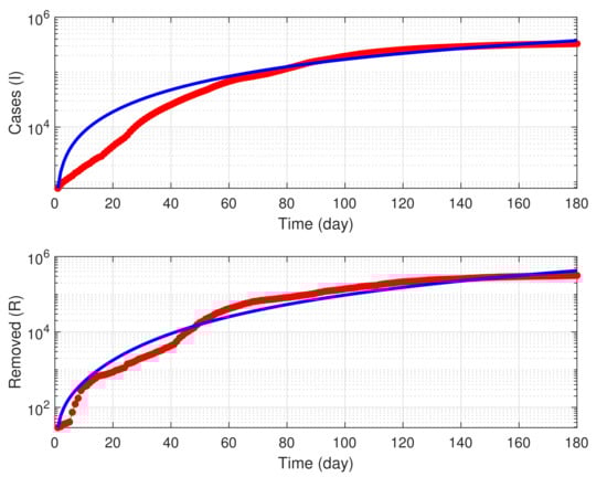
Figure 1. Results of fitting the model to COVID-19 cases in Saudi Arabia for a period of 6 months starting from 24 March 2020. Blue solid line, model predictions; red points, actual data.

Table 2. Model parameters.

Parameter	Definition	Value	Source
b	Dimensionless hospital-bed-to-population ratio	$6.32\times {10}^{-7}$	[21]
$m_1$	Half-saturation of incidence rate	$7.2965\times {10}^5$	fitted
$m_2$	Half-saturation of media effects	$2.8736\times {10}^{-8}$	fitted
${\beta }_2$	Awareness rate	${10}^{-5}$	fitted
${{\gamma }_1}_0$	Minimum recovery rate	0.0026	fitted
${{\gamma }_1}_1$	Maximum recovery rate	0.750	fitted
${\gamma }_2$	Recovery rate of quarantine at home	$7.14\times {10}^{-2}$	[27]
$\mu$	Natural death rate	$4.21\times {10}^{-5}$	[26]
$ϵ$	Quarantine rate	$0.0143$	fitted
$\sigma$	Inverse of mean latent period	0.333	[27]

For bifurcation studies, it is convenient to choose ${\mathcal{R}}_0$ as the main bifurcation parameter. The disease transmission rate ${\beta }_1$ can be derived from Equation (21). Using the obtained fitted values (Table 2), the condition (Equation (39)) for the backward bifurcation to occur is $b<1.308\times {10}^{-6}$. Figure 2a shows the bifurcation diagram for $b=6.32\times {10}^{-7}$, which is the actual dimensionless value of the hospital-bed-to-population ratio. This value was smaller than aforementioned critical value. A limit point (LP) occurred at ${\mathcal{R}}_0=0.6164$, and the diagram also shows a Hopf point at ${\mathcal{R}}_0=0.6165$. An unstable limit cycle branch bifurcated from the subcritical Hopf bifurcation and terminated homoclinically as it collided with the static branch (Figure 2b). The disease-free equilibrium therefore coexisted with the stable endemic solution for any value of ${\mathcal{R}}_0$ between HB $({\mathcal{R}}_0=0.6165)$ and $({\mathcal{R}}_0=1)$. This diagram illustrates the important role the hospital-bed-to-population ratio plays in the disease dynamics. In order for the disease to be suppressed, it is not enough to reduce ${\mathcal{R}}_0$ below unity, but rather to reduce it below the Hopf point. However, it can be seen that the range between the limit point and the Hopf point in terms of ${\mathcal{R}}_0$ was very small (less than ${10}^{-4})$, and therefore, the two points can be considered as one single point.

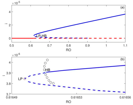
Figure 2. Bifurcation diagram for $b=6.32\times {10}^{-7}$ showing backward bifurcation; solid line, stable branch; dashed line, unstable branch; circles, unstable periodic branches; LP, static limit point; HB, Hopf point.

Figure 3 shows, on the other hand, the continuity diagram if b is increased to $1.4\times {10}^{-6}$, just past the critical value. The backward bifurcation is replaced by a forward bifurcation where the disease-free equilibrium is the only stable outcome for ${\mathcal{R}}_0<1$. The disease is suppressed if the basic reproduction ratio is reduced below unity.

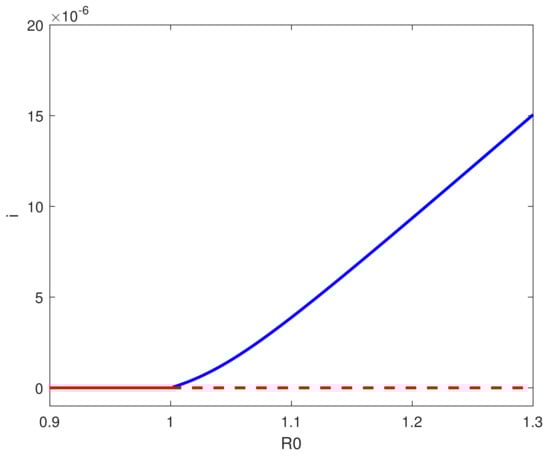
Figure 3. Bifurcation diagram for $b=1.4\times {10}^{-6}$ showing forward bifurcation; solid line, stable branch; dashed line, unstable branch.

Next, we present the results of a sensitivity analysis for the effect of model parameters on the range of the backward bifurcation. There was a necessity to carry out such an analysis since the value of any fitted parameter unavoidably has a degree of error. Our simulations showed that with the exception of the per capita minimum recovery rate (${\gamma }_{10}$), quarantine rate ($ϵ$), and hospital-bed-to-population ratio (b), the change in the value of the Hopf point for all other parameters was extremely small (less than ${10}^{-4}$) even if these parameters were varied over a wide range. Figure 4a shows that the backward bifurcation was attenuated if the minimum recovery rate ${{\gamma }_1}_0$ increased. The value of this parameter is a function of the inherent characteristics of the virus, but it also depends on health resources. Its role can be seen to be important in reducing the backward bifurcation.

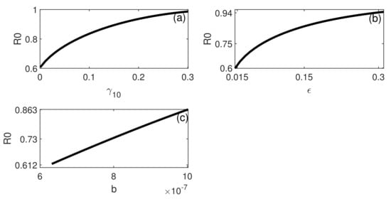
Figure 4. Location of the Hopf point of Figure 2 in terms of the model parameters.

The effect of the quarantine rate is shown in Figure 4b. The Hopf point (and therefore, a backward bifurcation) occurred for a wide range of ${\mathcal{R}}_0$. In fact, increasing the quarantine rate for example from the current fitted value of 0.0143 to 0.25 would increase the Hopf point from 0.6165 to 0.922, and this would substantially decrease the range of the backward bifurcation. This showed the importance of quarantine as a key strategy for the control of the disease.

Finally, it can be seen from Figure 4c that as the dimensionless hospital-bed-to-population ratio (b) increased, the Hopf point occurred at larger values of ${\mathcal{R}}_0$, which means that the backward bifurcation was attenuated.

7. Conclusions

We proposed and analyzed the dynamics of an SEIR model with three modifications: (1) the model considered a quarantined class; (2) the recovery rate was nonlinear and depended on the hospital-bed-to-population ratio; and (3) the model took into account the influence of the media on the public. Most model parameters were obtained by fitting the model to the COVID-19 data in Saudi Arabia. Besides a forward bifurcation, the other behavior encountered in the model was the static coexistence of the endemic equilibrium with the disease-free solution for values of the basic reproduction number between a Hopf point and unity. The paper revealed that the per capita minimum recovery rate, quarantine rate, and hospital-bed-to-population ratio were the most important parameters that could attenuate the backward bifurcation. Public awareness due to the media was found to play a smaller role. However, these results were strictly valid for the country under study and cannot be readily generalized to other countries. The paper was strengthened by the inclusion of a quarantine class, a realistic expression of the recovery rate, and the validation of the model against real data. The model could be strengthened more by the inclusion of more classes such as asymptomatic cases and hospitalized individuals. However, the more structured the model is, the more challenging the data collection and model validation will be. The balance between the quality of fit and the model structure has been made evident in a number of similar studies in Saudi Arabia, where simple SIR models provided better fits than more complex network-based models [29,30].

References

- Anirudh, A. Mathematical modeling and the transmission dynamics in predicting the Covid-19—What next in combating the pandemic. Infect. Dis. Model. 2020, 5, 366–374. [Google Scholar] [CrossRef] [PubMed]
- Cooper, I.; Mondal, A.; Antonopoulos, C.G. A SIR model assumption for the spread of COVID-19 in different communities. Chaos Soliton. Fract. 2020, 139, 110057. [Google Scholar] [CrossRef]
- Koziol, K.; Stanislawski, R.; Bialic, G. Fractional-Order SIR epidemic model for transmission prediction of COVID-19 disease. Appl. Sci. 2020, 10, 8316. [Google Scholar] [CrossRef]
- He, S.; Peng, Y.; Sun, K. SEIR modeling of the COVID-19 and its dynamics. Nonlinear Dyn. 2020, 101, 1667–1680. [Google Scholar] [CrossRef] [PubMed]
- Godio, A.; Pace, F.; Vergnano, A. SEIR Modeling of the Italian Epidemic of SARS-CoV-2 Using Computational Swarm Intelligence. Int. J. Environ. Res. Public Health 2020, 17, 3535. [Google Scholar] [CrossRef] [PubMed]
- Zisad, S.N.; Hossain, M.S.; Hossain, M.S.; Andersson, K. An Integrated Neural Network and SEIR Model to Predict COVID-19. Algorithms 2021, 14, 94. [Google Scholar] [CrossRef]
- Prathumwan, D.; Trachoo, K.; Chaiya, I. Mathematical Modeling for Prediction Dynamics of the Coronavirus Disease 2019 (COVID-19) Pandemic, Quarantine Control Measures. Symmetry 2020, 12, 1404. [Google Scholar] [CrossRef]
- Feng, L.-X.; Jing, S.-L.; Hu, S.-K.; Wang, D.-F. Modelling the effects of media coverage and quarantine on the COVID-19 infections in the UK. Math. Biosci. Eng. 2020, 17, 3618–3636. [Google Scholar] [CrossRef] [PubMed]
- Mohsen, A.A.; Al-Husseiny, H.F.; Zhou, X.; Hattaf, K. Global stability of COVID-19 model involving the quarantine strategy and media coverage effects. AIMS Public Health 2020, 7, 587–605. [Google Scholar] [CrossRef]
- Sardar, T.; Nadim, S.; Rana, S.; Chattopadhyay, J. Assessment of lockdown effect in some states and overall India: A predictive mathematical study on COVID-19 outbreak. Chaos Soliton Fract. 2020, 139, 110078. [Google Scholar] [CrossRef]
- Linka, K.; Peirlinck, M.; Costabal, F.S.; Kuhl, E. Outbreak dynamics of COVID-19 in Europe and the effect of travel restrictions. Comput. Methods Biomech. Biomed. Eng. 2020, 23, 710–717. [Google Scholar] [CrossRef] [PubMed]
- Kwuimy, C.A.K.; Nazari, F.; Jiao, X.; Rohani, P.; Nataraj, C. Nonlinear dynamic analysis of an epidemiological model for COVID 19 including public behavior and government action. Nonlinear Dyn. 2020, 101, 1545–1559. [Google Scholar] [CrossRef] [PubMed]
- Ajbar, A.; Alqahtani, R.T. Bifurcation analysis of a SEIR epidemic system with governmental action and individual reaction. Adv. Differ. Equ. 2020, 2020, 1–14. [Google Scholar] [CrossRef] [PubMed]
- Ghostine, R.; Gharamti, M.; Hassrouny, S.; Hoteit, I. An extended SEIR Model with vaccination for forecasting the COVID-19 pandemic in Saudi Arabia using an ensemble Kalman filter. Mathematics 2021, 9, 636. [Google Scholar] [CrossRef]
- Ruan, S.; Wang, W. Dynamical behavior of an epidemic model with a nonlinear incidence rate. J. Differ. Equ. 2003, 188, 135–163. [Google Scholar] [CrossRef]
- Tang, Y.; Huang, D.; Ruan, S.; Zhang, W. Coexistence of limit cycles and homoclinic loops in a SIRS model with a nonlinear incidence rate. SIAM J. Appl. Math. 2008, 69, 621–639. [Google Scholar] [CrossRef]
- Hu, Z.; Ma, W.; Ruan, S. Analysis of SIR epidemic models with nonlinear incidence rate and treatment. Math. Biosci. 2012, 238, 12–20. [Google Scholar] [CrossRef]
- Wang, W. Backward bifurcation of an epidemic model with treatment. Math. Biosci. 2006, 201, 58–71. [Google Scholar] [CrossRef]
- Chan, C.; Zhu, H. Bifurcations and complex dynamics of an SIR model with the impact of the number of hospital beds. J. Diff. Equ. 2014, 257, 1662–1688. [Google Scholar] [CrossRef]
- Cui, Q.; Qiu, Z.; Liu, W.; Hu, Z. Complex dynamics of an SIR epidemic model with nonlinear saturate incidence and recovery rate. Entropy 2017, 19, 305. [Google Scholar] [CrossRef]
- Saudi Ministry of Health. Available online: https://www.moh.gov.sa/en/Pages/Default.aspx (accessed on 2 November 2020).
- De la Sen, M.; Ibeas, A.; Agarwal, R.P. On Confinement and Quarantine Concerns on an SEIAR Epidemic Model with Simulated Parameterizations for the COVID-19 Pandemic. Symmetry 2020, 12, 1646. [Google Scholar] [CrossRef]
- Corduneanu, C. Principles of Differential and Integral Equations; Allyn and Bacon: Boston, MA, USA, 1971. [Google Scholar]
- Van den Driessche, P.; Watmough, J. Reproduction numbers and subthreshold endemic equilibria for compartmental models of disease transmission. Math. Biosci. 2002, 180, 29–48. [Google Scholar] [CrossRef]
- Castillo-Chavez, C.; Song, B. Dynamical models of tuberculosis and their applications. Math. Biosci. Eng. 2004, 1, 361–404. [Google Scholar] [CrossRef] [PubMed]
- General Authority for Statistics, Saudi Arabia. Available online: https://www.stats.gov.sa/en/5305 (accessed on 2 November 2020).
- Lina, Q.; Zhao, S.; Gao, D.; Lou, Y.; Yang, S.; Musa, S.S.; Wang, M.H.; Cai, Y.; Wang, W.; Yang, L.; et al. A conceptual model for the coronavirus disease 2019 (COVID 19) outbreak in Wuhan, China with individual reaction and governmental action. Int. J. Infect. Dis. 2020, 93, 211–216. [Google Scholar] [CrossRef] [PubMed]
- COVID-19 Dashbard. Available online: https://covid19.moh.gov.sa/ (accessed on 2 November 2020).
- Alharbi, Y.; Alqahtani, A.; Albalawi, O.; Bakouri, M. Epidemiological modeling of COVID-19 in Saudi Arabia: Spread projection, awareness, and impact of treatment. Appl Sci. 2020, 10, 5895. [Google Scholar] [CrossRef]
- Alrasheed, H.; Althnian, A.; Kurdi, H.; Al-Mgren, H.; Alharbi, S. COVID-19 Spread in Saudi Arabia: Modeling, simulation and analysis. Int. J. Environ. Res. Public Health 2020, 17, 7744. [Google Scholar] [CrossRef]
Publisher’s Note: MDPI stays neutral with regard to jurisdictional claims in published maps and institutional affiliations. |
© 2021 by the authors. Licensee MDPI, Basel, Switzerland. This article is an open access article distributed under the terms and conditions of the Creative Commons Attribution (CC BY) license (https://creativecommons.org/licenses/by/4.0/).