Simulation and Analysis of Indoor Air Quality in Florida Using Time Series Regression (TSR) and Artificial Neural Networks (ANN) Models

Abstract

Exposures to air pollutants have been associated with various acute respiratory diseases and detrimental human health. Analysis and further interpretation of air pollutant patterns are correspondingly important as monitoring them. In the present study, the 24-h and four-month indoor and outdoor PM_2.5, PM₁₀, NO₂, relative humidity, and temperature were measured simultaneously for a laboratory in Gainesville city, Florida. The indoor PM_2.5, PM₁₀, and NO₂ concentrations were predicted using multiple linear regression (MLR), time series regression (TSR), and artificial neural networks (ANN) models. The modeling conducted in this study aims to perform a cross comparison study between these models in a symmetric environment. The value of root-mean-square error was improved by 18.33% in comparison with the MLR model. In addition, the value of the coefficient of determination was improved by 24.68%. The ANN model had the best performance and could predict the target air pollutants at 10-min intervals of the studied building with 90% accuracy levels. The TSR model showed slightly better performance compared to the MLR model. These results can be accordingly referred for studies analyzing indoor air quality in similar building types and climate zones.

1. Introduction

Indoor air quality (IAQ) deterioration has been linked to the increased health risk of sick building syndrome (SBS) and building-related illness (BRI) [1,2]. People spend most of their daily lives in indoor environments, even though indoor air pollutant concentrations are on average three to five times higher than outdoors [3,4,5]. The target air pollutants selected in this study were particulate matter (PM_2.5, PM₁₀) and nitrogen dioxide (NO₂). They are the most common indoor air pollutants defined in both the United States Environmental Protection Agency (US EPA) and the World Health Organization (WHO) standards [6,7,8]. Fine particle matter is mainly generated from incomplete combustion, vehicle emissions, and dust [1,6,9]. The most common source of reddish-brown gas (NO₂) is the combustion of fossil fuel [1,6,10,11]. Effective analysis and prediction of indoor air pollutant patterns are correspondingly critical as monitoring them.

In recent years, laser-based semiconductor techniques and low-cost air pollution monitoring techniques have rapidly surged [12,13,14]. There has been growing interest in determining the relationships between indoor and outdoor air quality using real-time measured data. Various prediction models have been developed to predict the IAQ based on environmental parameters. For example, Hassanvand et al. [15] and Chithra et al. [16] developed linear regression models to study and forecast the mass concentrations of indoor and outdoor particulate matter (PM₁₀, PM_2.5, and PM₁) in a residential house and a school building, respectively. Mohammadyan et al. [17] applied multiple regression models using indoor and outdoor environmental data (fine particles, temperature, and relative humidity). The model performed moderately predictive for the measured indoor pollutants. Jafta et al. [18] developed leave-one-out cross-validation-based multivariate models using PM_2.5 concentrations, meteorological information, and household human activities as inputs, while Shupler et al. [19] added housing material, season as one of the inputs. Kim et al. [20] used principal component analysis (PCA)-based linear models to predict indoor particulate matter (PM) by performing dimension reduction. Tong et al. [21] reported that the linear mixed-effects regression model showed moderately predictive for indoor PM_2.5, and the fitted model resulted that outdoor PM_2.5, relative humidity, and indoor PM_2.5 were positively associated. Yuchi et al. [22] and Lin et al. [23] reported that random forest-based machine learning predictive models and multiple linear regression models showed similar performance when predicting levels of certain indoor pollutants. Previous literature review reveals that most studies predicting indoor air quality focused on outdoor concentrations and human behaviors. Although most of the measured data are ordered by time, and many observations showed potential time delay between outdoor pollutants leak and the indoor concentrations [24,25,26,27]. However, to our knowledge, no study of relationships between indoor and outdoor air quality has attempted to include time-delay effects within the variables in regression analysis. Besides, artificial neural networks (ANN) have gained attention by a few researchers in recent years for indoor air quality forecasting [28,29,30,31,32,33]. Park et al. [25], Challoner et al. [34], and Saad et al. [35] reported that ANN-predicted indoor pollutant concentrations showed better performance than other regression models. Conversely, Liu et al. [31] developed nonlinear regression models that predicted IAQ levels showed higher performance over other prediction models (partial least squares, backpropagation ANN, and least-squares).

This study performed numerical simulations with monitored indoor and outdoor environmental data, coupled with the multiple linear regression model, the time series regression model, and the ANN-based model, to determine the relationships between indoor and outdoor air quality. Furthermore, these models are expected to predict the indoor air pollutant concentrations in a laboratory building in Florida. The objective of this paper is to perform a cross comparison study between multiple linear regression (MLR), time series regression (TSR), and non-linear ANN models. The hypothesis of this study is that the real-time monitored air quality data can fit better under non-linear models such as ANN compared to linear prediction models. The outline of this paper is as follows. In Section 2, the sampling protocols and methods of TSR and ANN are introduced. In Section 3, results of a cross-comparison of the aforementioned models are presented. The final section addresses the conclusion of this article.

2. Materials and Methods

2.1. Sampling Site and Sampling Protocol

The measurement of the test building was conducted between 17 May 2020 (Sunday) and 18 September 2020 (Friday) in Gainesville city, Florida, United States. The building chosen for air quality monitoring is mechanically conditioned throughout the year, and the windows are closed to meet the American Society of Heating, Refrigerating, and Air-Conditioning Engineers (ASHRAE) Standard 62.1-2019 [36]. The laboratory building mainly functions as an office space with a 321 sq. ft floor area coupled with a single ducted air handling unit, which can provide a PM_2.5 removal efficiency of 25% [37]. The standardized US EPA protocol for characterizing IAQ in large office buildings is followed to reduce measurement uncertainty [12,38]. A four-month indoor and outdoor air quality measurement was carried out with 10 min sampling intervals for 24 h continuously. Two US EPA (Air Quality Sensor Performance Evaluation Center) qualified monitors (Air Quality Egg, Version-2018) were used to measure the concentration of indoor and outdoor PM_2.5, PM₁₀, and NO₂, as well as relative humidity and temperature (RHT) [11,39,40]. The basic specifications of the monitor are shown in Table 1. The indoor monitor was placed about 3.6 feet above the floor, 1.5 feet away from an interior wall. Outdoor measurement was conducted simultaneously with indoors. A weatherproofed monitor was set up 5 feet above the surface of the deck outside the room (Figure 1).

Table 1. Specifications of the selected sensor modules.

Measured Parameter	Product	Manufacturer	Measurement Tolerance	Measuring Range
PM2.5, PM10	PMS5003	Plantower	±10% or 100~500 μg/m3;	0~500 µg/m3, ≥1000 µg/m3
NO2	3SP_NO2_5FP	SPEC	±5% or 10 ppb	0~5 ppm
CO	3SP_CO_1000	SPEC	±2%	0 to 1000 ppm
RHT	DHT22	Aosong Electronic	±0.5 °C and ±1%	−40 °F to 176 °F, 0% to 100%

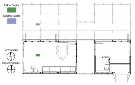
Figure 1. Floor plan of the sampling building.

2.2. Multiple Linear Regression Model

The monitored data are extracted and subjected to descriptive statistics such as mean, standard deviation, indoor/outdoor ratio (I/O), and variance using Anaconda Python and Jupyter Notebooks [41]. Multiple linear regressions were performed to assess and predict the relationship between indoor air pollutants (PM_2.5, PM₁₀, and NO₂) and other measured environmental parameters. A multiple linear regression model can be expressed as Equation (1) [22,42,43]:

$$Y_{in}={\beta }_0+{\beta }_1{x}_1+{\beta }_2{x}_2+{\beta }_3{x}_3+\cdots +{\beta }_{p-1}{x}_{p-1}+\epsilon$$

(1)

where $Y_{in}$ is the dependent variable, $\beta =({\beta }_0, {\beta }_1,\dots , {\beta }_{p-1})$ are regression coefficients, $x=\left(x_1, x_2,\dots x_{p-1}\right)$ are the independent variables, and $\epsilon$ is the random error term. The performance of developed MLR models was examined by calculating the coefficient of determination (R²), and root means square error (RMSE). The performance indicators were calculated as Equations (2) and (3) [44,45,46]:

$${\mathrm{R}}^2=\frac{{{\displaystyle \sum }}_{\mathrm{i}}^{\mathrm{n}}{\left({\hat{\mathrm{y}}}_{\mathrm{i}}-{\overline{\mathrm{y}}}_{\mathrm{i}}\right)}^2}{{{\displaystyle \sum }}_{\mathrm{i}}^{\mathrm{n}}{\left({\mathrm{y}}_{\mathrm{i}}-\overline{\mathrm{y}}\right)}^2}$$

(2)

$$\mathrm{RMSE}=\sqrt{\frac{{{\displaystyle \sum }}_{\mathrm{i}}^{\mathrm{n}}{\left({\hat{\mathrm{y}}}_{\mathrm{i}}-{\mathrm{y}}_{\mathrm{i}}\right)}^2}{\mathrm{n}}}$$

(3)

where i is the prediction variable at present while ${\hat{\mathrm{y}}}_{\mathrm{i}}$ is the predicted value at each time, ${\mathrm{y}}_{\mathrm{i}}$ is the measured NO₂ (PM_2.5 or PM₁₀) concentration, $\overline{\mathrm{y}}$ is the average value of measured NO₂ (PM_2.5 or PM₁₀) concentrations.

2.3. Time Series Regression Model

To predict the dependency between recorded variables when considering time-lag and time-accumulation effects, the TSR models were developed using MATLAB R2020a [47,48]. The autoregressive (AR) approaches were implemented for forecasting based on the same datasets used in the MLR models [49,50]. In an AR method, each variable is a linear function of the past values of itself and other previously recorded values [50,51,52]. The inputs of the model were the indoor and outdoor levels of temperature (°F), relative humidity (%), PM_2.5 (µg/m³), PM₁₀ (µg/m³), and NO₂ (ppb). The indoor PM_2.5, PM_10, or NO₂ of the laboratory building was considered as the output. The input variables were then slowly increased by adding the target pollutant of previous minutes (10 min intervals) to find the best-fit model (See Figure 2). To evaluate the performance of the TSR models and avoid the biased estimation, we computed RMSE between simulated and real-time measured data [29,44].

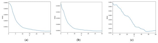
Figure 2. RMSE of tested models (RMSE = y-axis, data measurements—‘k’ = x-axis): (a) Indoor_PM_2.5, (b) Indoor_PM₁₀, (c) Indoor_NO₂.

From Figure 2a,b, the best results were found by the implementation of the past 250 min observed value of indoor PM_2.5 and indoor PM₁₀, respectively. Figure 2c shows the best results were found by the implementation of the past 470 min observed value of indoor NO₂. The following are the obtained equations for the TSR model [49,50]:

$$\begin{array}{c}{\mathrm{PM}}_{2.5\_\mathrm{in}}={\displaystyle {\displaystyle \sum }_{k=0}^{\mathrm{K}}}{\mathrm{a}}_{\mathrm{k}}{\mathrm{PM}}_{2.5\_\mathrm{out}}\left(\mathrm{t}-\mathrm{k}\right)+{\mathrm{bT}}_{\mathrm{out}}\left(\mathrm{t}\right)+{\mathrm{cH}}_{\mathrm{out}}\left(\mathrm{t}\right)+{\mathrm{dPM}}_{10\_\mathrm{out}}\left(\mathrm{t}\right)+{\mathrm{eNO}}_{2\_\mathrm{out}}\left(\mathrm{t}\right)+{ \mathrm{fT}}_{\mathrm{in}}\left(\mathrm{t}\right)+{\mathrm{gH}}_{\mathrm{in}}\left(\mathrm{t}\right)\\ +{\mathrm{hPM}}_{10\_\mathrm{in}}\left(\mathrm{t}\right)+{\mathrm{iNO}}_{2\_\mathrm{in}}\left(\mathrm{t}\right)+ \mathrm{j}\end{array}$$

(4)

$$\begin{array}{c}{\mathrm{PM}}_{{10}_{\_\mathrm{in}}}={\displaystyle {\displaystyle \sum }_{k=0}^{\mathrm{K}}}{\mathrm{a}}_{\mathrm{k}}{\mathrm{PM}}_{10\_\mathrm{out}}\left(\mathrm{t}-\mathrm{k}\right)+{\mathrm{bT}}_{\mathrm{out}}\left(\mathrm{t}\right)+{\mathrm{cH}}_{\mathrm{out}}\left(\mathrm{t}\right)+{\mathrm{dPM}}_{2.5\_\mathrm{out}}\left(\mathrm{t}\right)+{\mathrm{eNO}}_{2\_\mathrm{out}}\left(\mathrm{t}\right)+{\mathrm{fT}}_{\mathrm{in}}\left(\mathrm{t}\right)+{\mathrm{gH}}_{\mathrm{in}}\left(\mathrm{t}\right)\\ +{\mathrm{hPM}}_{2.5\_\mathrm{in}}\left(\mathrm{t}\right)+{\mathrm{iNO}}_{2\_\mathrm{in}}\left(\mathrm{t}\right)+\mathrm{j}\end{array}$$

(5)

$$\begin{array}{c}{\mathrm{NO}}_{2\_\mathrm{in}}={\displaystyle {\displaystyle \sum }_{k=0}^{\mathrm{K}}}{\mathrm{a}}_{\mathrm{k}}{\mathrm{NO}}_{2\_\mathrm{out}}\left(\mathrm{t}-\mathrm{k}\right)+{\mathrm{bT}}_{\mathrm{out}}\left(\mathrm{t}\right)+{\mathrm{cH}}_{\mathrm{out}}\left(\mathrm{t}\right)+{\mathrm{dPM}}_{2.5\_\mathrm{out}}\left(\mathrm{t}\right)+{\mathrm{ePM}}_{10\_\mathrm{out}}\left(\mathrm{t}\right)+{\mathrm{fT}}_{\mathrm{in}}\left(\mathrm{t}\right)\\ +{\mathrm{gH}}_{\mathrm{in}}\left(\mathrm{t}\right)+{\mathrm{hPM}}_{2.5\_\mathrm{in}}\left(\mathrm{t}\right)+{\mathrm{iPM}}_{10\_\mathrm{in}}\left(\mathrm{t}\right)+\mathrm{j}\end{array}$$

(6)

where $\mathrm{a},\mathrm{b},\mathrm{c},\mathrm{d},\mathrm{e},\mathrm{f},\mathrm{g},\mathrm{h}, \mathrm{i}, \mathrm{and} \mathrm{j}$ are the coefficient. k is the number of time intervals (10 min). ${\mathrm{T}}_{\mathrm{out}}\left(\mathrm{t}\right){ \mathrm{and} \mathrm{T}}_{\mathrm{in}}\left(\mathrm{t}\right)$ are the outdoor and indoor temperature measured at time t, respectively. ${\mathrm{H}}_{\mathrm{out}}\left(\mathrm{t}\right){ \mathrm{and} \mathrm{H}}_{\mathrm{in}}\left(\mathrm{t}\right)$ represent the outdoor and indoor relative humidity at time t. ${\mathrm{PM}}_{2.5\_\mathrm{out}}\left(\mathrm{t}\right),{ \mathrm{PM}}_{10\_\mathrm{out}}\left(\mathrm{t}\right),{ \mathrm{PM}}_{2.5\_\mathrm{in}}\left(\mathrm{t}\right),{ \mathrm{and} \mathrm{PM}}_{10\_\mathrm{in}}\left(\mathrm{t}\right)$ are the measured values of outdoor and indoor PM_2.5 and PM₁₀ at time t. ${\mathrm{NO}}_{2\_\mathrm{out}}\left(\mathrm{t}\right){\mathrm{and} \mathrm{NO}}_{2\_\mathrm{in}}\left(\mathrm{t}\right)$ represent the outdoor and indoor calibration of ${\mathrm{NO}}_2$(pbb) at time t.

2.4. Artificial Neural Networks Model

Artificial neural networks have been widely employed to investigate complex ambient-air processes. Many studies have predicted the concentrations of indoor air pollutants with ANN [33,35,46]. Multi-layer perceptron (MLP) network is one of the major types of ANN architectures [53]. Usually, the MLP network is consists of input, output, and multi-layers (including a hidden layer) [54]. Each layer is composed of several interconnected non-linear processing components called neurons or nodes [29,32]. The selected neurons were connected to other neurons in adjacent layers through adaptive synaptic coefficients [29,54]. In this study, two-layer feed-forward neural network models were developed using the neural network toolbox of MATLAB R2020a [48]. The same dataset used in the MLR and TSR approach, 18,144 time-series data for each input neuron used to train the ANN models. The logistic sigmoid transfer function and linear activation function were used to avoid the fitting problem between input and output datasets. The input dataset was normalized using min–max normalization. The ANN models were trained with the Levenberg–Marquardt (LM) based back-propagation (BP) algorithm [44,52,55]. The LM algorithm is one of the most effective algorithms which accelerates the convergence rate of the ANN with multilayer perceptron (MLP) architectures and reserves computational resources [35,46]. Studies have found the optimal number of hidden neurons to obtain the best network performance. In this study, the number of hidden layers was computed to be 10 from several iterations [52,54,55,56,57]. As shown in Figure 3, the input layer contains nine neurons of indoor and outdoor air quality parameters. The measured indoor concentrations of PM_2.5, PM₁₀, and NO₂ were considered as the desired target of the ANN models. For each training, the database was randomized into three groups: 70% training, 15% validation, and 15% testing [32,54]. The optimum network architecture of the ANN models was developed with 10 hidden layers [52,56]. The performance of developed ANN models was examined by calculating the coefficient of determination (R²) and root means square error (RMSE) [44,46].

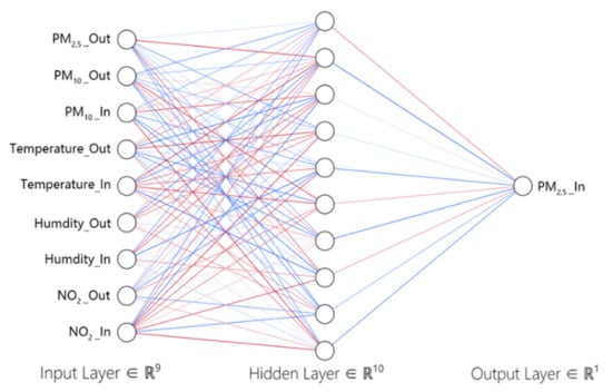
Figure 3. A schematic structure of a two-layer feed-forward network used in this study.

3. Results and Discussion

3.1. Measured Environmental Parameters

The descriptive statistics of measured indoor and outdoor environmental data are presented in Table 2 and Figure 4. The mean indoor and outdoor temperatures were 70.7 °F and 81.5 °F, respectively, while outdoor relative humidity had a slightly higher mean and a larger standard deviation than indoors. The average mean of indoor PM_2.5, PM₁₀, and NO₂ was significantly lower indoors than outdoors. It shows that the indoor concentration of PM_2.5 range was 0 μg/m³ to 38.5 μg/m³, indoor PM₁₀ was 0 μg/m³ to 68 μg/m³, and NO₂ was 72.3 ppb to 83.9 ppb. Figure 5 shows the plots of the four-month-long continuous records based on 10 min intervals. Most indoor PM_2.5 and PM₁₀ data met the 24 h safe levels in ASHRAE 62.1-2019 standard [36]. The indoor concentrations of both particulate matters followed a similar diurnal pattern as the outdoor concentrations. It can be seen from Figure 4c. The indoor NO₂ data show a significantly stable pattern than the outdoors across the sampling period. The potential reasons for this trend might be due to most gaseous pollutants have infiltrated and a lack of indoor NO₂ sources [1,12,58]. However, the majority of indoor NO₂ data lie above the annual requirements of ASHRAE 62.1 standard (53 ppb) [11,36].

Table 2. Descriptive statistics of indoor environmental parameters.

	Indoor				Outdoor				I/O Ratio
Environmental Parameters	Average ± SD	Min	Max	Median	Average ± SD	Min	Max	Median	Mean
PM2.5 (µg/m3)	2.29 ± 2.27	0	38.5	1.70	7.20 ± 4.35	0	68.0	6.40	0.33
PM10 (µg/m3)	2.40 ± 2.37	0	45.0	1.80	8.06 ± 4.74	0	77.6	7.20	0.31
NO2 (ppb)	60.9 ± 7.35	30.7	133	61.9	132 ± 68.7	0	876	141	1.34
Temperature (°F)	75.0 ± 1.22	72.3	83.9	74.8	81.5 ± 7.70	65.0	106	79.7	1.03
Relative Humidity (%)	70.7 ± 3.90	50.9	82.1	71.5	71.1 ± 14.1	27.8	90.3	75.4	0.92

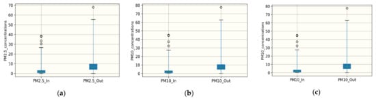
Figure 4. Box plots of air pollutant concentrations: (a) PM_2.5, (b) PM₁₀, (c) NO₂.

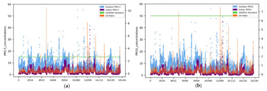
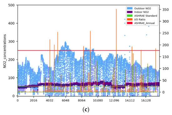
Figure 5. Four-month evaluation of indoor and outdoor air quality measured at 10 min intervals (2016 observational points for two weeks equating to 18144): (a) PM_2.5, (b) PM₁₀, (c) NO₂.

3.2. Correlation between Indoor and Outdoor Data

Simple linear regression and the nonlinear Spearman’s rank correlation were performed to extract the direct correlation between indoor data and their corresponding outdoor data. The dataset was also used to investigate the symmetry among indoor and outdoor time-series concentrations. The input dataset was normalized using standardized normalization. Figure 6a,b show the linear correlation and symmetric distributions between indoor and outdoor particulate matters (PM_2.5 and PM₁₀) with very coefficient of determination (R²__PM2.5 = 0.26; R²__PM10 = 0.24, p < 0.01). However, statistically moderate correlation (R__PM2.5 = 0.53; R__PM10 = 0.52) were found in the Spearman’s rank results. From Figure 7, Spearman’s coefficient shows a significant correlation coefficient (R__NO2 = 0.87) between indoor and outdoor NO₂. Conversely, a very low correlation was found between indoor and outdoor NO₂ in the linear regression analysis (Figure 6c). There were statistically significant mismatches between the non-linear Spearman’s coefficients and the linear correlation coefficients. The results also indicated that the univariate linear regression method might not accurately predict the indoor concentrations of PM_2.5, PM₁₀, and NO₂. Since these results are not compelling, multivariate analysis and further validation should be considered for the IAQ prediction model.

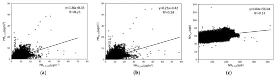
Figure 6. Comparison between indoor and outdoor data in using linear regression: (a) PM_2.5, (b) PM₁₀, (c) NO₂.

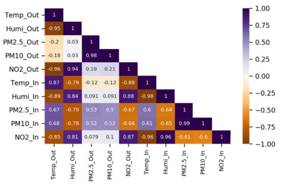
Figure 7. Spearman correlation heat map for indoor and outdoor environmental parameters.

3.3. Cross-Comparison of the MLR, TSR, and ANN Models in the Prediction of the Indoor PM_2.5 and PM₁₀

The developed TSR and ANN models were used to simulate the 10 min average indoor particulate matter concentrations (PM_2.5 and PM₁₀) of a laboratory building near downtown Gainesville city, Florida. To better evaluate the prediction performance of each model, their output results were compared to the results of conventional multiple linear regression (MLR). Figure 8 shows the original and simulated indoor PM_2.5 by the time-series and developed models for the period of 17 May 2020 to 18 September 2020. It can be observed that the MLR, TSR, and ANN models can successfully predict the indoor PM_2.5 concentrations and their trend. The adjusted p-values which are less than 0.001 were validated by using F-test. From the simulated data, the R² values of the models (MLR, TSR, ANN) are above 0.9 (p < 0.001), and their MRSE values are less than 0.1 (p < 0.001) (Table 3). TSR and MLR had the same R² values, but the RMSE value of TSR was 1.31% less than that of MLR. Additionally, the R² value of the ANN model was found to be 0.08% higher than the MLR model, and the RMSE of ANN was lower than the MLR by 5.37%. Similar performance was observed in the case of indoor PM₁₀ (Figure 9). MLR (R² = 0.9985, p < 0.001), TSR (R² = 0.9986, p < 0.001), ANN (R² = 0.9995, p < 0.001) all successfully predicted indoor PM10 concentrations. The RMSE of the TSR model was lower than the MLR by 1.02%. The R² value of the ANN model was 0.09% higher than the MLR, and the RMSE of ANN was 13.66% lower than the MLR. In summary, the ANN models had the best performance among all the models to predict indoor particulate matters (PM_2.5 and PM₁₀), and the TSR models had better performance than the MLR. A random forest-based ANN in a residential environment studying indoor PM_2.5 concentrations found with R² value and cross-validation R² values of 0.93 and 0.65, respectively [59]. Park et al. [25] also conducted an ANN study in which the average value of indoor PM₁₀ concentration had an average value of 0.62 and mean RMSE of 33.04 in Seoul metropolitan subway stations. These studies had different environmental conditions which might have caused alternate results compared to our study. Besides, several studies have proved that factors, such as building materials, indoor environment conditions, human activities, and others, may contribute to the indoor particulate matter concentrations [57,60,61,62,63,64].

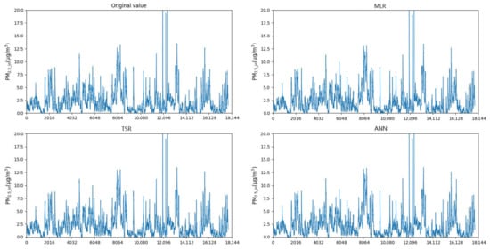
Figure 8. Simulated indoor PM_2.5 concentrations at 10 min intervals (2016 observational points for two weeks equating to 18144).

Table 3. Summary of the prediction models for indoor PM_2.5 and PM₁₀.

	Indoor PM2.5				Indoor PM10
	R2	RMSE	Changes		R2	RMSE	Changes
			R2	RMSE			R2	RMSE
MLR	0.9986	0.0862	-	-	0.9985	0.0906	-	-
TSR	0.9986	0.0851	0	−1.31%	0.9986	0.0897	0	−1.02%
ANN	0.9994	0.0816	0.08%	−5.37%	0.9995	0.0782	0.09%	−13.66%

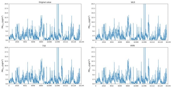
Figure 9. Simulated indoor PM₁₀ concentrations at 10 min intervals (2016 observational points for two weeks equating to 18144).

3.4. Cross-Comparison of the MLR, TSR, and ANN Models in Prediction of the Indoor NO₂

The predicted results of the developed models for indoor NO₂ concentrations are illustrated in Figure 10 and Table 4. The adjusted p-values which are less than 0.001 were validated by using F-test. The validation of each developed model using 15% of the dataset showed that the R² (p < 0.001) value of models were 0.7230 (MLR), 0.7233 (TSR), and 0.9014 (ANN), while the RMSEs (p < 0.001) were 3.8861, 3.8558, and 3.1737, respectively, indicating that the models successfully predicted indoor NO₂ concentrations. The reason RMSE is higher in NO₂ prediction models than particulate matter models can be ascribed to the high spatial variation for NO₂ concentrations in the outdoor environment. However, again the ANN model shows the best performance in predicting the indoor NO₂ levels comparing to the TSR and MLR. The R² value (p < 0.001) of the ANN model was found to be 24.68% higher than the MLR model, and the RMSE (p < 0.001) of ANN was lower than the MLR by 18.33%. The TSR model gave slightly better performance compared to the MLR model. A study in an office room in a commercial building in Dublin showed that the prediction ability of R2 was 0.899 through ANN model compared to 0.11 through linear regression model [34].

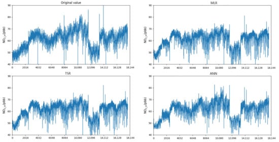
Figure 10. Simulated indoor NO₂ concentrations at 10-min intervals (2016 observational points for two weeks equating to 18144).

Table 4. Summary of the prediction models for indoor NO₂.

Indoor NO2
	R2	RMSE	Changes
			R2	RMSE
MLR	0.7230	3.8861	-	-
TSR	0.7233	3.8558	0.05%	−0.78%
ANN	0.9014	3.1737	24.68%	−18.33%

4. Conclusions

The study measured the time-series data of concentrations of air pollutants (PM_2.5, PM₁₀, and NO₂), as well as temperature and relative humidity for both indoor and outdoor of a research lab, for a duration of four months in the midst of the COVID-19 pandemic (Supplementary Materials). The real-time measured data were used to develop predictive models to analyze the relationship between pollutant concentrations along with its symmetry. The hypothesis was verified using the abovementioned predictive models. In addition, the results showed that there was a complex non-linear relationship between indoor and outdoor environmental parameters. Indoor air quality (PM_2.5, PM₁₀, and NO₂) can be accurately estimated by the MLR, TSR, and ANN models. The comparison results showed that the ANN model had the best performance and could predict the PM_2.5 and PM₁₀ at 10 min intervals of the studied building with 90% accuracy levels. The TSR model had a similar performance with the MLR model when considering the time delay between indoor and corresponding outdoor air pollutants. In case of indoor PM_2.5 and PM₁₀ prediction, the R² values under the MLR models were more than 0.95 (p < 0.01) and the RMSE values were less than 0.1 (p < 0.01). In comparison, ANN model prediction performance was better than the TSR model resulting in an increase in R² value by 0.09% and decrease in RMSE value by 13.66%. In the case of indoor NO₂ prediction, the mean R² value under the MLR model was more than 0.7 (p < 0.01) and the RMSE value was less than 4. In comparison, ANN model prediction performance was better than the TSR model resulting in an increase in R² value by 24.68% (p < 0.01) and decrease in RMSE value by 18.33%. The results in this study indicated that ANN should be predominantly used compared to linear regression models for future research involving time-symmetric environmental parameters. This study can be accordingly referred by building managers to make dynamic adjustments to indoor air quality in similar building types and climate zones. However, the accuracy of the prediction may be influenced by other uncertain parameters such as building type and indoor human activities. The building parameters can be included in the ANN model analyses for better understanding of the relationships between indoor and outdoor air quality.

References

- Ahmed Abdul-Wahab, S.A.; En, S.C.F.; Elkamel, A.; Ahmadi, L.; Yetilmezsoy, K. A review of standards and guidelines set by international bodies for the parameters of indoor air quality. Atmos. Pollut. Res. 2015, 6, 751–767. [Google Scholar] [CrossRef]
- Saeki, Y.; Kadonosono, K.; Uchio, E. Clinical and allergological analysis of ocular manifestations of sick building syndrome. Clin. Ophthalmol. 2017, 11, 517–522. [Google Scholar] [CrossRef][Green Version]
- Raysoni, A.U.; Stock, T.H.; Sarnat, J.A.; Chavez, M.C.; Sarnat, S.E.; Montoya, T.; Holguin, F.; Li, W.-W. Evaluation of VOC concentrations in indoor and outdoor microenvironments at near-road schools. Environ. Pollut. 2017, 231, 681–693. [Google Scholar] [CrossRef]
- Verriele, M.; Schoemaecker, C.; Hanoune, B.; Leclerc, N.; Germain, S.; Gaudion, V.; Locoge, N. The MERMAID study: Indoor and outdoor average pollutant concentrations in 10 low-energy school buildings in France. Indoor Air 2016, 26, 702–713. [Google Scholar] [CrossRef] [PubMed]
- WHO. World Health Statistics 2020: Monitoring Health for the SDGs, Sustainable Development Goals. Available online: https://www.who.int/publications/i/item/9789240005105 (accessed on 27 February 2021).
- NAAQS. Primary National Ambient Air Quality Standards (NAAQS) for Nitrogen Dioxide. Available online: https://www.epa.gov/no2-pollution/primary-national-ambient-air-quality-standards-naaqs-nitrogen-dioxide (accessed on 26 July 2019).
- US-EPA. Report on the Environment, What Are the Trends in Indoor Air Quality and their Effects on Human Health? Available online: https://www.epa.gov/report-environment/indoor-air-quality (accessed on 3 November 2020).
- WHO. Ambient Air Pollution Attributable Death Rate (per 100 000 Population). Available online: https://www.who.int/data/gho/data/indicators/indicator-details/GHO/ambient-air-pollution-attributable-death-rate-(per-100-000-population) (accessed on 26 February 2021).
- Song, P.; Wanga, L.; Hui, Y.; Li, R. PM2.5 Concentrations Indoors and Outdoors in Heavy Air Pollution Days in Winter. Procedia Eng. 2015, 121, 1902–1906. [Google Scholar] [CrossRef]
- Challoner, A.; Gill, L. Indoor/outdoor air pollution relationships in ten commercial buildings: PM2.5 and NO2. Build. Environ. 2014, 80, 159–173. [Google Scholar] [CrossRef]
- Zhang, H.; Srinivasan, R. A systematic review of air quality sensors, guidelines, and measurement studies for indoor air quality management. Sustainability 2020, 12, 9045. [Google Scholar] [CrossRef]
- Zhang, H.; Srinivasan, R.; Ganesan, V. Low cost, multi-pollutant sensing system using raspberry pi for indoor air quality monitoring. Sustainability 2021, 13, 370. [Google Scholar] [CrossRef]
- Yi, W.Y.; Lo, K.M.; Mak, T.; Leung, K.S.; Leung, Y.; Meng, M.L. A Survey of Wireless Sensor Network Based Air Pollution Monitoring Systems. Sensors 2015, 15, 31392–31427. [Google Scholar] [CrossRef] [PubMed]
- Castell, N.; Dauge, F.R.; Schneider, P.; Vogt, M.; Lerner, U.; Fishbain, B.; Broday, D.; Bartonova, A. Can commercial low-cost sensor platforms contribute to air quality monitoring and exposure estimates? Environ. Int. 2017, 99, 293–302. [Google Scholar] [CrossRef] [PubMed]
- Hassanvand, M.S.; Naddafi, K.; Faridi, S.; Arhami, M.; Nabizadeh, R.; Sowlat, M.H.; Pourpak, Z.; Rastkari, N.; Momeniha, F.; Kashani, H.; et al. Indoor/outdoor relationships of PM10, PM2.5, and PM1 mass concentrations and their water-soluble ions in a retirement home and a school dormitory. Atmos. Environ. 2014, 82, 375–382. [Google Scholar] [CrossRef]
- Chithra, V.S.; Shiva Nagendra, S.M. Impact of outdoor meteorology on indoor PM10, PM2.5 and PM1 concentrations in a naturally ventilated classroom. Urban Clim. 2014, 10, 77–91. [Google Scholar] [CrossRef]
- Mohammadyan, M.; Alizadeh-Larimi, A.; Etemadinejad, S.; Latif, M.T.; Heibati, B.; Yetilmezsoy, K.; Abdul-Wahab, S.A.; Dadvand, P. Particulate air pollution at schools: Indoor-outdoor relationship and determinants of indoor concentrations. Aerosol Air Qual. Res. 2017, 17, 857–864. [Google Scholar] [CrossRef]
- Jafta, N.; Barregard, L.; Jeena, P.M.; Naidoo, R.N. Indoor air quality of low and middle income urban households in Durban, South Africa. Environ. Res. 2017, 156, 47–56. [Google Scholar] [CrossRef] [PubMed]
- Shupler, M.; Godwin, W.; Frostad, J.; Gustafson, P.; Arku, R.E.; Brauer, M. Global estimation of exposure to fine particulate matter (PM2.5) from household air pollution. Environ. Int. 2018, 120, 354–363. [Google Scholar] [CrossRef]
- Kim, M.; Sankararao, B.; Kang, O.; Kim, J.; Yoo, C. Monitoring and prediction of indoor air quality (IAQ) in subway or metro systems using season dependent models. Energy Build. 2012, 46, 48–55. [Google Scholar] [CrossRef]
- Tong, X.; Ho, J.M.W.; Li, Z.; Lui, K.H.; Kwok, T.C.Y.; Tsoi, K.K.F.; Ho, K.F. Prediction model for air particulate matter levels in the households of elderly individuals in Hong Kong. Sci. Total Environ. 2020, 717, 135323. [Google Scholar] [CrossRef] [PubMed]
- Yuchi, W.; Gombojav, E.; Boldbaatar, B.; Galsuren, J.; Enkhmaa, S.; Beejin, B.; Naidan, G.; Ochir, C.; Legtseg, B.; Byambaa, T.; et al. Evaluation of random forest regression and multiple linear regression for predicting indoor fine particulate matter concentrations in a highly polluted city. Environ. Pollut. 2019, 245, 746–753. [Google Scholar] [CrossRef] [PubMed]
- Lin, B.; Huangfu, Y.; Lima, N.; Jobson, B.; Kirk, M.; O’Keeffe, P.; Pressley, S.N.; Walden, V.; Lamb, B.; Cook, D.J. Analyzing the relationship between human behavior and indoor air quality. J. Sens. Actuator Netw. 2017, 6, 13. [Google Scholar] [CrossRef]
- Chao, C.Y.; Wong, K.K. Residential indoor PM10 and PM2.5 in Hong Kong and the elemental composition. Atmos. Environ. 2002, 36, 265–277. [Google Scholar] [CrossRef]
- Park, S.; Kim, M.; Kim, M.; Namgung, H.G.; Kim, K.T.; Cho, K.H.; Kwon, S.B. Predicting PM10 concentration in Seoul metropolitan subway stations using artificial neural network (ANN). J. Hazard. Mater. 2018, 341, 75–82. [Google Scholar] [CrossRef]
- Goyal, R.; Khare, M. Indoor-outdoor concentrations of RSPM in classroom of a naturally ventilated school building near an urban traffic roadway. Atmos. Environ. 2009, 43, 6026–6038. [Google Scholar] [CrossRef]
- Deng, G.; Li, Z.; Wang, Z.; Gao, J.; Xu, Z.; Li, J.; Wang, Z. Indoor/outdoor relationship of PM2.5 concentration in typical buildings with and without air cleaning in Beijing. Indoor Built Environ. 2015, 26, 60–68. [Google Scholar] [CrossRef]
- Spinelle, L.; Gerboles, M.; Villani, M.G.; Aleixandre, M.; Bonavitacola, F. Field calibration of a cluster of low-cost commercially available sensors for air quality monitoring. Part B: NO, CO and CO2. Sens. Actuators B Chem. 2017, 238, 706–715. [Google Scholar] [CrossRef]
- Maleki, H.; Sorooshian, A.; Goudarzi, G.; Baboli, Z.; Tahmasebi Birgani, Y.; Rahmati, M. Air pollution prediction by using an artificial neural network model. Clean Technol. Environ. Policy 2019, 21, 1341–1352. [Google Scholar] [CrossRef] [PubMed]
- De Vito, S.; Piga, M.; Martinotto, L.; Di Francia, G. CO, NO2 and NOx urban pollution monitoring with on-field calibrated electronic nose by automatic bayesian regularization. Sens. Actuators B Chem. 2009, 143, 182–191. [Google Scholar] [CrossRef]
- Liu, H.; Yang, C.; Huang, M.; Wang, D.; Yoo, C.K. Modeling of subway indoor air quality using Gaussian process regression. J. Hazard. Mater. 2018, 359, 266–273. [Google Scholar] [CrossRef]
- Rahman, N.H.A.; Lee, M.H.; Suhartono; Latif, M.T. Artificial neural networks and fuzzy time series forecasting: An application to air quality. Qual. Quant. 2015, 49, 2633–2647. [Google Scholar] [CrossRef]
- Oh, H.J.; Kim, J. Monitoring air quality and estimation of personal exposure to particulate matter using an indoor model and artificial neural network. Sustainability 2020, 12, 3794. [Google Scholar] [CrossRef]
- Challoner, A.; Pilla, F.; Gill, L. Prediction of indoor air exposure from outdoor air quality using an artificial neural network model for inner city commercial buildings. Int. J. Environ. Res. Public Health 2015, 12, 15233–15253. [Google Scholar] [CrossRef] [PubMed]
- Mad Saad, S.; Andrew, A.M.; Shakaff, A.Y.M.; Mohd Saad, A.R.; Kamarudin, A.M.Y.; Zakaria, A. Classifying sources influencing indoor air quality (IAQ) using artificial neural network (ANN). Sensors 2015, 15, 11665–11684. [Google Scholar] [CrossRef] [PubMed]
- ANSI/ASHRAE. ANSI/ASHRAE Standard 62.1-2019,Ventilation for Acceptable Indoor Air Quality; American Society of Heating, Refrigerating and Air-Conditioning Engineers: Atlanta, GA, USA, 2019. [Google Scholar]
- MERV. What is a MERV Rating? Indoor Air Quality (IAQ). Available online: https://www.epa.gov/indoor-air-quality-iaq/what-merv-rating-1 (accessed on 5 June 2020).
- EPA. A Standardized EPA Protocol for Characterizing Indoor Air Quality in Large Office Buildings; EPA: Washinton, DC, USA, 2016. [Google Scholar]
- AQ-SPEC. Air Quality Egg Evaluation Summary; AQ-SPEC: Diamond Bar, CA, USA, 2018. [Google Scholar]
- AQ-SPEC. Laboratory Evaluation Air Quality Egg 2018 Model; AQ-SPEC: Diamond Bar, CA, USA, 2018. [Google Scholar]
- Mendez, K.M.; Pritchard, L.; Reinke, S.N.; Broadhurst, D.I. Toward collaborative open data science in metabolomics using Jupyter Notebooks and cloud computing. Metabolomics 2019, 15, 1–16. [Google Scholar] [CrossRef]
- Donnelly, A.; Misstear, B.; Broderick, B. Real time air quality forecasting using integrated parametric and non-parametric regression techniques. Atmos. Environ. 2015, 103, 53–65. [Google Scholar] [CrossRef]
- Uyanık, G.K.; Güler, N. A Study on Multiple Linear Regression Analysis. Procedia-Soc. Behav. Sci. 2013, 106, 234–240. [Google Scholar] [CrossRef]
- Ul-Saufie, A.Z.; Yahaya, A.S.; Ramli, N.A.; Rosaida, N.; Hamid, H.A. Future daily PM10 concentrations prediction by combining regression models and feedforward backpropagation models with principle component analysis (PCA). Atmos. Environ. 2013, 77, 621–630. [Google Scholar] [CrossRef]
- Munir, S.; Mayfield, M.; Coca, D.; Jubb, S.A.; Osammor, O. Analysing the performance of low-cost air quality sensors, their drivers, relative benefits and calibration in cities—A case study in Sheffield. Environ. Monit. Assess. 2019, 191. [Google Scholar] [CrossRef]
- Shams, S.R.; Jahani, A.; Kalantary, S.; Moeinaddini, M.; Khorasani, N. The evaluation on artificial neural networks (ANN) and multiple linear regressions (MLR) models for predicting SO2 concentration. Urban Clim. 2021, 37, 100837. [Google Scholar] [CrossRef]
- Kugiumtzis, D.; Tsimpiris, A. Measures of analysis of time series (MATS): A MATLAB toolkit for computation of multiple measures on time series data bases. J. Stat. Softw. 2010, 33, 1–30. [Google Scholar] [CrossRef][Green Version]
- MathWorks MathWorks-Matlab, R2020a at a Glance. Available online: https://www.mathworks.com/products/new_products/release2020a.html (accessed on 5 April 2020).
- Corduas, M.; Piccolo, D. Time series clustering and classification by the autoregressive metric. Comput. Stat. Data Anal. 2008, 52, 1860–1872. [Google Scholar] [CrossRef]
- Binkowski, M.; Marti, G.; Donnat, P. Autoregressive convolutional neural networks for asynchronous time series. 35th. Int. Conf. Mach. Learn. 2018, 2, 933–945. [Google Scholar]
- Spengler, J.D.; Ferris, B.G.; Dockery, D.W.; Speizer, F.E. Sulfur Dioxide and Nitrogen Dioxide Levels Inside and Outside Homes and the Implications on Health Effects Research. Environ. Sci. Technol. 1979, 13, 1276–1280. [Google Scholar] [CrossRef]
- Ashtiani, A.; Mirzaei, P.A.; Haghighat, F. Indoor thermal condition in urban heat island: Comparison of the artificial neural network and regression methods prediction. Energy Build. 2014, 76, 597–604. [Google Scholar] [CrossRef]
- Abdullah, S.; Ismail, M.; Ahmed, A.N.; Abdullah, A.M. Forecasting particulate matter concentration using linear and non-linear approaches for air quality decision support. Atmosphere 2019, 10, 667. [Google Scholar] [CrossRef]
- Dai, X.; Liu, J.; Zhang, X.; Chen, W. An artificial neural network model using outdoor environmental parameters and residential building characteristics for predicting the nighttime natural ventilation effect. Build. Environ. 2019, 159, 106139. [Google Scholar] [CrossRef]
- Mendell, M.J.; Fisk, W.J.; Kreiss, K.; Levin, H.; Alexander, D.; Cain, W.S.; Girman, J.R.; Hines, C.J.; Jensen, P.A.; Milton, D.K.; et al. Improving the health of workers in indoor environments: Priority research needs for a National Occupational Research Agenda. Am. J. Public Health 2002, 92, 1430–1440. [Google Scholar] [CrossRef] [PubMed]
- Xie, H.; Ma, F.; Bai, Q. Prediction of indoor air quality using artificial neural networks. 5th. Int. Conf. Nat. Comput. 2009, 2, 414–418. [Google Scholar] [CrossRef]
- Li, D.; Qin, H.; Cheng, X.; Wu, F. Some notes on split Newton iterative algorithm. Math. Methods Appl. Sci. 2016, 39, 1935–1944. [Google Scholar] [CrossRef]
- Gvozdić, V.; Kovač-Andrić, E.; Brana, J. Influence of Meteorological Factors NO2, SO2, CO and PM10 on the Concentration of O3 in the Urban Atmosphere of Eastern Croatia. Environ. Model. Assess. 2011, 16, 491–501. [Google Scholar] [CrossRef]
- Li, Z.; Tong, X.; Ho, J.M.W.; Kwok, T.C.; Dong, G.; Ho, K.F.; Yim, S.H.L. A practical framework for predicting residential indoor PM2.5 concentration using land-use regression and machine learning methods. Chemosphere 2021, 265, 129140. [Google Scholar] [CrossRef]
- Johra, H.; Heiselberg, P. Influence of internal thermal mass on the indoor thermal dynamics and integration of phase change materials in furniture for building energy storage: A review. Renew. Sustain. Energy Rev. 2017, 69, 19–32. [Google Scholar] [CrossRef]
- Švajlenka, J.; Kozlovská, M.; Pošiváková, T. Assessment and biomonitoring indoor environment of buildings. Int. J. Environ. health Res. 2017, 27, 427–439. [Google Scholar] [CrossRef] [PubMed]
- Zhang, H.; Srinivasan, R. A Biplot-Based PCA Approach to Study the Relations between Indoor and Outdoor Air Pollutants Using Case Study Buildings. Buildings 2021, 11, 218. [Google Scholar] [CrossRef]
- Johra, H.; Heiselberg, P.; Le Dréau, J. Influence of envelope, structural thermal mass and indoor content on the building heating energy flexibility. Energy Build. 2019, 183, 325–339. [Google Scholar] [CrossRef]
- Švajlenka, J.; Kozlovská, M.; Pošiváková, T. Biomonitoring the indoor environment of agricultural buildings. Ann. Agric. Environ. Med. 2018, 25, 292–295. [Google Scholar] [CrossRef] [PubMed]
Publisher’s Note: MDPI stays neutral with regard to jurisdictional claims in published maps and institutional affiliations. |
© 2021 by the authors. Licensee MDPI, Basel, Switzerland. This article is an open access article distributed under the terms and conditions of the Creative Commons Attribution (CC BY) license (https://creativecommons.org/licenses/by/4.0/).