Abstract
The building sector consumes more than one-third of the electricity produced in many countries, mainly due to heating, ventilation, and air conditioning practice. This estimation is even higher in countries geographically located in hot and arid regions. This is particularly true for Saudi Arabia, where the building sector’s share in electricity consumption has reached around 80% of the electricity produced because the need for air cooling is crucial. Hence, the influence of environmental factors on building energy consumption has been a topic of focus. This work investigates the effects of applying energy rationalization for a non-residential building in Saudi Arabia. As a case study, a laboratory room at King Khalid University College of Engineering Campus was modeled using Simulink as a typical educational building. The aim was to study all involved cooling loads to assess the amount and cost of the cooling energy required for the building and to search for the influence of selected procedures to rationalize it. Three categories of rationalization measures have been identified, and one measure from each category has been selected and applied. The results show the impact on energy consumption and cost when applying these measures both exclusively and mutually. The best energy rationalization performance reached for an individual action was 17.72%, while a total reduction of 28.38% in energy consumption and cost was obtained when all three selected measures were applied collectively.
1. Introduction
Closed structures generally consume about 40% of the energy produced in several states, and approximately two-thirds of this demand is for indoor climate control reasons [1]. This estimation is even higher in countries located in hot and arid regions because the need for air cooling is crucial.
Many factors related to the building structure, the people inside, and the surrounding environment affect energy consumption in buildings.
Regarding the building structure, the following factors must be considered:
- Building location and shape;
- Minimum number of north-facing windows;
- The layout of rooms;
- Selection of high thermal insulation materials for the envelope.
The influence of people inside the building on various schedules (lighting, equip-ment, fraction of people in the building) as well as their associated loads (as heat sources (metabolic activity) or as moisture sources (respiration/perspiration)) causes changes in the overall energy consumption.
Building-related environmental parameters include temperature, relative humidity, ventilation, and solar radiation. Figure 1 highlights the classifications and details of these factors.
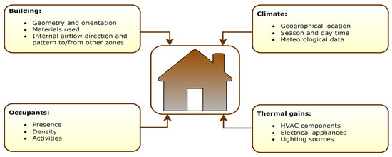
Figure 1.
Classification of factors affecting energy consumption in buildings.
Hence, the influence of these factors on building energy consumption has been a topic of focus. It is, therefore, logical to target the building sector when applying energy-saving techniques and rationalization measures.
By investing in energy efficiency, governments can achieve substantial energy cost savings across their facilities and demonstrate energy and environmental leadership. To improve the efficiency of existing and new facilities, governments need to incorporate energy efficiency policies and criteria into product procurement decisions. Using energy more efficiently can lower individual utility bills, reduce greenhouse gas emissions and other pollutants, create jobs, and meet growing energy demand.
1.1. Building Energy Demand in KSA
Typically, the weather in KSA is hot most of the year. Therefore, the need for air conditioning is logically high. According to the General Authority for Statistics, more than 99% of buildings in KSA are connected to the public electricity network (PEN). The energy consumed by buildings reached around 80% of the electricity produced in KSA [2], while air conditioning use accounts for 50% of that consumption [3]. The data related to energy consumption for various building sectors in KSA for the year 2021 has been collected from [4] and plotted in in Figure 2.
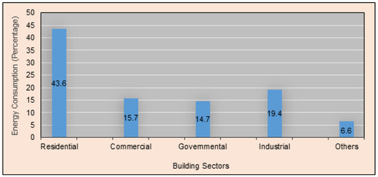
Figure 2.
Energy consumption for various building sectors in KSA [4].
The graph reflecting the number of equipment used for different energy demand types in KSA and the average operation hours per month for each is given in Figure 3 which has been plotted from statistical data collected from [2]. From this figure, it can be derived that air conditioning comes second after lighting. Figure 4 illustrates the breakdown of air conditioning equipment used in KSA [2]. Wall-mounted AC is the dominant equipment used for cooling in KSA. The bulk of these wall-mounted air conditioners are thermostat-based on/off actuated units, which makes them less effective and more energy-consuming.
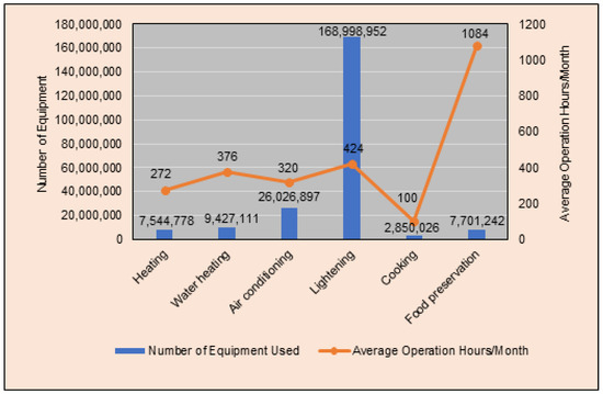
Figure 3.
The number of equipment used in KSA and their monthly average operation hours.
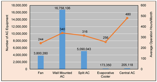
Figure 4.
AC equipment used in KSA and their monthly average operation hours.
Most buildings in the country are built with external walls, known as single-skin walls, made of concrete masonry units (CMU) with two holes. In the residential sector alone, more than 89.84% of dwellings are of this type [2]. Such walls are characterized by low thermal resistance [5]. The temperature inside such buildings without cooling is very high, especially in summer.
1.2. Energy Efficiency in KSA Buildings
Two-thirds of the buildings in KSA do not apply any type of thermal insulation [3], which is necessary to cut the overall consumption of cooling energy by preserving the anticipated atmosphere inside the edifice. Because average electricity bills are low, residents do not tend to reduce consumption, and consequently, a habit of buying low-efficiency devices is common. Additionally, there was a lack of product oversight and regulation to promote the use of energy-efficient appliances, and investment in energy efficiency was not encouraged for decades. However, lately, authorities have required that no building be connected to the PEN unless it has thermal insulation [3]. All these facts trigger the importance of identifying and taking some measures to rationalize the cooling energy demand in buildings. The next section highlights the issue.
1.3. Enhancing Energy Efficiency in Buildings
Table 1 classifies three groups of procedures and recommendations to moderate energy consumed for cooling in buildings. Procedures in the first group are related to the enhancement of the envelope’s thermal performance; the second group considers procedures concerning the cooling appliances used; the third group includes approaches related to the application of building automation.

Table 1.
Procedures and recommendations to reduce cooling energy.
1.4. Building Performance Simulation (BPS)
For a sustainable building sector, energy-efficient solutions should be adopted in one or more structure life-cycle-based on various BPS tools.
In this paper, a Simulink-based BPS model has been implemented as an extended study from a previous work [6]. The model considers the major heat and mass relocation processes that disturb the structure’s thermal performance in a real atmosphere. The objective of this BPS is to apply various rationalization measures and examine their impact on building thermal comfort and energy performance.
Three categories of rationalization measures have been identified, and one measure from each has been selected. Achieved results reflect the impact of applying these measures exclusively and mutually on building thermal comfort and energy consumption.
The manuscript is structured as follows. The literature review on related studies is presented in Section 2. The materials and methods used for the BPS model design are described in Section 3. The actual operation of the model and its response to selected rationalization measures are evaluated in Section 4. Finally, the conclusions and re-marks are provided in Section 5.
2. Literature Review
The process of designing an energy-efficient building is decision-based and comprises several tools. One such tool is BPS, which simulates buildings’ physical characteristics and performance, allowing designers to make sustainable design solutions. BPS can pinpoint places where energy use can be cut back, which could lead to long-term financial and environmental savings.
BPS concerns are addressed in [7]. The book—comprehensively accompanied by assessment, workouts, and investigation—covers all factors affecting the prediction and optimization of buildings’ energy use. A distinctive and inclusive overview of BPS for the whole structure life-cycle is delivered in [8]. The book begins with an introduction to the concepts of performance indicators and targets, followed by a discussion on the role of building simulation in performance-based building design and operation. Various building performance models have been studied in the literature. Two models of different scales were proposed and compared in [9]. It was shown that a second-order model is optimal. Tests on different types of building materials were presented in [10]. The study, carried out in Indonesia using Energy2D software, investigated the effect of these materials on the heat island intensity (HII). Another case study about the thicknesses of insulating materials was presented in [11]. The results clearly show this issue does not represent any desirable seasonal new furnish. A code was written in [12] to assess parameters manipulating the energy consumption in a residential building. A model for analyzing trials in the project stage of structure warming regulator systems was developed in [13]. The suggested method was verified using a Simulink model of a four-room building. Several reviews addressing building energy performance issues were conducted in [14,15,16]. The issues addressed included the practical approaches used, the input factors, the benefits gained, and the drawbacks. Paper [17] investigates how the spatial arrangement of thermal insulation and air gaps influences the overall thermal resistance of CMU wall systems. It proved that appropriate preparation of protection and air holes and accurate sizing could improve the overall thermal performance of CMU blocks. The economic and environmental impacts of energy efficiency programs associated with buildings for KSA have been evaluated in many studies in the literature. The existing status and prospects of BPS in the construction industry of KSA have been investigated in [18]. A survey has been carried out in this study with building industry professionals to investigate the existing practices regarding the use of BPS. Energy and environmental savings, achievable through the application of BPS, have been estimated by modeling a typical residential villa as a case study. Results of a study performed to propose potential energy-saving techniques for residential buildings in hot climates by critically examining existing and recent building types in KSA have been presented in [19]. In this paper, a model was designed using computer-based simulation software, DesignBuilder (DB), and the energy performance was then validated against the collected data. The study in [20] has focused on the effects of location and insulation material on the energy performance of a residential building by considering five climatic locations in KSA. Five commonly used insulation materials with different thermal characteristics were analyzed in this study under various climatic zones as per the Saudi Building Code 601/602. The findings indicate that the location significantly impacts the energy performance of the insulating materials.
3. Materials and Methods
3.1. Case Study Description
3.1.1. Location and Weather Characteristics
The considered laboratory is located on the first floor of a building situated at KKU in Abha, the administrative capital of the Aseer region South-West of KSA. Table 2 lists the location and weather data for Abha during the study period [21,22].
Table 2.
Location of Abha and its weather data during September 2022.
3.1.2. Building Characteristics
Figure 5a presents the envelope diagram of the modeled laboratory room, while Figure 5b illustrates the thermal processes within the room. The considered room is not surrounded by large objects that may cast shadows on it. The room’s physical features, the heat and mass components involved, the outside temperature variations, and the working hours of the laboratory room are the parameters governing the thermal behavior of the room and hence its energy consumption. These parameters are detailed in Table 3.
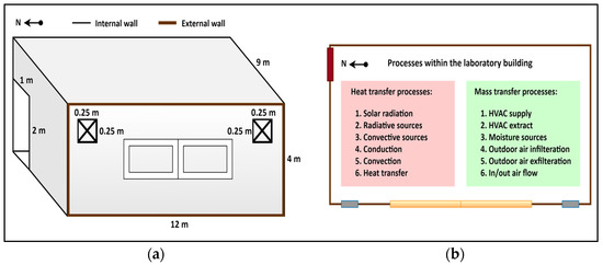
Figure 5.
The laboratory room. (a) Envelope diagram and (b) Thermal processes.
Table 3.
The parameters governing the thermal behavior of the laboratory room.
3.2. Case Study Simulation
The system simulation requires analysis of both heat and mass transfer processes, which define the thermal behavior of the laboratory room.
The variables that define the thermal behavior of the laboratory room are:
- The laboratory’s indoor temperature
- The laboratory’s thermal gains
- The laboratory’s thermal losses
- The energy accompanying heat sources inside the room.
The three modes of heat transfer are conduction, convection, and radiation. The mass transfer processes include the HVAC supply and extract, moisture sources, and outdoor air infiltration and exfiltration. Since this is a local simulation study, the recorded weather parameters have been adapted through spreadsheet manipulation on September 2022 data as a representative month that excludes extreme conditions. All essential parameters have been collected from the relevant national authorities and references [2,3,23]. The calculations used to prepare the data file for the simulation are based on the parameters listed in Table 3. The formulas used for linking these variables are explained in the following subsections.
3.2.1. Conduction Heat Transfer
The warm air loss in the laboratory room is due to conduction produced by the envelope and heat gain of occupants and apparatus. Conduction heat transfer through, into, and out of the room envelope is key in the building load and thermal response. To simplify the calculation, the conduction heat transfer rate through the wall is approximated to be 1D and described by:
- is the heat transfer rate (W);
- A is the area normal to the heat flow (m2);
- T1 and T2 are the surface temperatures at the wall sides;
- and R is the unit thermal resistance (m2K/W).
The room climate is effected by the heat movement within the room and given by:
where,
- is the input AC heat flow;
- is the measure of the coldness of the AC air;
- is the measure of the coldness of the room;
- is the rate of AC cool airflow;
- and is the specific heat of air.
3.2.2. Energy Balance at the External Surfaces
Energy balance at the external surfaces is given by [5]:
where,
- ew subscript is the considered external wall;
- is the rate at which incident solar radiation is absorbed by the external wall;
- is the rate of heat transfer from the envelope into the external wall;
- is the rate of convection heat transfer from external wall to the outdoor air;
- is the altercation of long wave radiation from other objects in the exterior environment (this term appears in a summation because the external wall will exchange radiation with a number of entities);
- and is the heat transfer from external wall to the surrounding soil.
The importance of exterior environmental conditions on this energy balance is obvious. It will be impacted by the position of the sun, conditions in the lower and upper atmosphere, the outdoor air temperature, wind velocity adjacent to the surface, soil temperatures, and the presence and temperature of atmospheric gases and clouds [5].
3.2.3. Internal Heat and Moisture Sources
Employing the uniform conditions assumption, the laboratory dry air mass balance equation can be expressed as:
- is the dry air infiltration through the room envelope;
- is the dry air transferred into the room;
- is the dry air delivered by the cooling system;
- and is the air movements leaving the room.
Similarly, the laboratory moisture mass balance equations can be expressed as:
The moisture-subscripted terms in Equation (5) are analogous to those air-subscripted terms used in Equation (4). The last term on the right denotes the variation of the contained mass of moisture.
Dry air and moisture flow rates are related by the humidity ratio (H in kgmoi/kgair) as:
Using Equation (4) in Equation (3) generates the joined dry air and moisture balances as:
Each internal surface shown in Figure 5 will experience convection, collect energy radiated from existing heat sources or cooling systems, and exchange long-wave radiation with other surfaces. Hence, the energy balance at the internal surface is given by:
where,
- subscript is the considered internal wall;
- is the incident solar radiation absorption rate;
- is the long wave radiation net exchange from other walls;
- is the received long wave radiation from heat sources;
- is the received long wave radiation from HVAC system;
- is the convective components of occupants and apparatus;
- and is the heat transfer into the envelope.
3.2.4. The Energy Associated with the Lighting, Occupants, and Apparatus
The heat loss caused by the CFLs used for lighting is determined using the same approach and equations as presented in [24]:
- is the lamps heat gain [kWh/yr];
- is the surface area [m2];
- is the amount of light falling onto a given surface area [lx];
- is the incandescent value [lm/W];
- is the hotness release factor;
- and is the yearly effective hours [h/yr].
The metabolic rate is the amount of energy used by an average person in a certain period. The unit for measuring this rate is met (1 met = 58.2 W/m2). Based on a formula explained in [25], the body surface area of the laboratory occupants is around 1.3 m2, and hence the calculated warmness formed by each occupant is 75.66 W [26].
The heat loss due to each laboratory apparatus is evaluated using Equation (9) with specifications obtained from respective data sheets [27,28,29,30,31,32,33]. Apparatus have been regarded as compact fluorescent lamps of comparable operating power. For estimating internal heat and moisture gains, nonresidential cooling and heating load calculations and data from [23] have been utilized.
3.2.5. The Amount of Heat Variation in the Room
This factor is determined by:
- is the outdoor temperature;
- is the corresponding thermal resistance of the room;
- and is the mass flow rate of air.
3.3. The Complete Model
Figure 6 illustrates the complete laboratory room Simulink thermal model. When running the model, it loads the required information, which defines the thermal behavior from a data file. The outdoor temperature readings collected during the laboratory sessions were used as a changing input to the model through a spreadsheet block. When the AC is on, it blows cold air at a predefined set (TAC) and a fixed flow rate. A regulator included in the subsystem allows selected degree variations around TAC. The Communication Laboratory Building subsystem computes the building temperature differences. It compares the thermal gain from the AC and the building thermal losses to determine the actual indoor temperature. The desired set point is subtracted from the comparison result to check if there is an error signal (temperature difference). The consumed energy and its cost are computed by the calculator subsystem.
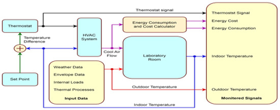
Figure 6.
The laboratory room Simulink thermal model.
4. Results and Discussions
This section presents and discusses the model simulation results. The outdoor temperature readings were recorded during the actual laboratory sessions in September 2022. The starting temperature set point was set to 20 °C as this is a common behavioral practice noticed within the university community. The initial indoor temperature was assumed to be 26 °C.
4.1. Actual Case Results
The actual case results are given in Figure 7 and Figure 8. The regulator signal produced from the thermostat to adjust the AC operation in the actual case is illustrated in Figure 7. Figure 8 presents the indoor–outdoor temperatures for the same case. The indoor temperature graph clearly reveals the oscillations around the set point.
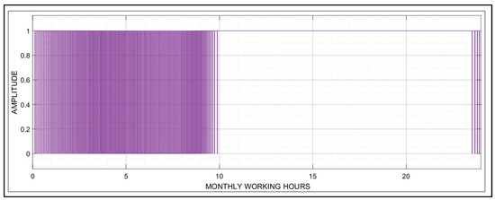
Figure 7.
The thermostat signal (actual case).
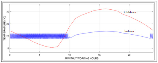
Figure 8.
The indoor–outdoor temperature (actual case).
4.2. Rationalized Case Results
Three selected recommendations from the list categorized in Table 1 for energy rationalization have been applied individually to the laboratory building model to check the effect of each on the building’s thermal behavior.
When the desired temperature set point is changed to the range recommended by ASHRAE, which is 23 °C, the task of the cooling system needed to catch the anticipated degree varied extensively following the thermostat signal, as shown in Figure 9. The indoor–outdoor temperature graph for this case is given in Figure 10.
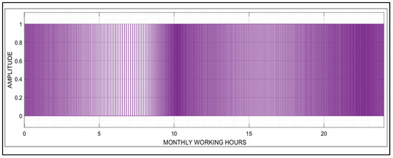
Figure 9.
The thermostat signal (23 °C set point case).
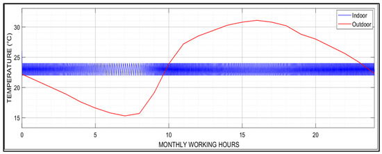
Figure 10.
The indoor–outdoor temperature (23 °C set point case).
To see the effect of changing the materials used in constructing the building, a CMU with enhanced thermal conductivity proposed in [17] has been assumed for the building walls. This enhancement increases the equivalent thermal resistance for the whole building by more than 66%, considering all other envelope materials remain unchanged. The control signal and the indoor–outdoor temperature when this building envelope-related measure is applied are illustrated in Figure 11 and Figure 12, respectively.
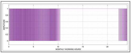
Figure 11.
The thermostat signal (enhanced CMU case).
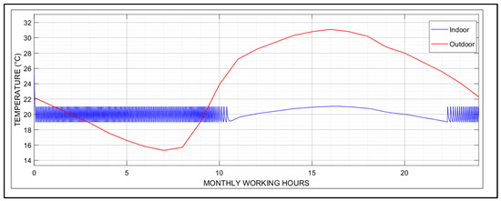
Figure 12.
The indoor–outdoor temperature (enhanced CMU case).
AC systems can use thermostats with a built-in PID controller to accomplish smoother operation by gaining the capability to regulate their output. This approach has been followed to detect the effect of improving the AC system behavior. The control signal and indoor temperature results after applying this measure are presented in Figure 13 and Figure 14.
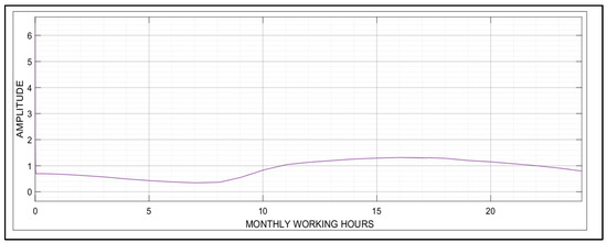
Figure 13.
The thermostat signal (PID controller case).
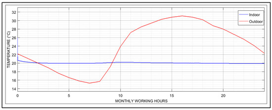
Figure 14.
The indoor–outdoor temperature (PID controller case).
All selected rationalization measures were applied simultaneously to examine their collective effect on the case model. The result graphs for the control signal and the indoor–outdoor temperature for this case are shown in Figure 15 and Figure 16, respectively.
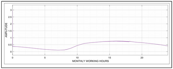
Figure 15.
The thermostat signal (collectively rationalized case).
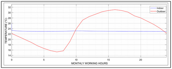
Figure 16.
The indoor–outdoor temperature (collectively rationalized case).
4.3. Energy Consumption and Cost Results
Figure 17 illustrates the energy consumed to cool the building for each case. The monthly energy cost for each case is presented in Figure 18. It should be noted that the use of the PID controller, despite smoothing the operation of the AC, increases the energy consumed and hence, the cost compared to the actual case. This increase can be justified by the continuous operation status of the AC with a PID-controlled thermostat compared to the fluctuating operation of the AC with a relay-controlled thermostat.
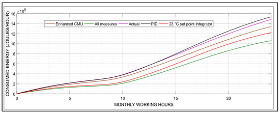
Figure 17.
The monthly cooling energy demand for each case.
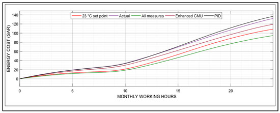
Figure 18.
The monthly cooling energy cost for each case.
Finally, Figure 19 illustrates the consumed energy, the monthly cost, and the rationalization percentage for each measure considered in this study compared to the actual case.
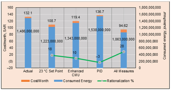
Figure 19.
The monthly performance assessed for each case.
5. Conclusions and Remarks
In this study, a zonal modeling approach is applied to judge the influence of the location and the construction materials used on the indoor temperatures in a university building in KSA. The study was carried out in September 2022, during which heavy use of air-cooling activities took place all over the country. The cost of energy consumed for cooling the building to a desired indoor temperature was also calculated. Three categories of measures to rationalize building cooling energy consumption were presented and discussed. Three selected measures were applied to associate the building performance before and after rationalization. Each measure was first applied individually, and then all three measures were used collectively. The best energy rationalization performance reached for an individual action was 17.72%, and it was accomplished when we raised the set point of room temperature from 20 °C to 23 °C. However, a total reduction of 28.38% in energy consumption and cost was obtained when all three selected measures were applied collectively. The results obtained draw attention to various points. Firstly, energy can be significantly saved by raising space cooling temperatures while maintaining standard thermal comfort, which indicates that occupant behavior can form part of a cost-effective solution to support the transformation of energy systems. Secondly, constructing buildings with high thermal insulation characteristics is more beneficial from an economic and environmental perspective. This can be achieved by building walls using new low thermal conductivity CMUs. Finally, using energy-efficient HVAC systems can save energy and money and reduce global warming and climate change. Reducing energy demand and applying rationalization measures is a huge challenge that requires coordinated actions across policy, regulation, building codes, standards, facilities management, and more research and development. It is worth mentioning that the processes for forming prototypical assembly and procedure design used here are functional to other cases or future work aimed at the same topic.
Funding
This research was funded by King Khalid University, grant number RGP2/400/44.
Data Availability Statement
No new data were created or analyzed in this study. Data sharing is not applicable to this article.
Acknowledgments
The author extends his appreciation to the Deanship of Scientific Research at King Khalid University for funding this work through large Group Research Project under grant number RGP2/400/44.
Conflicts of Interest
The author declares no conflict of interest.
References
- Kaynakli, O. Thermal insulation: A review of the economical and optimum thermal insulation thickness for building applications. Renew. Sustain. Energy Rev. J. 2012, 16, 415–425. [Google Scholar] [CrossRef]
- General Authority for Statistics Electricity Energy Statistics. 2019. Available online: https://www.stats.gov.sa/sites/default/files/hst_ltq_lkhrbyy_-_rby_0.pdf (accessed on 10 September 2022).
- Saudi Energy Efficiency Center Annual Report. 2021. Available online: https://www.seec.gov.sa/sites/default/files/blog_files/annual-report-2018.pdf (accessed on 12 September 2022).
- Saudi Central Bank Economic Reports. Available online: https://www.sama.gov.sa/en-US/EconomicReports/Pages/report.aspx?cid=126 (accessed on 25 August 2022).
- Al-Jabri, K.; Hago, A.W.; Al-Nuaimi, A.; Al-Saidy, A. Concrete blocks for thermal insulation in hot climate. Cem. Concr. Res. 2005, 35, 1472–1479. [Google Scholar] [CrossRef]
- Suliman, F.E.M.; Elsheikh, E.A. Thermal modeling and simulation of a laboratory building for cooling energy consumption. J. Eng. Res. 2021, 9, 174–190. [Google Scholar] [CrossRef]
- Beausoleil-Morrison, I. Fundamentals of Building Performance Simulation; Routledge, Taylor & Francis: New York, NY, USA, 2020; ISBN 9781003055273. [Google Scholar]
- Hensen, J.L.M.; Lamberts, R. Building Performance Simulation for Design and Operation; Spon Press: New York, NY, USA, 2011. [Google Scholar]
- Yashen, L. Modeling the Thermal Dynamics of a Single Room in Commercial Buildings and Fault Detection. Master’s Thesis, The University of Florida, Gainesville, FL, USA, 2012. [Google Scholar]
- Wonorahardjo, S.; Sutjahja, I.S.; Mardiyati, Y.; Andoni, H.; Thomas, D.; Achsani, R.A.; Steven, S. Characterizing Thermal Behavior of Buildings and Its Effect on Urban Heat Island in Tropical Areas. Int. J. Energy Environ. Eng. 2019, 11, 129–142. [Google Scholar] [CrossRef]
- Carlinia, M.; Zillib, D.; Allegrinia, E. Simulating Building Thermal Behavior: The Case Study of The School of The State Forestry Corp. Energy Procedia 2015, 81, 55–63. [Google Scholar] [CrossRef]
- Sjösten, A.; Olofsson, T.; Golriz, M. Heating Energy Use Simulation for Residential Buildings. In Proceedings of the Eighth International IBPSA Conference, Eindhoven, The Netherlands, 11–14 August 2003; pp. 1221–1226. [Google Scholar]
- Lapusan, C.; Balan, R.; Hancu, O.; Plesa, A. Development of a Multi-Room Building Thermodynamic Model Using Simscape Library. Energy Procedia 2016, 85, 320–328. [Google Scholar] [CrossRef]
- Krstić, H.; Teni, M. Review of Methods for Buildings Energy Performance Modelling. IOP Conf. Ser. Mater. Sci. Eng. 2017, 245, 042049. [Google Scholar] [CrossRef]
- Amara, F.; Agbossou, K.; Cardenas, A.; Dubé, Y.; Kelouwani, S. Comparison and Simulation of Building Thermal Models for Effective Energy Management. Smart Grid Renew. Energy 2015, 6, 95–112. [Google Scholar] [CrossRef]
- Foucquier, A.; Robert, S.; Suard, F.; Stephan, L.; Jay, A. State of The Art in Building Modeling and Energy Performances Prediction: A Review. Renew. Sustain. Energy Rev. J. 2013, 23, 272–288. [Google Scholar] [CrossRef]
- Mooneghi, M.A.; Kargarmoakhar, R.; Chowdhury, A.G. Improving the Thermal Performance of Concrete Masonry Blocks. Fla. Civ. Eng. J. 2015, 1–10. Available online: https://www.academia.edu/24445141/Improving_the_Thermal_Performance_of_Concrete_Masonry_Blocks (accessed on 15 September 2022).
- Ahmed, W.; Asif, M.; Alrashed, F. Application of Building Performance Simulation to Design Energy-Efficient Homes: Case Study from Saudi Arabia. Sustainability 2019, 11, 6048. [Google Scholar] [CrossRef]
- Alyami, M.; Omer, S. Building energy performance simulation: A case study of modeling an existing residential building in Saudi Arabia. Environ. Res. Infrastruct. Sustain. 2021, 1, 035001. [Google Scholar] [CrossRef]
- Alyami, S.H.; Alqahtany, A.; Ashraf, N.; Osman, A.; Aldossary, N.A.; Almutlaqa, A.; Al-Maziad, F.; Alshammari, M.S.; Al-Gehlani, W.A.G. Impact of Location and Insulation Material on Energy Performance of Residential Buildings as per Saudi Building Code (SBC) 601/602 in Saudi Arabia. Materials 2022, 15, 9079. [Google Scholar] [CrossRef] [PubMed]
- Long-Term Weather Forecast Abha, Saudi Arabia. Available online: https://www.weather-atlas.com/en/saudi-arabia/abha-long-term-weather-forecast (accessed on 15 September 2022).
- Global Solar Atlas Abha, Saudi Arabia. Available online: https://globalsolaratlas.info/map?c=18.216633,42.504044,11&s=18.216428,42.50436&m=site (accessed on 15 September 2022).
- ASHRAE. 2017 ASHRAE Handbook of Fundamentals; Technical Report; American Society for Heating, Refrigeration, and Air-Conditioning Engineers: Atlanta, GA, USA, 2017. [Google Scholar]
- Zell, E.; Gasim, S.; Wilcox, S.; Katamoura, S.; Stoffel, T.; Shibli, H.; Engel-Cox, J.; Al Subie, M. Assessment of Solar Radiation Resources in Saudi Arabia. Solar Energy 2015, 119, 422–438. [Google Scholar] [CrossRef]
- Suszanowicz, D. Internal Heat Gain from Different Light Sources in the Building Lighting Systems. In E3S Web of Conferences, Proceedings of International Conference on Energy, Environment and Material Systems (EEMS2017), Polanica-Zdroj, Poland, 13–15 September 2017; EDP Sciences: Courceboeufs, France, 2017. [Google Scholar] [CrossRef]
- Body Surface Area. Available online: http://www-users.med.cornell.edu/~spon/picu/calc/bsacalc.htm (accessed on 20 August 2019).
- ANSI/ASHRAE 55-2017; Thermal Environmental Conditions for Human Occupancy, ASHRAE Standard. American Society for Heating, Refrigeration, and Air-Conditioning Engineers: Atlanta, GA, USA, 2017.
- LISIN High-Pressure Exhaust Fan Model DVN-101/DVN-121 Catalogue. Available online: http://ridonelectrical.com/index.php?route=product/product&path=66&product_id=58 (accessed on 15 August 2019).
- Residential Split Systems From 0.6 to 5 T. R. Available online: http://www.aireclima.com/TRANE/pdfs/yellow/yellow.pdf (accessed on 15 September 2019).
- Philips Fluorescent Lamp Data Sheet. Available online: https://www.lighting.philips.com/main/prof (accessed on 20 October 2019).
- Com3lab: The Compact Electronics Laboratory. Available online: http://www.hanmacco.com/images/_contents/file003/P1.pdf (accessed on 15 September 2019).
- DELL OPTIPLEX 790 Technical Guide. Available online: https://i.dell.com/sites/doccontent/shared-content/data-sheets/en/Documents/optiplex-790-tech-guide.pdf (accessed on 30 August 2019).
- DELL INSPIRON N5110 Setup Guide. Available online: https://downloads.dell.com/manuals/all-products/esuprt_laptop/esuprt_inspiron_laptop/inspiron-15r-n5110_setup%20guide_en-us.pdf (accessed on 30 August 2019).


Disclaimer/Publisher’s Note: The statements, opinions and data contained in all publications are solely those of the individual author(s) and contributor(s) and not of MDPI and/or the editor(s). MDPI and/or the editor(s) disclaim responsibility for any injury to people or property resulting from any ideas, methods, instructions or products referred to in the content. |
© 2023 by the author. Licensee MDPI, Basel, Switzerland. This article is an open access article distributed under the terms and conditions of the Creative Commons Attribution (CC BY) license (https://creativecommons.org/licenses/by/4.0/).