Abstract
One of the primary challenges in cable-stayed bridges is to assess the service performance of stay cables in response to applied loads and ensure that they meet safety requirements. This paper proposes a new strategy to analyze the time-varying reliability of the ultimate load-carrying capacity of stay cables under resistance and stress uncertainty conditions. Initially, we employ the frequency-squeezing processing (FSP) technique within the vibration frequency method (VFM) to enhance the accuracy and effectiveness of cable force identification through field measurement. Subsequently, we thoroughly discuss and establish the statistical characteristics and probabilistic models of stress, including both slow-varying trend and fast-varying trend components, as well as resistance considering the strengthening deterioration effect. The slow-varying trends of the cable forces are extracted using the moving average method (MAM), and both the extracted slow variation and the fast-varying trend components are analyzed in detail. Finally, we introduce a Gaussian process-based surrogate model to assess the time-varying structural reliability by analyzing the associated limit-state function for the ultimate load capacity of the stay cables. In this study, the proposed strategy is applied to quantify the ultimate load-carrying reliability of a stay cable under the uncertainty of the coupled action of corrosion and fatigue. Compared with conventional reliability analysis, the failure probability interval estimation shows the uncertainty boundaries and provides specific years of reliability failure, which can serve as an important reference for bridge maintenance and strengthening.
1. Introduction
Existing bridge-like structures, such as cable-stayed and multi-span bridges, involve complex interactions between materials and design elements. Recent studies have aimed to address various aspects of this response. Yang et al. [1] investigated the mechanical properties of displacement-amplified mild steel bar joint dampers, providing insights into the behavior of mild steel bars under load. Luo et al. [2] explored damage mechanisms in rib-to-deck welded joints through numerical simulations, enhancing our understanding of potential failure points. Furthermore, Luo et al. [3] examined the bond performance of helically ribbed GFRP bars embedded in ultra-high-performance concrete (UHPC), highlighting critical factors affecting bond strength. In addition to these studies, the integrity of stay cables is crucial for maintaining the structural safety and stability of cable-stayed bridges [4,5,6]. As the key components, the stay cables are susceptible to various forms of damage, including stress, fatigue, and corrosion, which can compromise their service performance and endanger bridge users. To reduce the likelihood of stay cable failures, it is imperative to conduct a time-varying reliability assessment. By monitoring the condition and response of cables to various loads or stresses, engineers can promptly identify potential issues and take corrective action.
In recent decades, several methodologies for time-varying reliability assessment have been proposed for the condition assessment of stay cables in existing cable-stayed bridges, including visual inspection-based approaches and structural health monitoring (SHM)-based methods [7,8,9,10]. Visual inspections, along with non-destructive evaluation techniques like electromagnetic and ultrasonic inspections, can aid in monitoring cable conditions and detecting potential issues such as broken wires, which are crucial for assessing structural reliability [11]. Additionally, time-varying cable tension identification methods, like the adaptive approach based on improved variational mode decomposition, can provide accurate insights into cable conditions over time, contributing to reliability assessment [12]. Integrating BIM technology for time-varying structural safety analysis can further improve reliability assessments by considering component-level evaluations and system safety impacts, especially in scenarios like long-term corrosion analysis of underground pipelines and short-term seismic load analysis of building structures [7]. On the other hand, the rapid development of sensing techniques has led to the emergence of structural health monitoring (SHM) systems, characterized by their ability to acquire structural responses, extract features, and assess structural conditions. Time-varying reliability assessment of stay cables in SHM is crucial for ensuring the safety and performance of bridges [13]. Techniques like time–frequency reassignment algorithms can efficiently identify time-varying cable tension, aiding in the real-time condition monitoring of bridges [14]. Incorporating stochastic structural dynamics with SHM data and random loadings can enhance reliability assessment, considering factors like atmospheric turbulence and sensor outputs [15]. Monitoring internal forces during the construction stages of bridges is essential, with methods like punctiform time-varying reliability calculations providing insights into stress states and aiding in safety evaluations [16]. Overall, integrating time-varying reliability assessment with SHM techniques offers a comprehensive approach to ensuring the structural integrity and safety of stay cables in bridges.
As a precondition for a valid assessment of time-varying reliability, recent studies have made significant advancements in the identification of cable forces in stay cables [17,18]. The vibration frequency-based method (VFM) is commonly utilized due to its simplicity, speed, and cost-effectiveness. VFMs enhance the accuracy of determining cable forces in cable-stayed bridges by considering various factors often overlooked in traditional methods. These techniques address issues like boundary conditions, bending stiffness, and support constraint stiffness, leading to more precise estimations [19]. Additionally, the use of thin rod vibration sensors with high-sensitivity Fiber Bragg grating (FBG) technology allows for accurate cable force measurements, even in challenging scenarios like measuring forces in steel strand-type bracing cables [20]. Automation of vibration-based tension estimation through stochastic subspace identification (SSI) methods further improves accuracy by continuously identifying stable modal frequencies and efficiently computing cable tensions in real time [21]. By integrating these advancements, cable force identification in cable-stayed bridges becomes more reliable and effective, ensuring the structural integrity and long-term serviceability of the bridges.
Timely online identification of time-varying cable forces was more relevant for reliability spectrum assessment in engineering practice than offline processing. Over the past decade, the literature on time-varying reliability analysis has explored another approach aimed at saving significant computational budgets while retaining the benefits of simulation methods: surrogate model-assisted methods. Surrogate models, which are inexpensive approximations of the original computational model, have consistently demonstrated superior performance when combined with traditional simulation methods. Initially, simple polynomial response surface models (RSMs) were built from a set of well-designed computer experiments, and these RSMs were then used instead of the original computational model to approximate the solution equation. Drawing on experience from the field of machine learning, this process has evolved into a more sophisticated approach known as active learning. In active learning, surrogate models are not merely proxies for the original computational model but are tools to help efficiently explore the space of random input variables. Active learning techniques have gained traction in structural reliability analysis due to their ability to efficiently solve complex problems with reasonable computational resources [22,23]. These methods, aimed at enhancing the efficiency and accuracy of reliability analysis in engineering practice, often leverage surrogate models and sophisticated reliability estimation algorithms. For instance, Peijuan introduced a novel active learning method based on the learning function U, which significantly improved the convergence speed of the AK-MCS method for problems with a connected domain of failure [24]. Considering the importance of time-varying reliability in assessing the structural integrity of bridge-like structures, it is essential to explore advanced methods and control strategies. She et al. [25] introduced an improved wolf pack algorithm for structural reliability analysis, offering a robust approach for evaluating the reliability of various structural elements over time. This method enhances the ability to predict and mitigate potential failures in dynamic environments. Additionally, Zhang [26] investigated the application of tuned mass dampers (TMDs) for flutter vibration control in long-span bridges. The active rotary inertia driver system presented in this study provides promising solutions for controlling vibrations and improving the stability of bridge structures. Integrating these approaches can significantly enhance the time-varying reliability assessments and overall performance of bridge-like structures. Additionally, Ehre demonstrated the effectiveness of combining dimensionality reduction and surrogate modeling to analyze high-dimensional, computationally expensive engineering models [27]. By employing an active learning procedure, they achieved improved error control. These studies collectively underscore the potential of active learning in reliability analysis, particularly in enhancing efficiency and accuracy.
The use of surrogate modeling and reliability estimation algorithms in the structural health monitoring of cable-stayed bridges offers significant advantages in terms of computational efficiency and predictive capability. However, these methods are not without limitations and uncertainties that can impact the accuracy and reliability of the assessments. Surrogate models, while effective in reducing computational costs, may introduce errors due to model simplifications and assumptions. Additionally, the reliability estimation algorithms employed are subject to variability stemming from input data quality and methodological choices. Addressing these potential sources of error and variability is crucial for enhancing the credibility of reliability assessments conducted using these methods [28,29,30].
2. Methodology
2.1. Generalized Framework
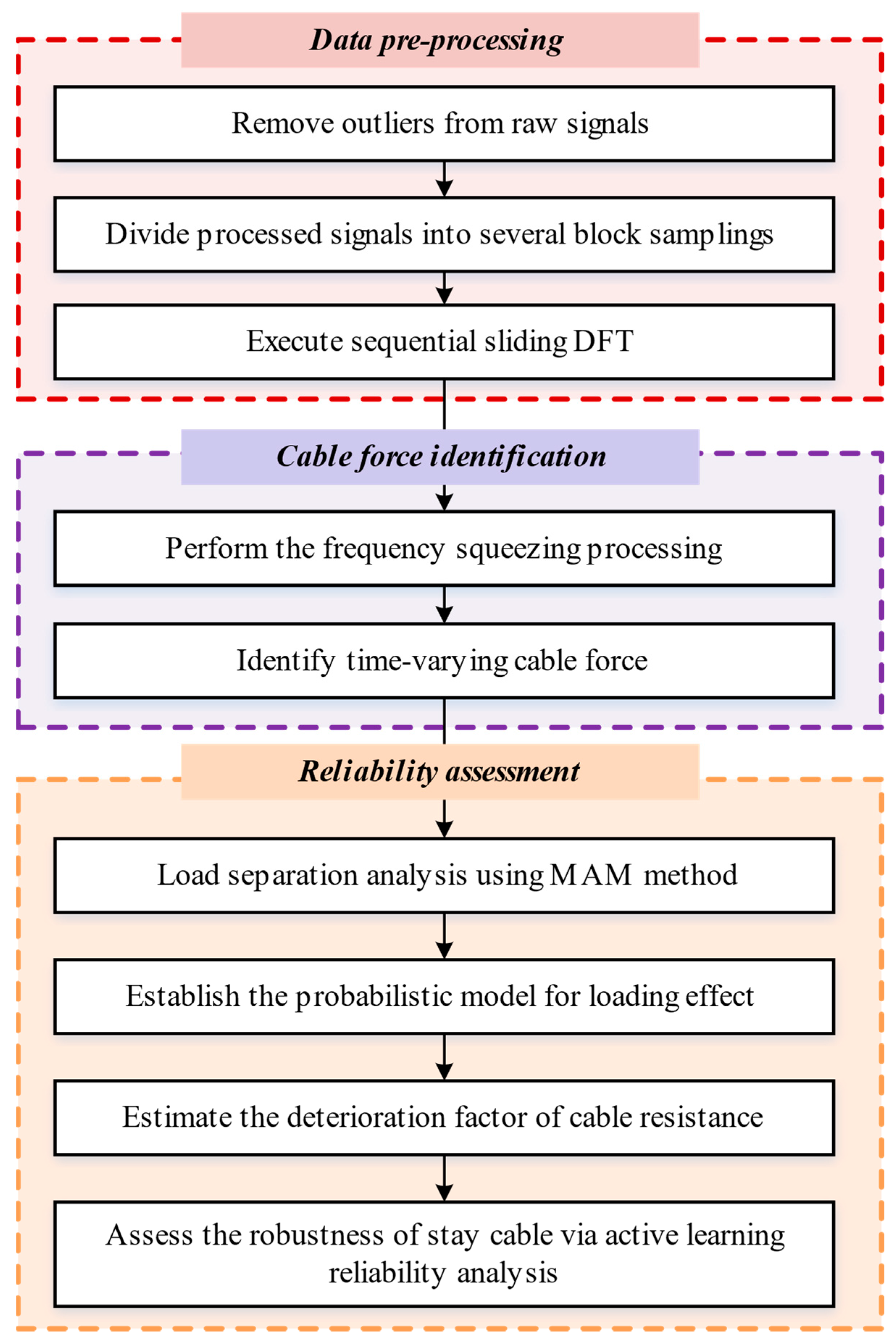
As depicted in Figure 1, the proposed framework for analyzing the time-varying reliability of parallel wire cables includes three main steps: data pre-processing, cable force identification, and reliability assessment. The initial phase of the procedure includes the removal of outliers, such as the elimination of significant errors, and the application of low-pass filtering to the obtained vibration signals. Following this, long-processed signals can be segmented into adjustable block samplings based on factors such as the target fundamental frequency of parallel wire cables. Subsequently, the sequential sliding discrete Fourier transform (DFT) is performed to obtain the raw frequency spectrum. In the second phase, we utilize an algorithm named frequency-squeezing processing (FSP) to enhance the clarity of the raw frequency spectrum in the vibration frequency method (VFM). This approach aids in identifying the time-varying force of parallel wire cables through the proposed frequency spectrum. Additionally, we can employ active learning reliability analysis to evaluate safety by estimating the probability distribution of the resistance capacity and load effect for the parallel wire cables.
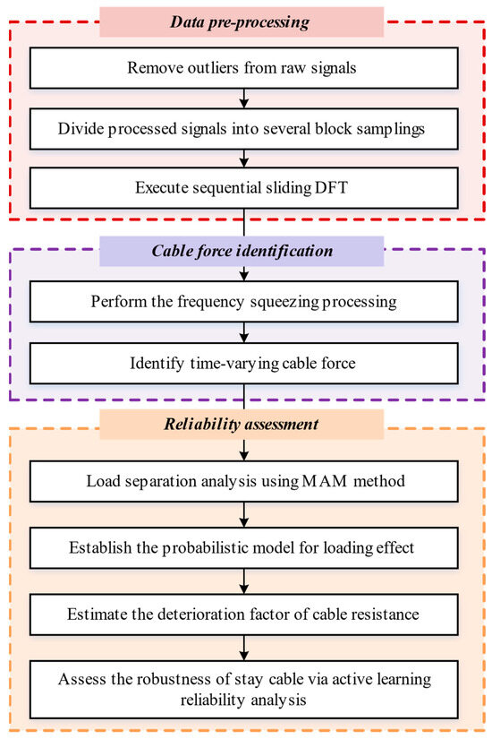
Figure 1.
Schematic diagram of FSP-VFM-based active learning for reliability analysis of parallel wire cables.
2.2. Cable Force Identification Using FSP-VFM
2.2.1. Vibration Frequency-Based Method
In the context of cable-stayed bridges, stay cables are consistently subjected to a high-stress, micro-vibration environment during operation. The vibration frequency method (VFM) stands as the prevailing and cost-effective modality for identifying cable forces. Influenced by bending stiffness, support conditions, and concentrated mass, VFM involves the derivation of the cable vibration equation and the establishment of the mapping relationship between the cable tension and the natural frequency. It is imperative to acknowledge the presence of several assumptions inherent in the analysis of the vibration equations, including the uniform distribution of cable mass with equal cross-section and material elasticity, and the exclusion of rotational inertial mass, shear deformation, and the sag effect [21]. Hence, by incorporating considerations of bending rigidity, end support conditions, and centralized mass in the span, a unified equation is formulated to delineate the relationship between the cable force and the fundamental frequency of the cable:
where denote the influencing factors attributed to support conditions, concentrated mass, and bending stiffness, respectively; represents the fundamental frequency; denotes the mass per unit length; denotes the centralized mass in the middle of the span; is the free length of the cable; and is the bending rigidity of the cable. When the length-to-diameter (L/D) ratio is less than or equal to 150, and only the mass and tension force terms are taken into account, the mapping relationship between cable force and natural frequency can be simplified and determined:
where denotes the natural frequency of the mode and denotes the e-th identified mode.
2.2.2. Frequency-Squeezing Processing
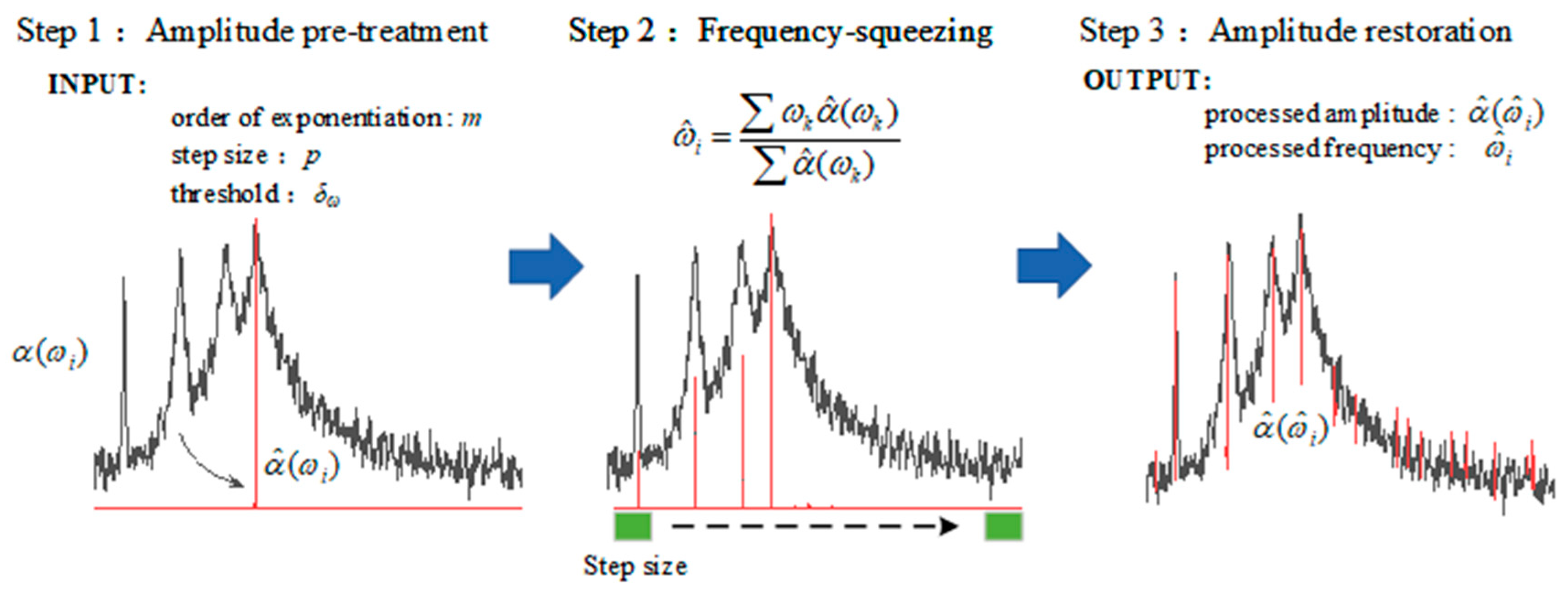
The utilization of the extracted frequency under FSP can significantly enhance the accuracy of identifying cable force, particularly in the presence of complex noises and measurement errors. A schematic diagram of FSP, depicted in Figure 2, encompasses three primary steps, which will be detailed in the following section [31,32].

Figure 2.
A schematic diagram of FSP.
The initial stage of the amplitude pretreatment for the raw frequency spectrum involves the normalization of the spectrum amplitude within the range of 0 to 1. Subsequently, the amplitude undergoes a “shaping” process by raising it to the power of for further computational treatment. The amplitude pretreatment process can be formally described as follows:
where and are the spectral amplitudes before and after processing, respectively; is the sampling frequency point from a vector ; and can be set as integer multiples of 10 to reduce rapidly the amplitude of the peak nearby.
Step 2: Frequency squeezing is utilized for the pre-processing of the signal. The frequency is substituted with the centroid coordinate of a graph, which is formed by the spectral lines by taking the 2p + 1 (p ≥ 1) spectral lines into account.
where p and K are the user-specified steps and the signal length, respectively. Then, the step is executed until the convergence criterion is met. The convergence criterion is defined as follows.
where s is the number of iterations and denotes the threshold.
In the third step of the process, the focus is on restoring the amplitude and adjusting the zero settings. As the amplitude magnitude has been normalized in the initial step, our objective is to preserve accurate amplitude information. Subsequently, the original amplitude vector is aligned with the newly generated frequency vector based on their respective order of subscripts. Furthermore, the amplitude between the edges and the cluster of aggregated frequency points is then adjusted to zero, which can be written as follows:
where Ω is the set of frequency subscripts corresponding to the set of zero amplitude. is the indicator to determine the abnormal frequency, which is suggested to be set as 0.01 or 0.001 times .
In scenarios with a low signal-to-noise ratio, the presence of multiple candidate peaks due to noise can heighten uncertainty in peak selection. FSP adjusts the shape of the local spectrum (derived from the discrete Fourier transform of the cable’s time history) to align with its nearby natural frequency without altering its magnitude, thereby enhancing the accuracy of frequency identification. A significant advantage of employing FSP in structural health monitoring is the elimination of the laborious manual peak-searching process. Instead, FSP automatically provides the expected value of the fundamental frequency in the relationship between cable force mapping and frequency. This enables automatic, real-time, and precise cable force identification, laying the groundwork for subsequent time-varying reliability assessment.
2.3. Resistance Deterioration Model of Parallel Wire Cables
2.3.1. Daniel’s Model for the Strength of a Parallel Wire Cable
As depicted in Figure 3, the strength of a bundle of parallel wires can be evaluated through the application of a parallel system model (mechanical model) [33]. In cases where the number of components in the system () exceeds 150, the strength of the parallel system demonstrates a normal distribution with a mean value
and standard deviation
where and can be inferred from
where is the probability density function (PDF) of the parallel wire strength and is the solution of
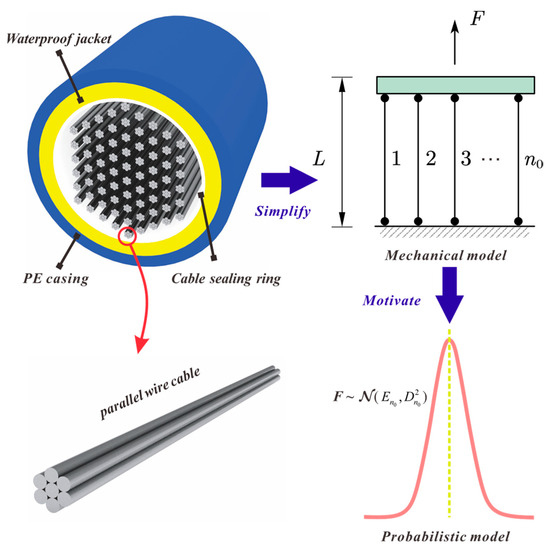
Figure 3.
Parallel wire cables.
And is the cumulative distribution function (CDF) of the Weibull distribution that is described as
where and denotes the shape and scale parameters, respectively; represents the proportionality parameter of the Weibull distribution and can be deduced from
where denotes the autocorrelation function of the wire’s ultimate load capacity; denotes the associated length of the wire; is the sample length of wire in the test of the wire’s ultimate load capacity; and denotes the correction factor of . In general, the quality of the wire in a new cable is more homogeneous, resulting in a larger and a correspondingly smaller . As the cable ages, corrosion gradually infiltrates the internal structure, leading to varying degrees of corrosion along the cable’s length. Consequently, the diminishing will cause an increase in the . In conclusion, these two correlation parameters have a significant effect on the ultimate load-carrying capacity of the parallel wire cable, and the selection of still adheres to empirical guidelines.
2.3.2. Strength Deterioration Factor under Coupled Corrosion–Fatigue Influence
The deterioration of cable resistance in cable-stayed bridges is a common concern, as factors such as corrosion and fatigue can lead to degradation. Furthermore, high stress can make cables more susceptible to corrosion, resulting in rust and eventual breakage [34,35]. This degradation can take various forms, including stress corrosion cracking, pitting corrosion, corrosion fatigue, and hydrogen embrittlement, all of which weaken the wire and shorten the cable’s lifespan. The theory of fatigue damage accumulation posits that the failure times of undamaged wires within the average stress range are assumed to be independent and identically distributed (i.i.d). The wire with the shortest failure time is the first to break, leading to a redistribution of stresses in the remaining wires. The theory also generalizes the Weibull distribution that gives the initial failure time for the number of failure cycles of the wire in the stress range
where , and are the parameters corresponding to experimental test estimates; is a parameter related to the cross-sectional area of the cable. Faber et al. investigated the mechanisms of fatigue stress degradation utilizing ultrasonic inspection. They proposed functional models for the resistance degradation of main cables and hanger cables under coupled corrosion–fatigue conditions. Drawing from the findings of Faber et al. [33], interpolation of the strength deterioration factor of coupled corrosion–fatigue steel wires was performed for 20 years:
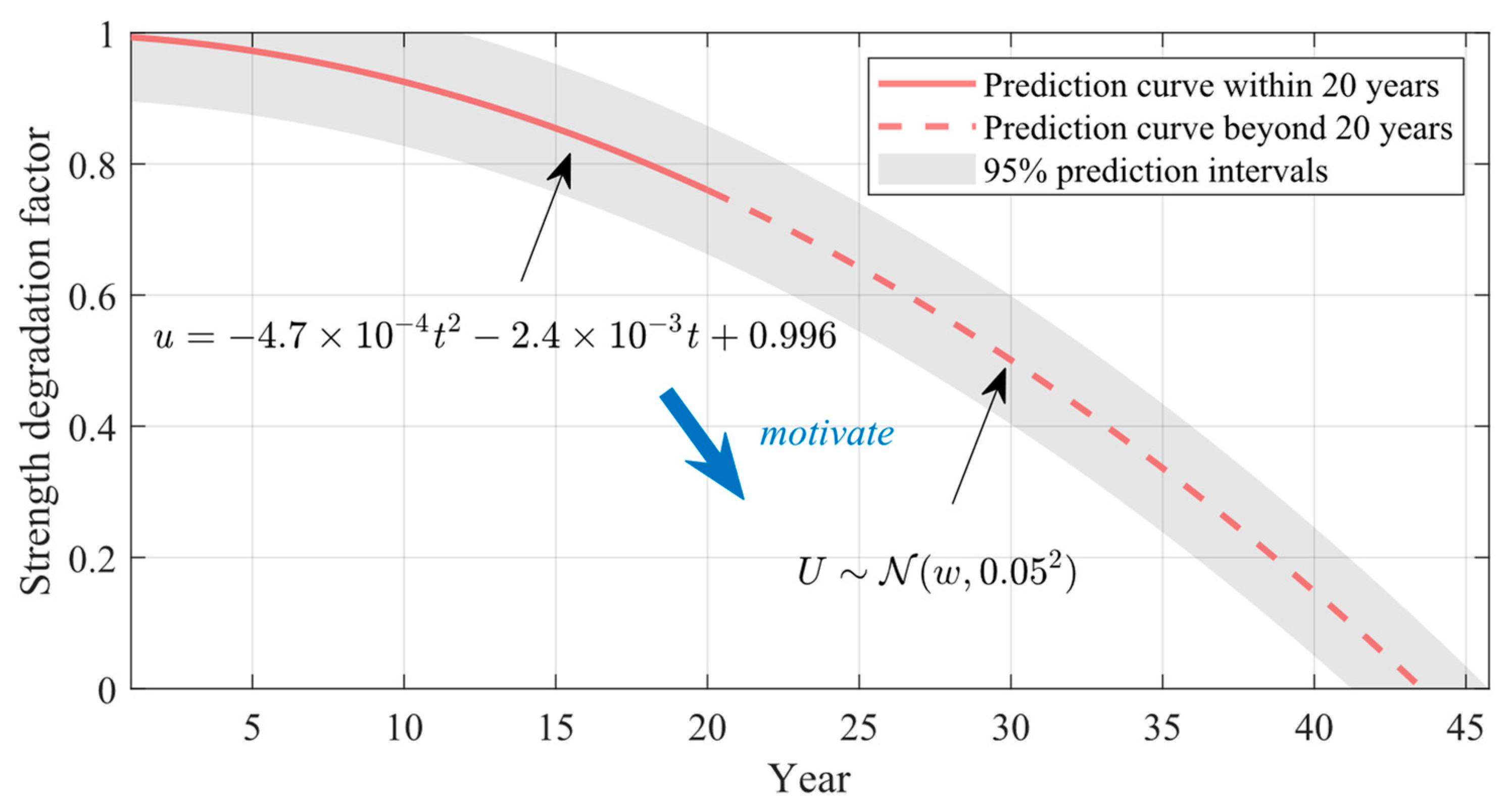
where and denote the strength degradation factor and service year, respectively. As shown in Figure 4, the red line indicates the strength deterioration factor of the prediction curve under coupled corrosion–fatigue influence within 20 years. The nonlinear nature of the fatigue corrosion effect curve significantly contributes to the rapid decrease in cable strength. And the meticulous determination of the strength degradation factor is imperative in evaluating the reliability of parallel wire cables. Hence, to identify the strength degradation factor with coupled corrosion fatigue beyond 20 years, we introduce a probabilistic model using a Gaussian distribution with a 5% coefficient of variation:
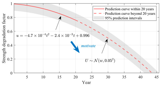
Figure 4.
A probabilistic model for strength degradation factor under coupled corrosion–fatigue effect.
The red dashed line represents the expectation of strength deterioration factor under coupled corrosion–fatigue influence beyond 20 years, based on the extrapolation of the case within 20 years. Meanwhile, considering the uncertainty of the prediction curve beyond 20 years, the grey area represents the 95% confidence interval (confidence level , ) in the Gaussian distribution.
2.4. Active Learning Reliability Analysis Based on GP Modeling
The basis of reliable active learning revolves around minimizing the computational cost of simulation algorithms. This is achieved by employing a surrogate model that serves as a cost-effective approximation of the limit-state function, which could be prohibitively expensive to compute. The Gaussian process (GP), also known as the Kriging Process (KP), is a non-parametric surrogate model that offers a promising approach in active learning methodologies [36]. It does not rely heavily on predefined assumptions about the form of the function but instead relies heavily on the training data. This characteristic renders it an optimal choice for practical applications. Specifically, the technical details of the GP model in regression usage can be performed in active learning reliability and summarized as follows:
Step 1: In the context of the general time-dependent structural reliability problem, the limit-state function is defined as follows, involving two input state variables: resistance and stress (system responses) , namely the case [37],
where denotes the two input state variables (maybe the implicit form). with the definition of , the generalization of becomes
where denotes the failure probability and is the joint probability density function for the -dimensional vector ; denotes the probability of occurrence of an event. Subsequently, a concise initial experimental design is constructed and the associated limit-state function responses are assessed.
Step 2: Train a GP model using the current experimental design . Correspondingly, from a function space perspective, the GP modeling can be established and fully characterized by its mean function and covariance function (also known as kernel function)
where denotes the mean value (trend) of GP, which comprises arbitrary functions with corresponding coefficients ,. In ordinary GP, can be set as a constant in ordinary Kriging; represents the constant variance of the GP, indicating a zero-mean, unit-variance, stationary GP model. denotes the correlation between two sample points in the output space. According to Gaussian assumption, the vector formed by the prediction and , the true model responses, has a joint Gaussian distribution defined by
where denotes test points. is assumed to follow a multivariate Gaussian distribution. Then, we perform maximum-likelihood estimation to calculate the hyperparameters by Bayesian inference [38,39]. The likelihood function of Equation (24) is expressed as
where represents the observation (design) matrix of the GP model trend. The covariance matrix is formed by summing up the covariance matrix () of the GP and the covariance matrix of the noise of the responses , as follows:
Utilizing the estimated hyperparameters from Equation (25), confidence intervals on the predictors can be computed as follows:
with probability , where is the standard Gaussian CDF.
Step 3: After estimating the current GP model, the next step involves utilizing an appropriate learning function developed by Echard et al [40]. This function is based on the concept of misclassification probability, represented by the following equation:
where denotes the prediction standard deviation. directly relates to the probability of misclassification for Gaussian distributed variables, as expressed in the following equation:
Subsequently, the next sample candidate is selected from the candidate pool to maximize the probability of misclassification or equivalently minimize
This process iterates until the chosen stopping convergence criterion is satisfied. The stopping convergence criterion, computed according to the following equation:
This criterion relies on the bounds of the estimated failure probability, defined by equations
with a confidence level , typically 0.05, , where denotes the stopping threshold, defaulting to . If the stopping convergence criterion is not met, additional samples and their corresponding limit-state function responses are incorporated into the experimental design of the GP model. Finally, the estimated failure probability is returned.
3. Reliability Assessment on Gengcun Dou Bridge with SHM Data
3.1. Description of Bridge and Its Monitoring System
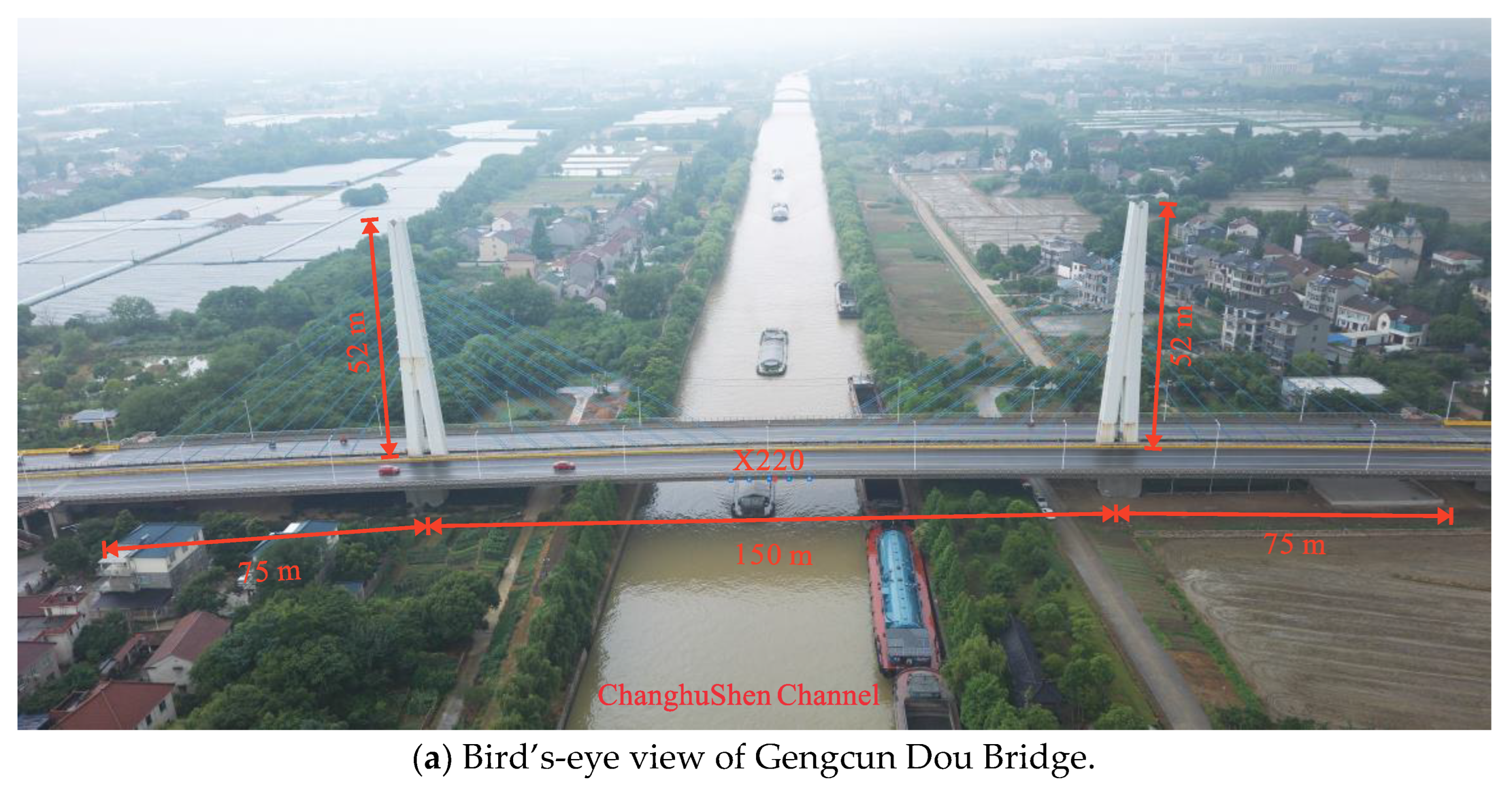
The Gengcun Dou Bridge (Figure 5a) is located in Gengcun, Changxing County, Huzhou City, China, along the Changxing–Lvshan Line (X220), spanning over the ChanghuShen Channel. The main bridge is a double-tower cable-stayed bridge, while the approach bridges at both ends consist of 5 spans of continuous prestressed concrete box girder bridges with equal cross-sections. The total length of the bridge is 608.25 m, with the following span combination: 5 × 30.0 m (north approach bridge) + 75.0 m + 150.0 m + 75.0 m (main bridge) + 5 × 30.0 m (south approach bridge). The main tower is constructed using steel box sections, with dimensions of 3.4 × 7.984 m at the bottom and 2.87 × 2.88 m at the top, standing 52.8 m above the bridge deck. It utilizes longitudinal stiffening ribs and cross-strengthening ribs to ensure stiffness. The completely symmetrical cable system comprises 64 cables arranged in a fan shape, utilizing the parallel wire cable system. The detailed features of the stay cables are presented in Table 1. The main girder of the bridge is designed as a triangular box structure with three chambers, comprising top and bottom plates, diagonal and vertical webs, a cantilever plate, and transverse bulkheads. The net width of the girder is 32.5 m at the top and 4 m at the bottom, with specific thicknesses specified for each component.
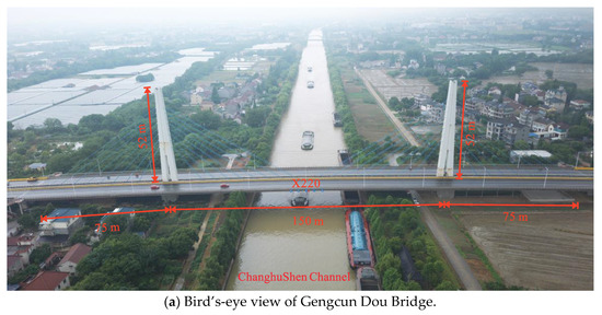
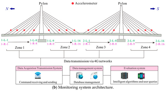
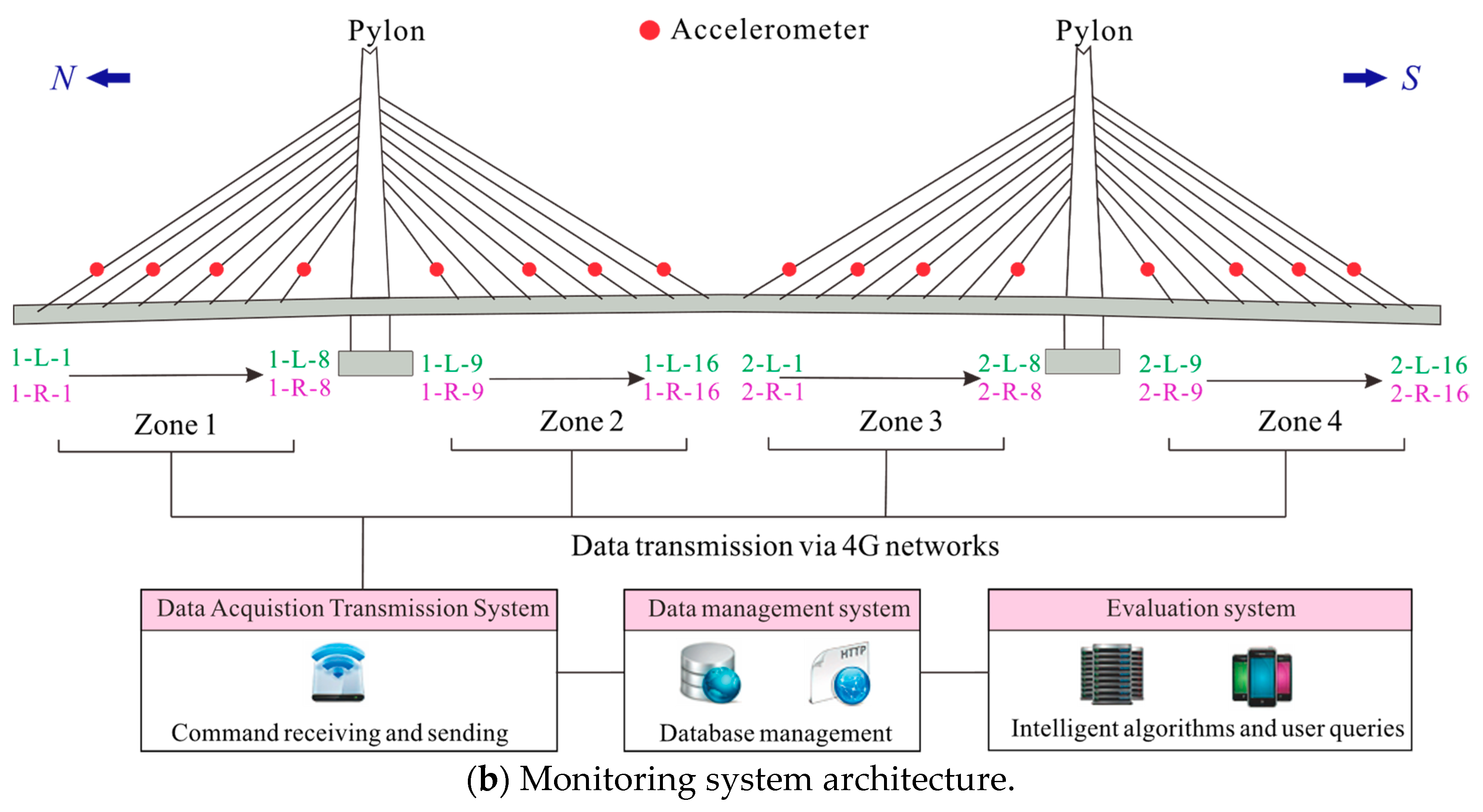
Figure 5.
Gengcun Dou Bridge and its monitoring system.

Table 1.
Geometric feature of stay cables.
To monitor the in-service performance of the stay cable, a layout consisting of 32 accelerometers positioned approximately 3 to 4 m from the bridge deck plate is utilized to monitor changes in the cable force during an operational environment, as illustrated in Figure 5b. Considering the practicality and symmetry of on-site wiring, it is partitioned into four sensing areas, each equipped with 8 accelerometers. These sensors transmit data in real time to the cloud platform for data management via the 4G network data transmission system, enabling the observation of cable force changes and facilitating early warning and periodic structural reliability assessment implementation.
3.2. Monitoring Data Analysis and the Probability Model Establishment
3.2.1. Monitoring Data Analysis
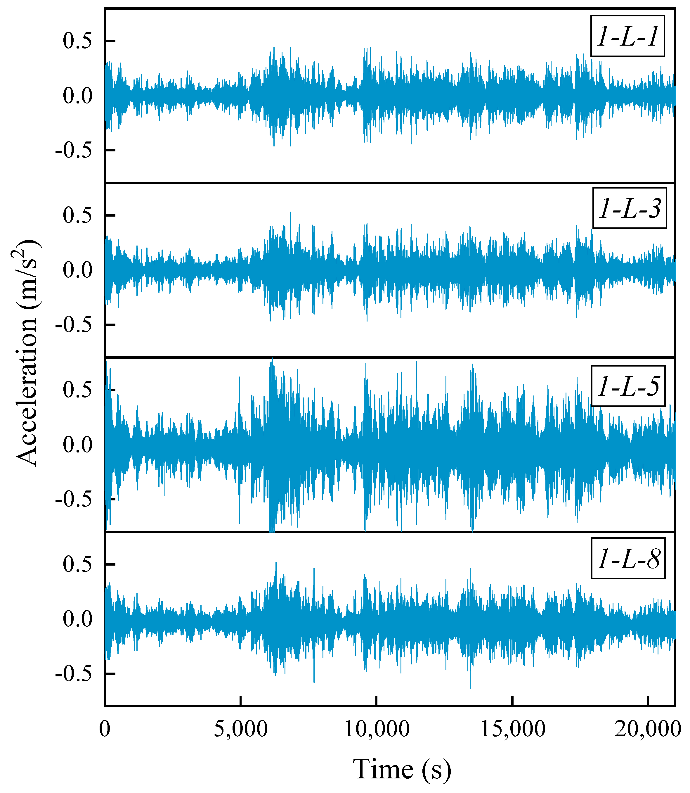
In Figure 6, it is shown that vibration data from the stay cables were collected on the left panel of the northern bridge. It is well established that vibration monitoring data often exhibit faults such as spikes, baseline nonlinear drift, and excessive noise. Thus, vibration data from a fault can significantly impact its spectrum. Further, analyzing unprocessed raw data can significantly distort the facts of structural assessment. Consequently, a range of classical signal pre-processing techniques are employed to process these signals, including low-pass band filtering and outlier rejection, as precursors to FSP. To be more specific, the low-pass band filter was configured with a passband frequency from 0 Hz to 10 Hz and attenuation of 60 dB, following the Nyquist–Shannon sampling theorem and VFM requirements. The accelerometer’s sampling frequency was set at 50 Hz to ensure that the data were properly sampled. By using classical signal pre-processing techniques, the vibration data are filtered to remove outliers and high-frequency component noise that may affect the accuracy of the analysis. This pre-processing step is crucial to ensure that the analysis results are reliable and accurate.
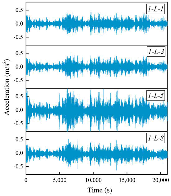
Figure 6.
Acceleration of stay cables at the left panel of the bridge after pre-processing.
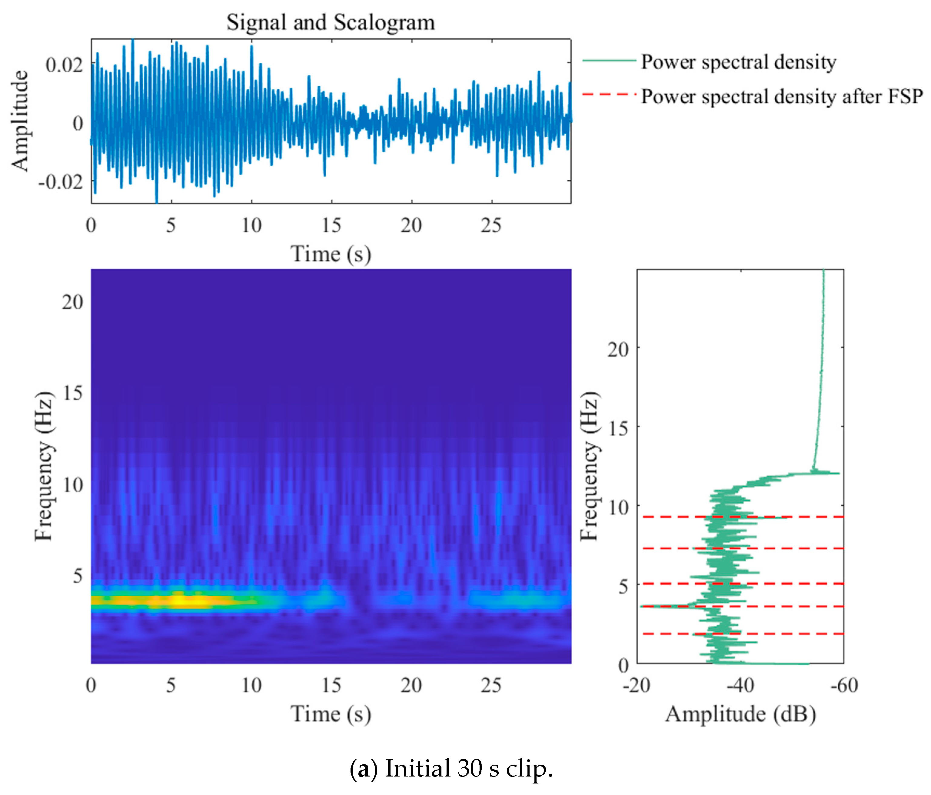
The graphical depiction presented in Figure 7 showcases the results of the time–frequency spectrum post the FSP method. The FSP method is a technique used to improve the readability of signals in the frequency domain. The computational parameters utilized for this study were carefully selected to achieve accurate and reliable results. The step size, a parameter that controls the time resolution of the analysis, was set to 101. The exponentiation order , which controls the frequency resolution, was set to 50. The frequency convergence threshold, which is used to stop the iteration process, was set at a value of . Finally, the total number of iterations was set to 1000. The resultant spectrum demonstrates a high concentration of energy at the accurate position of the natural frequency (red dashed lines in Figure 7). This indicates that the FSP method successfully identified the target frequency with minimal distortion. This feature is crucial in many applications where accurate frequency identification is necessary. In conclusion, the FSP method is a reliable and effective technique for analyzing signals in time and frequency domains. Its ability to reduce distortion in the target frequency pickup makes it highly valuable in many applications, including those in the fields of engineering, physics, and medicine.
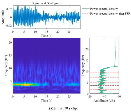
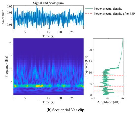
Figure 7.
Time–frequency spectrum of stay cable (No. 1-L-1) after performing FSP.
As can be seen from Figure 7, the operational modes of the stay cable (No. 1-L-1) are identified and present significant peaks at the natural frequency and octave frequencies of the measured cable. The identified frequencies in the initial 30 s clip are 1.90 Hz, 3.64 Hz, 5.07 Hz, 7.3 Hz, and 9.3 Hz, and in the sequential 30 s clip, they are 1.80 Hz, 3.61 Hz, and 9.17 Hz. Therefore, the objective of FSP-VFM is to obtain the frequency interval between two adjacent frequency peaks, which can then be considered the fundamental frequency of the cable for force estimation. Referring back to Equation (2) and the geometric feature of stay cables in Table 1, the fundamental frequency and the corresponding cable force (No. 1-L-1) can be estimated as [1.819 Hz, 4671.7 kN] and [1.813 Hz, 4656.3 kN], respectively. Additionally, in this case, the time interval of 30 s set by the FSP-VFM takes into account the local speed limit of 60 km per hour and the time required to cross the bridge.
3.2.2. Load Effect Modeling
Generally, the probability distribution of the load effect differs from the probability distributions of the individual loads, given that the load effect results from the combination of multiple loads. Furthermore, it is challenging to theoretically derive the probability distribution of the load effect from the probability distributions of the individual loads, especially when each load has a different probability distribution. Consequently, the probability of the load effect was investigated using monitoring data. Structural responses to environmental loads, including wind, temperature, vehicle, and seismic loads, may obscure alterations in structural behavior resulting from genuine structural damage. Hence, it is crucial to employ reliable methodologies for segregating the various loading components from the measured response data, establishing a probabilistic model for the loads, and subsequently deriving dependable results for structural reliability assessment.
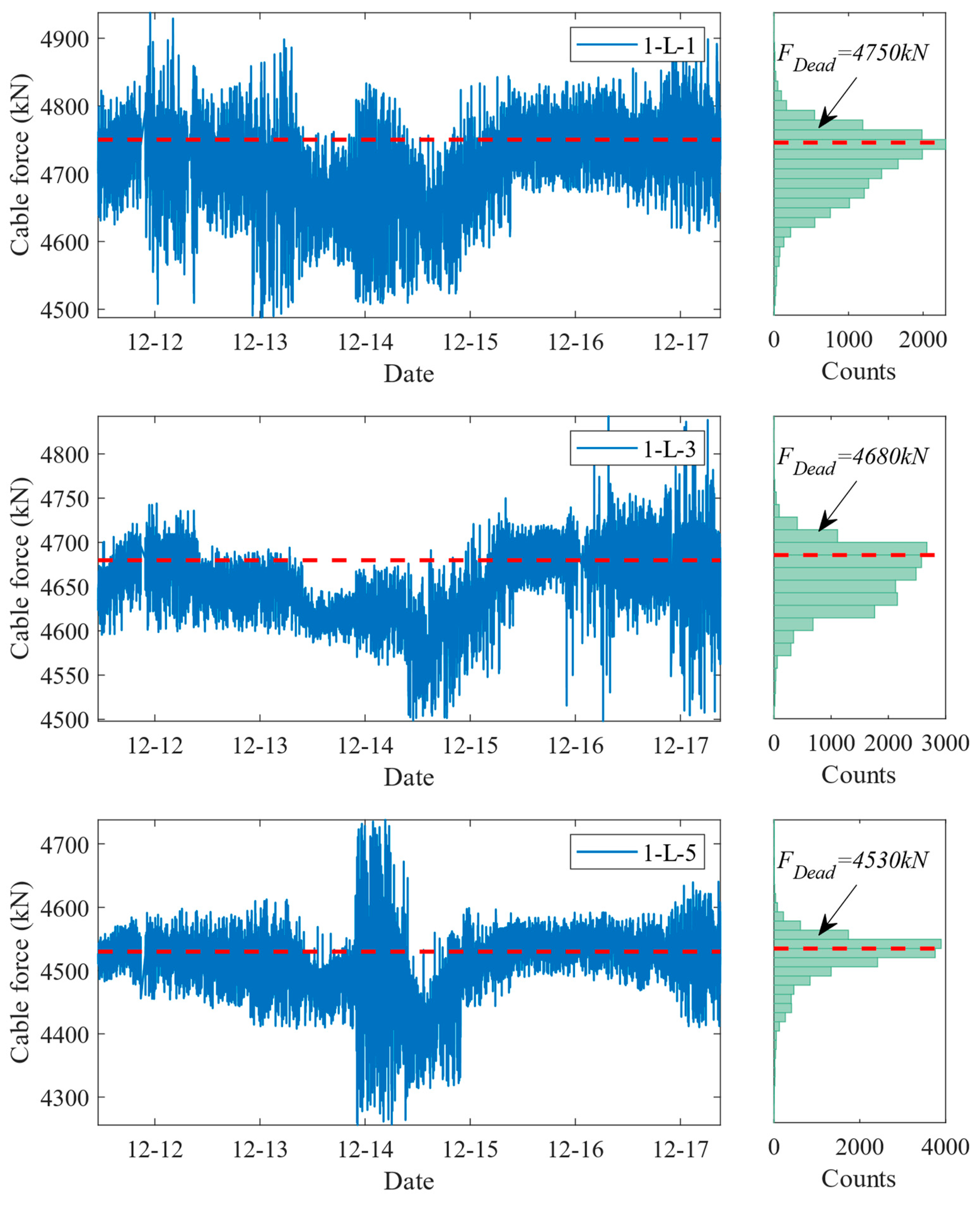
It is widely acknowledged that the total load sources affecting stay cables in service primarily stem from slow-trend and fast-trend sources [41,42,43]. More specifically, fast-trend load sources resulting from cable force changes are predominantly influenced by traffic and wind loads, while slow-trend load sources arising from cable force changes are mainly influenced by temperature and dead-load factors. Figure 8 shows the monitored cable forces (response) and estimated cable forces due to dead loads for a week in service. It is seen from the left-hand panel of Figure 8 that long-term cable forces comprise two components: the slow-trend variation and fast-trend components.
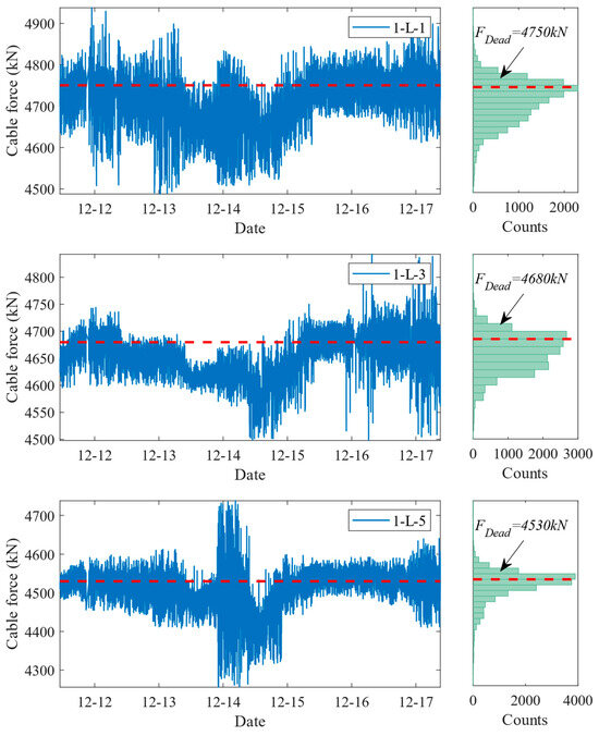
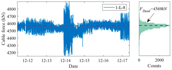
Figure 8.
Identified cable forces and estimation of dead-load-induced cable force.
For the slow-trend variation component, a statistical approach has been developed to ascertain the value of the cable force induced by dead load. The kernel density estimation (KDE) was employed to fit the measured cable force data, depicted in the right-hand panel of Figure 8. The cable force corresponding to the maximum probability density value is then defined as the cable force induced by the dead load [44]. Then, the dead-load-induced cable force can be represented as a constant value, which is utilized in constructing the probability model. The sensitivity of structural components to loads varies, resulting in differing response changes even when subjected to the same load. As a result, various separation methods, such as the moving average method (MAM), empirical mode decomposition (EMD), variational mode decomposition (VMD), and wavelet transform-based techniques, among others, have been proposed to accurately segregate the loading components from the measured response data [45]. Utilizing these separation methods enables the acquisition of precise structural condition assessment results, facilitating informed decisions regarding structural maintenance.
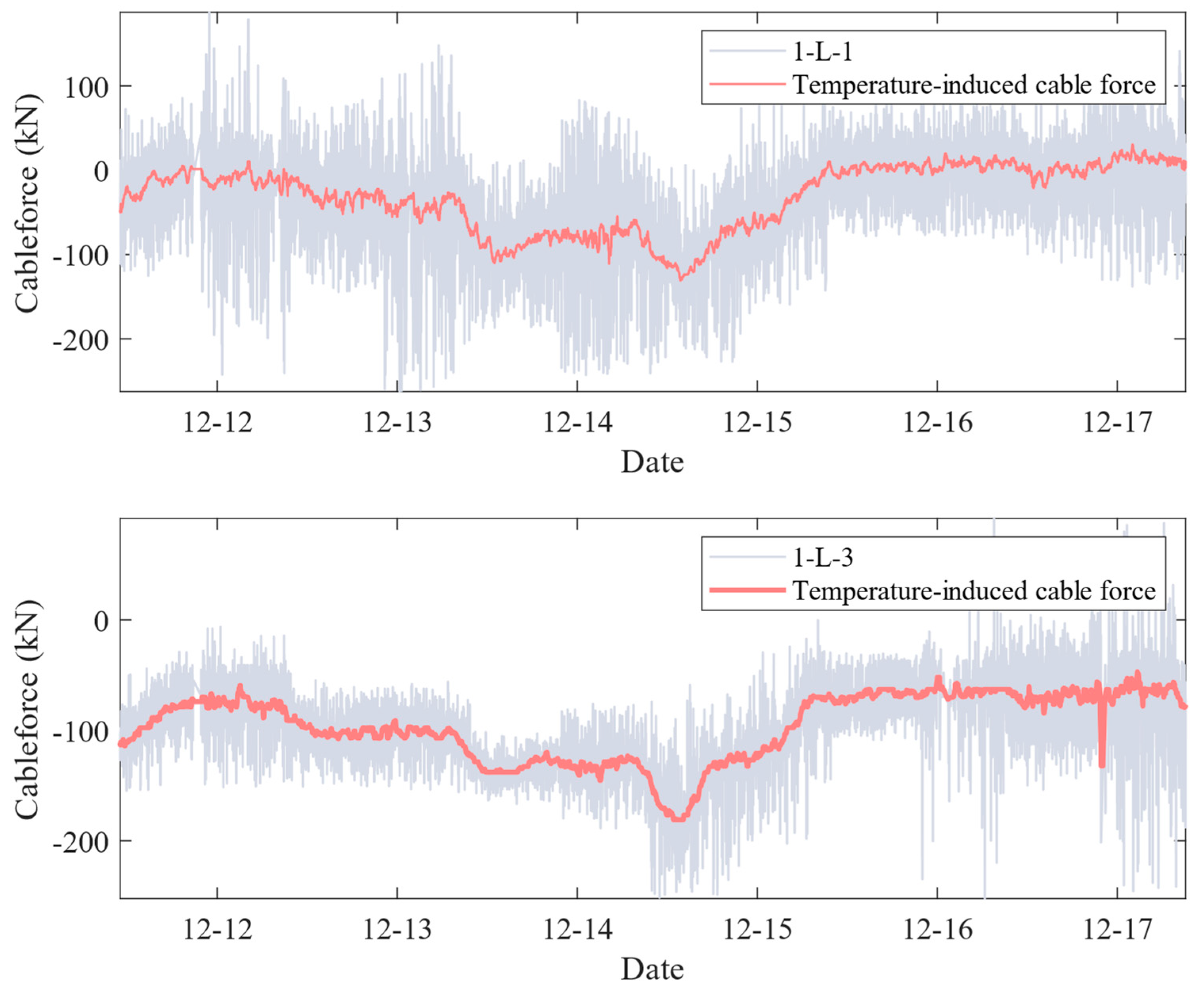
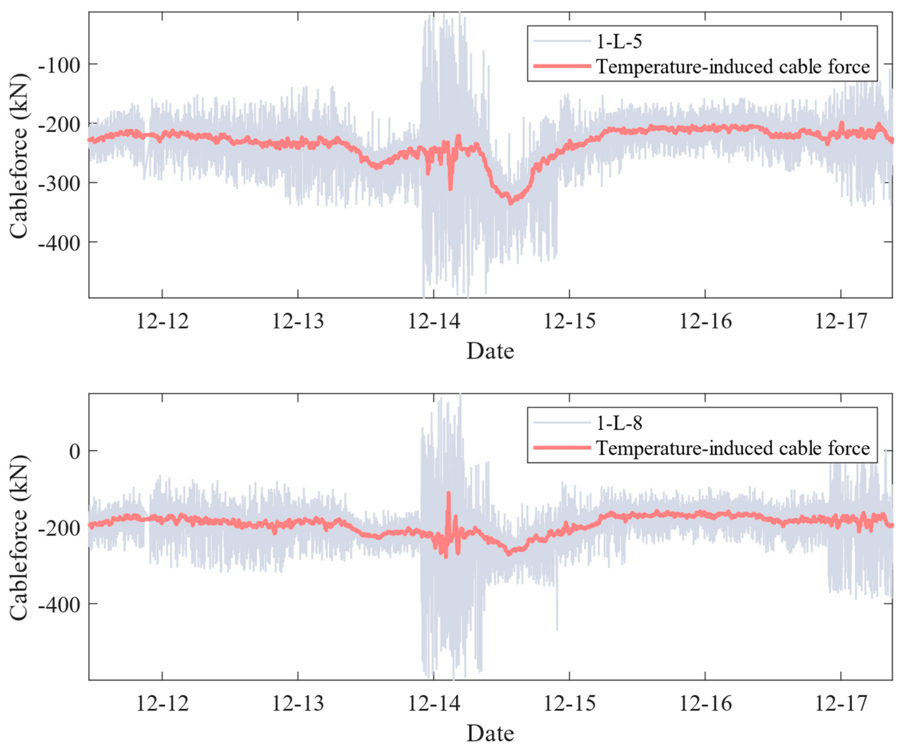
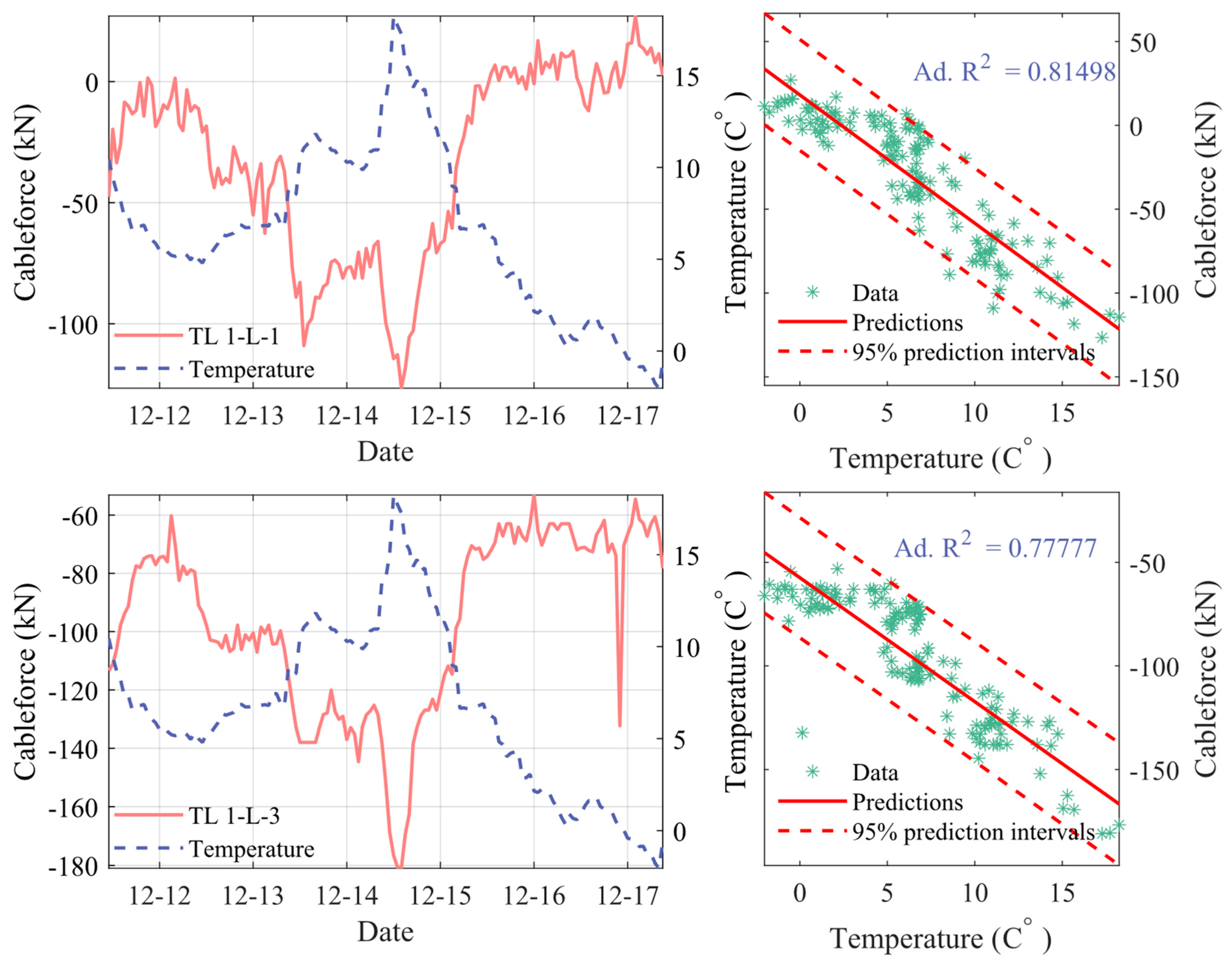
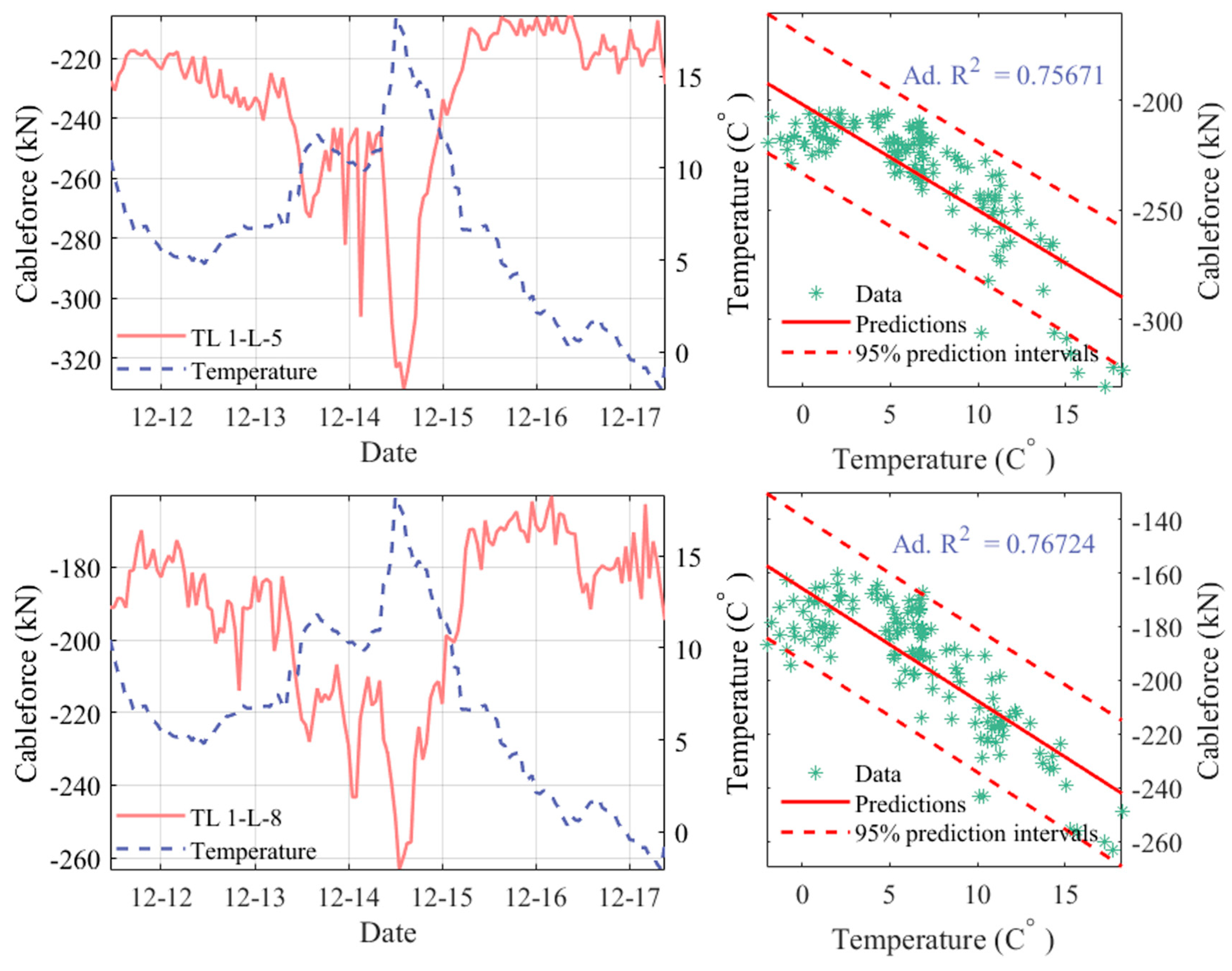
Following the estimation of the dead load, the moving average method (MAM) is employed to isolate the cable force induced by temperature effects from the monitored cable load (identification by FSP-VFM). In the absence of in-site temperature sensors situated within the cables, air temperature data from a weather station located 300 m directly north of the Gengcun Dou Bridge were utilized to validate this load separation method. Figure 9 displays the results of thermal response separation, with the red line representing the slow-trend component and the gray line representing the cable force identified after eliminating the constant dead load. Figure 10 shows the average temperature history (blue dotted line) for 12 December 2023 and 17 December 2023, recorded hourly at the weather station for comparison with the slowly varying components extracted in Figure 9. The peaks of the cable force–temperature pairs were observed between 15:00 and 16:00 each day, with the adjusted R-squared (correlation coefficients) ranging from 0.75 to 0.8. The observed variation may be attributed to static loads on the bridge, specifically static wind loads and temperature-induced loads, indicating a trend consistent with findings in the literature [46].
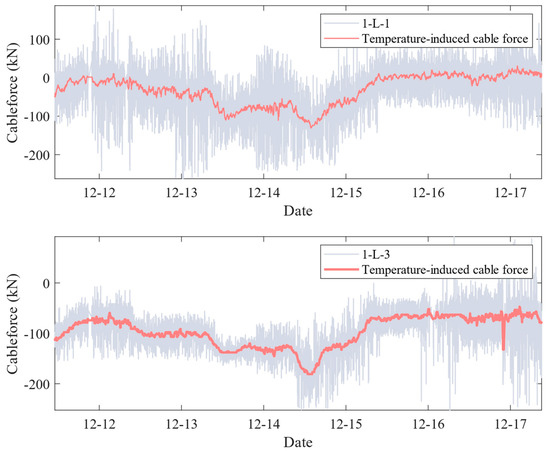
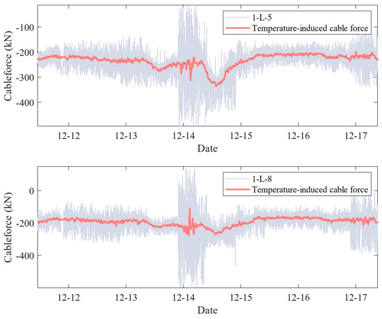
Figure 9.
Result of thermal response separation.
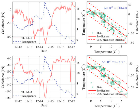
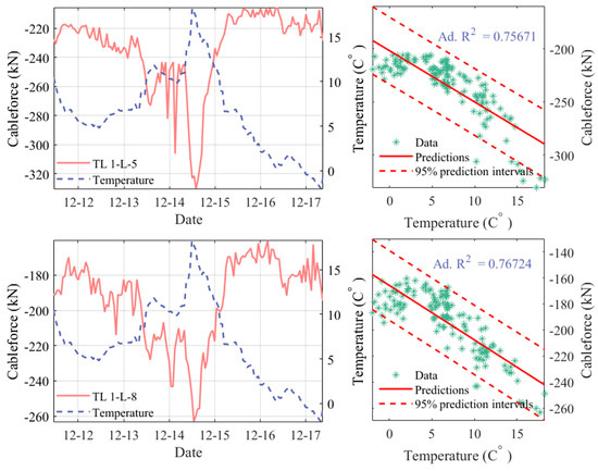
Figure 10.
Correlation between the temperature-induced cable force and the air temperature.
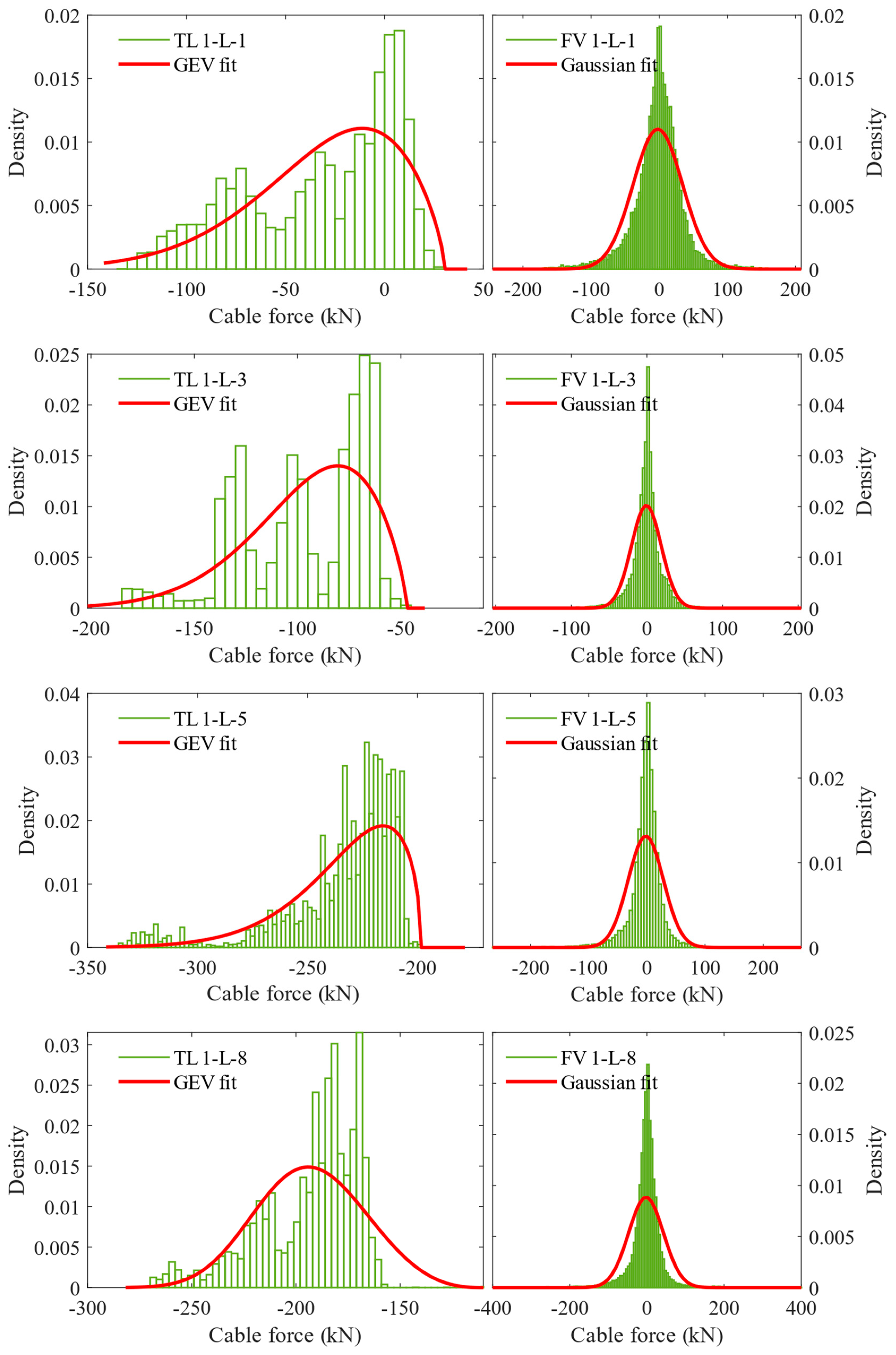
Subsequently, following the removal of the slow-varying trends of the cable force responses using MAM, the remaining components, referred to as the dynamic responses (fast-varying component), were utilized to represent the dynamic loading effects of traffic and wind. The probability density distributions of the slow-varying component and the fast-varying component are illustrated in Figure 11. Additionally, the PDF of the generalized extreme value (GEV) distribution with a location parameter , scale parameter , and shape parameter , and a one-dimensional Gaussian distribution with mean parameter and standard deviation , is expressed as follows:
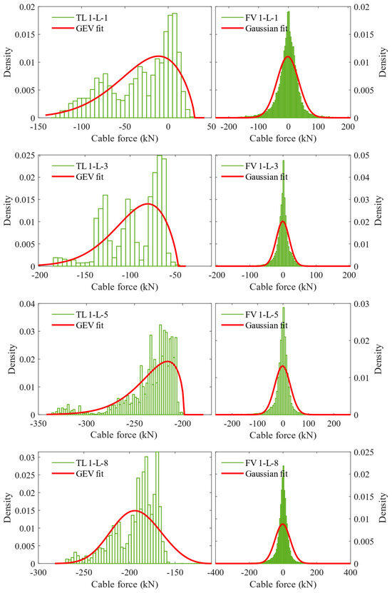
Figure 11.
Probability model of temperature-induced cable force (slow trend) and fast-trend cable force.
The results indicate considerable variation in the probability distributions of cable forces among different cables, despite similar loading conditions. Notably, the probability distribution of cable force differs between short and long tension cables. This demonstrates that the PDF value of the stay cable force is influenced by applied loads, geometric features, and boundary conditions, which aligns with the research recommendations of [47]. In summary, the probability model establishment for load effects was established and is described in Table 2, in preparation for reliability analysis.
Table 2.
Probability distributions of the load effects.
3.3. Reliability Assessment of Stay Cables
The Gengcun Dou Bridge exemplifies a standard prestressed concrete cable-stayed bridge, wherein flexible cables serve as the fundamental force elements. The primary mechanism of this structure entails achieving a prudent distribution of initial internal forces to guarantee structural rigidity. Given the possible decrease in load-carrying capacity and lifespan of the structural cables due to environmental erosion, material degradation, and fatigue damage during operation and maintenance, it becomes imperative to monitor the force characteristics of the cable members to assess the structural reliability.
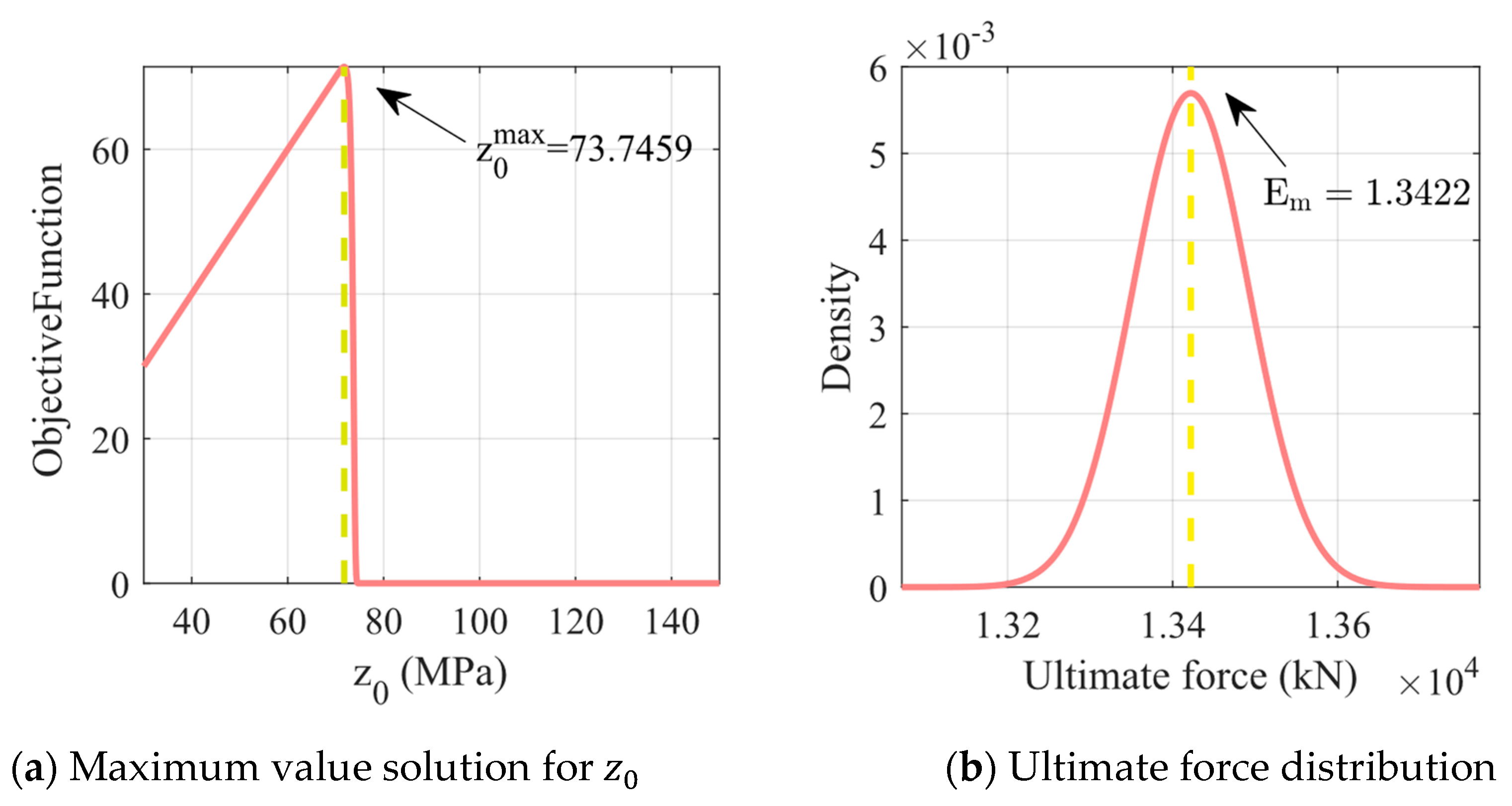
Notably, Section 2.3 considers uncertainties associated with strength properties to adequately describe the resistance properties of the stayed bridges at Gengcun Dou Bridges. The stay cables are all of the size of PESM 7-187 (). In testing, a batch of high-tensile steel wires with a wire length of 500 mm was tested in 15 groups. Given that the specimen steel wires are of the same length and shorter, the scale parameter was set to 1. Referring to Equation (12), we obtained a solution satisfying the extreme value problem, resulting in a Weibull distribution shape parameter of 73.7459 kN and a scale parameter of 194.90 kN, as shown in Figure 12a. By combining Equations (8) and (9), we derived the mean value of the ultimate load-carrying capacity of the whole cable as 13,422 kN, with a standard deviation of 70.04 kN, as shown in Figure 12b.

Figure 12.
Testing results of resistance properties of PESM 7-187.
As noted earlier, fatigue and corrosion are the main concerns for stay cables, leading to varying degrees of deterioration. In the actual resistance strength assessment process, both non-destructive and destructive testing methods, such as the open window method, should be employed to investigate the structural condition of each cable, including assessing for wire breakage and corrosion. However, due to the lack of inspection information, the degradation model with coupled corrosion–fatigue introduced in Section 2.3 is adopted as the resistance probability model, expressed as
where the first term represents the deterioration factor under coupled corrosion–fatigue influence, while the second term represents the influence factor of the material itself.
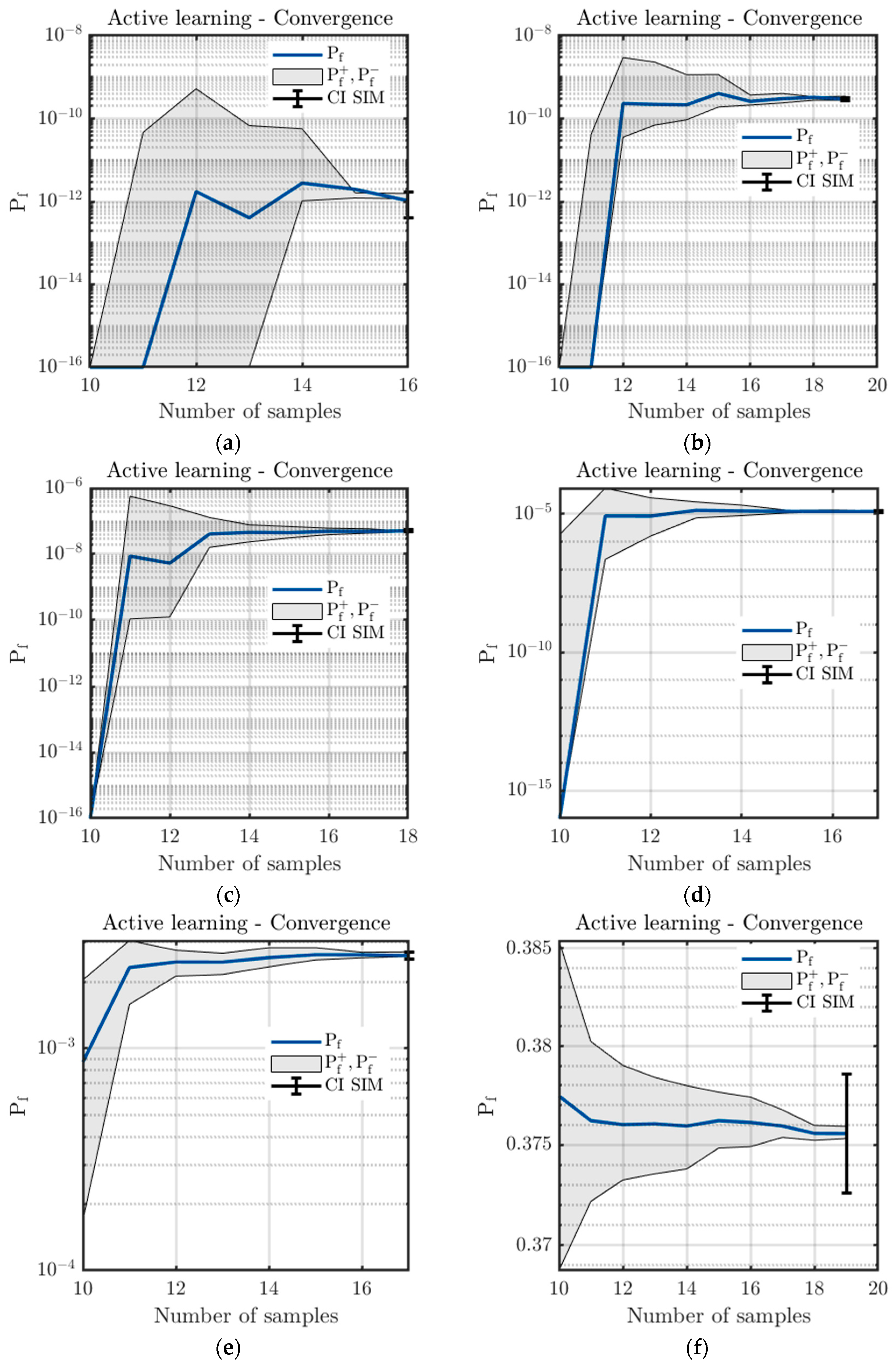
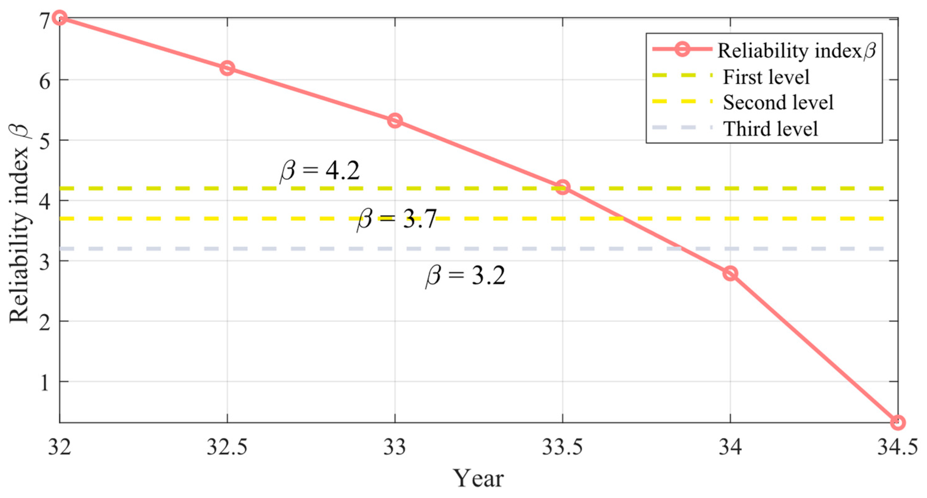
Figure 13 illustrates the reliability analysis results of the GP model-based method for 1-L-1. The GP model-based adaptive method relies on iteratively constructing models that approximate the limit-state function. These surrogates are adaptively refined by incorporating limit-state function evaluations into their experimental designs until a suitable convergence criterion is reached, related to the accuracy of the probability of failure. As depicted in Figure 13a–f, the probability of failure experiences a rapid increase from to . When the service time is less than 33 years, the probability of failure under corrosion–fatigue influence is not greater than regardless of whether or not flow growth is considered. Consequently, despite the absence of specific resistance test results, the fatigue reliability indices do not decrease to a level sufficient to compromise the overall integrity of the cable-stayed bridge. These findings offer a valid assessment of the ultimate load-carrying capacity of a single tension cable solely based on the measurement of the micro-vibration information of the cable. Similarly, for comparison, the reliability index of the stay cables was calculated. The change in the reliability index over a service period of 0 to 40 years is calculated on a half-yearly basis. The results in Figure 14 only depict the interval of significant changes in reliability occurring between the 32nd and 34th years of service. Based on the current monitoring information, it can be inferred that the reliability surpasses 4.2 when the service period reaches the 33rd year, thus meeting the reliability requirement stipulated for structural members at the Grade 1 safety level in the Chinese code (GB50068, [48]). In other words, it meets the reliability requirement specified in the Chinese code for structural components at the Class I safety level. As the service time gradually increases, the reliability index sharply decreases. By the 34th year of service, the reliability falls below the minimum requirement for safety levels. In summary, this information will assist bridge owners in making informed decisions regarding bridge maintenance, and provide bridge engineers with detailed data to support their decision-making processes.
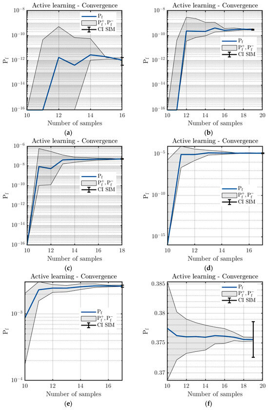
Figure 13.
Estimation result of failure probability for stay cable 1-L-1: (a) 32 years; (b) 32.5 years; (c) 33 years; (d) 33.5 years; (e) 34 years; (f) 34.5 years.
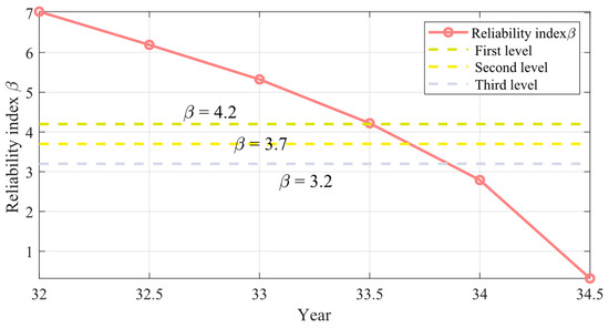
Figure 14.
Estimation result of reliability index β for stay cable 1-L-1.
4. Conclusions
This paper presented a case study on the active learning reliability assessment of the stay cables of the Gengcun Dou Bridge, utilizing monitoring data recorded by the structural health monitoring (SHM) system. The proposed strategy involved cable force identification using the frequency-squeezing processing (FSP) technique within the vibration frequency method (VFM), statistical analysis of load effects on stay cables, and the implementation of a Gaussian process-based surrogate model for estimating failure probability. This study concluded with several significant findings.
Beginning with the classical method of identifying cable force, this paper analyzed a novel approach for identifying cable force in bridge cable members within a micro-vibration environment. By integrating the vibration method and establishing FSP, the study elucidated the relationship between frequency and cable force, reduced uncertainty in selecting the base frequency of cable force, and established a clear and intuitive mapping relationship between cable force and frequency. These findings were conducive to long-term, real-time cable force analysis.
Probabilistic models were developed for the degradation of ultimate load capacity and the load effect based on Daniel’s model and monitoring data, respectively. This resistance degradation model, which accounted for the coupling effect of corrosion and fatigue, recommended the Gaussian distribution. The moving average method (MAM) was used to classify the load effects and model the probability of slow- and fast-trend effects. The generalized extreme value (GEV) distribution model was recommended for slow-trend effects, whereas the Gaussian distribution model was recommended for fast-trend effects. The modeling results demonstrated that the stay cables in Gengcun Dou Bridges could be characterized with effective uncertainty properties using the proposed approach, which could also be extended to similar parallel wire cable systems.
Finally, we investigated the use of an active learning strategy for dynamic reliability assessment by employing the Gaussian process-based surrogate model. Information extracted from monitoring data was synthesized to provide staged assessment results. These results serve as valuable references for the design, construction, operation, and maintenance of fatigue–corrosion-resistant bridges. Additionally, they enhance our understanding of the operational conditions of these bridges in terms of suitability, strength, and reliability.
Author Contributions
Conceptualization, H.-X.L. and G.L.; methodology, H.-X.L.; software, G.L.; validation, Y.C., W.F. and B.L.; formal analysis, H.-X.L.; investigation, Y.C.; resources, Y.C.; data curation, W.F.; writing—original draft preparation, H.-X.L.; writing—review and editing, G.L.; visualization, H.-X.L.; supervision, Y.C.; project administration, Y.C.; funding acquisition, W.M. All authors have read and agreed to the published version of the manuscript.
Funding
This work was supported by the Zhejiang Provincial Key Research and Development Program (2021C03154) and the National Natural Science Foundation of China (Grant Nos. 51878235, 51778568, 51578491).
Data Availability Statement
The original contributions presented in the study are included in the article, further inquiries can be directed to the corresponding author.
Conflicts of Interest
Author Yi Chen was employed by the company Zhejiang Communications Construction Group Co., Ltd. Author Bingchun Li was employed by the company Zhejiang Huifeng Construction Engineering Testing Co., Ltd. The remaining authors declare that the research was conducted in the absence of any commercial or financial relationships that could be construed as a potential conflict of interest.
References
- Yang, L.; Ye, M.; Huang, Y.; Dong, J. Study on Mechanical Properties of Displacement-Amplified Mild Steel Bar Joint Damper. Iran. J. Sci. Technol. Trans. Civ. Eng. 2023, 1–14. [Google Scholar] [CrossRef]
- Luo, Y.; Liu, X.; Chen, F.; Zhang, H.; Xiao, X. Numerical Simulation on Crack–Inclusion Interaction for Rib-to-Deck Welded Joints in Orthotropic Steel Deck. Metals 2023, 13, 1402. [Google Scholar] [CrossRef]
- Luo, Y.; Liao, P.; Pan, R.; Zou, J.; Zhou, X. Effect of Bar Diameter on Bond Performance of Helically Ribbed GFRP Bar to UHPC. J Build. Eng. 2024, 91, 109577. [Google Scholar] [CrossRef]
- Li, H.; Zhang, F.; Jin, Y. Real-Time Identification of Time-Varying Tension in Stay Cables by Monitoring Cable Transversal Acceleration. Struct. Control Health Monit. 2014, 21, 1100–1117. [Google Scholar] [CrossRef]
- Kmet, S.; Tomko, M.; Brda, J. Time-Dependent Analysis of Cable Trusses Part II. Simulation-Based Reliability Assessment. Struct. Eng. Mech. 2011, 38, 171–193. [Google Scholar] [CrossRef]
- Xiong, W.; Xiao, R.; Deng, L.; Cai, C. Methodology of Long-Term Real-Time Condition Assessment for Existing Cable-Stayed Bridges. Adv. Struct. Eng. 2010, 13, 111–125. [Google Scholar] [CrossRef]
- Zheng, Y.; Zhang, Y.; Lin, J. BIM–Based Time-Varying System Reliability Analysis for Buildings and Infrastructures. J. Bridge Eng. 2023, 76, 106958. [Google Scholar] [CrossRef]
- Zhou, Y.; Chen, S. Time-Progressive Dynamic Assessment of Abrupt Cable-Breakage Events on Cable-Stayed Bridges. J. Build. Eng. 2014, 19, 159–171. [Google Scholar] [CrossRef]
- Zhang, J.; Chen, K.J.; Zeng, Y.P.; Yang, Z.Y.; Zheng, S.X.; Jia, H.Y. Seismic Reliability Analysis of Cable-Stayed Bridges Subjected to Spatially Varying Ground Motions. Int. J. Struct. Stab. Dyn. 2021, 21, 2150094. [Google Scholar] [CrossRef]
- Zhou, Y.; Chen, S. Reliability Assessment Framework of the Long-Span Cable-Stayed Bridge and Traffic System Subjected to Cable Breakage Events. J. Bridge Eng. 2017, 22, 04016133. [Google Scholar] [CrossRef]
- Wang, C.; Beer, M.; Ayyub, B.M. Time-Dependent Reliability of Aging Structures: Overview of Assessment Methods. ASCE-ASME J. Risk Uncertain. Eng. Syst. Part A Civ. Eng. 2021, 7, 03121003. [Google Scholar] [CrossRef]
- Li, J.X.; Yi, T.H.; Qu, C.X.; Li, H.N.; Liu, H. Adaptive Identification of Time-Varying Cable Tension Based on Improved Variational Mode Decomposition. J. Bridge Eng. 2022, 27, 04022064. [Google Scholar] [CrossRef]
- Fan, Z.Y.; Huang, Q.; Ren, Y.; Zhu, Z.Y.; Xu, X. A Cointegration Approach for Cable Anomaly Warning Based on Structural Health Monitoring Data: An Application to Cable-Stayed Bridges. Adv. Struct. Eng. 2020, 23, 2789–2802. [Google Scholar] [CrossRef]
- Dan, D.; Zeng, G.; Pan, R.; Yin, P. Block-Wise Recursive Sliding Variational Mode Decomposition Method and Its Application on Online Separating of Bridge Vehicle-Induced Strain Monitoring Signals. Mech. Syst. Signal Process. 2023, 198, 110389. [Google Scholar] [CrossRef]
- Zhang, H.; Aoues, Y.; Lemosse, D.; Bai, H.; De Cursi, E.S. Time-Variant Reliability-Based Optimization with Double-Loop Kriging Surrogates. In Proceedings of the 5th International Symposium on Uncertainty Quantification and Stochastic Modeling: Uncertainties 2020; Springer: Berlin/Heidelberg, Germany, 2021; pp. 436–446. [Google Scholar]
- Afshari, S.S.; Pourtakdoust, S.H. Probability Density Evolution for Time-Varying Reliability Assessment of Wing Structures. Aviation 2018, 22, 45–54. [Google Scholar] [CrossRef]
- Yang, N.; Li, J.; Xu, M.; Wang, S. Real-Time Identification of Time-Varying Cable Force Using an Improved Adaptive Extended Kalman Filter. Sensors 2022, 22, 4212. [Google Scholar] [CrossRef] [PubMed]
- Yu, X.; Dan, D. Real-Time Cable Force Identification Based on Block Recursive Capon Spectral Estimation Method. Measurement 2023, 213, 112664. [Google Scholar] [CrossRef]
- Zhang, H.; Zhou, Y.; Huang, Z.; Shen, R.; Wu, Y. Multiparameter Identification of Bridge Cables Using XGBoost Algorithm. J. Bridge Eng. 2023, 28, 04023016. [Google Scholar] [CrossRef]
- Zhu, W.; Teng, W.; Liu, F.; Wu, D.; Wu, Y. Measurement of Cable Force through a Fiber Bragg Grating-Type Thin Rod Vibration Sensor and Its Application. Sensors 2022, 22, 8081. [Google Scholar] [CrossRef]
- Wu, W.H.; Chen, C.C.; Lin, S.L.; Lai, G. A Real-Time Monitoring System for Cable Tension with Vibration Signals Based on an Automated Algorithm to Sieve out Reliable Modal Frequencies. Struct. Control Health Monit. 2023, 2023, 9343343. [Google Scholar] [CrossRef]
- Shafighfard, T.; Kazemi, F.; Bagherzadeh, F.; Mieloszyk, M.; Yoo, D.Y. Chained Machine Learning Model for Predicting Load Capacity and Ductility of Steel Fiber–Reinforced Concrete Beams. Comput.-Aided Civ. Infrastruct. Eng. 2024. [Google Scholar] [CrossRef]
- Asgarkhani, N.; Kazemi, F.; Jakubczyk-Gałczyńska, A.; Mohebi, B.; Jankowski, R. Seismic Response and Performance Prediction of Steel Buckling-Restrained Braced Frames Using Machine-Learning Methods. Eng. Appl. Artif. Intell. 2024, 128, 107388. [Google Scholar] [CrossRef]
- Zheng, P.; Wang, C.; Zong, Z.; Wang, L. A New Active Learning Method Based on the Learning Function U of the AK-MCS Reliability Analysis Method. Eng. Struct. 2017, 148, 185–194. [Google Scholar]
- She, A.; Wang, L.; Peng, Y.; Li, J. Structural Reliability Analysis Based on Improved Wolf Pack Algorithm AK-SS. Structures 2023, 57, 105289. [Google Scholar] [CrossRef]
- Zhang, C. The Active Rotary Inertia Driver System for Flutter Vibration Control of Bridges and Various Promising Applications. Sci. China Technol. Sci. 2023, 66, 390–405. [Google Scholar] [CrossRef]
- Ehre, M.; Papaioannou, I.; Sudret, B.; Straub, D. Sequential Active Learning of Low-Dimensional Model Representations for Reliability Analysis. SIAM J. Sci. Comput. 2022, 44, B558–B584. [Google Scholar] [CrossRef]
- Marrel, A.; Iooss, B. Probabilistic Surrogate Modeling by Gaussian Process: A Review on Recent Insights in Estimation and Validation. Reliab. Eng. Syst. Saf. 2024, 110094. [Google Scholar] [CrossRef]
- Nannapaneni, S.; Hu, Z.; Mahadevan, S. Uncertainty Quantification in Reliability Estimation with Limit State Surrogates. Struct. Multidiscip. Optim. 2016, 54, 1509–1526. [Google Scholar] [CrossRef]
- Zhang, L.; Qiu, G.; Chen, Z. Structural Health Monitoring Methods of Cables in Cable-Stayed Bridge: A Review. Measurement 2021, 168, 108343. [Google Scholar] [CrossRef]
- Yu, X.; Dan, D. Block-Wise Recursive APES Aided with Frequency-Squeezing Postprocessing and the Application in Online Analysis of Vibration Monitoring Signals. Mech. Syst. Signal Process. 2022, 162, 108063. [Google Scholar] [CrossRef]
- Chen, Y.; Zheng, X.; Luo, Y.; Shen, Y.; Xue, Y.; Fu, W. An Approach for Time Synchronization of Wireless Accelerometer Sensors Using Frequency-Squeezing-Based Operational Modal Analysis. Sensors 2022, 22, 4784. [Google Scholar] [CrossRef]
- Faber, M.H.; Engelund, S.; Rackwitz, R. Aspects of Parallel Wire Cable Reliability. Struct. Saf. 2003, 25, 201–225. [Google Scholar] [CrossRef]
- Mao, J.X.; Wang, H.; Li, J. Fatigue Reliability Assessment of a Long-Span Cable-Stayed Bridge Based on One-Year Monitoring Strain Data. J. Bridge Eng. 2019, 24, 05018015. [Google Scholar] [CrossRef]
- Hou, N.; Sun, L.; Chen, L. Cable Reliability Assessments for Cable-Stayed Bridges Using Identified Tension Forces and Monitored Loads. J. Bridge Eng. 2020, 25, 05020003. [Google Scholar] [CrossRef]
- Rasmussen, C.E.; Williams, C.K.I. Gaussian Processes for Machine Learning. In Adaptive Computation and Machine Learning; MIT Press: Cambridge, MA, USA, 2008; ISBN 978-0-262-18253-9. [Google Scholar]
- Melchers, R.E.; Beck, A.T. Structural Reliability Analysis and Prediction, 3rd ed.; Wiley: Hoboken, NJ, USA, 2018; ISBN 978-1-119-26607-5. [Google Scholar]
- Moustapha, M.; Marelli, S.; Sudret, B. A Generalized Framework for Active Learning Reliability: Survey and Benchmark. arXiv 2021, arXiv:2106.01713. [Google Scholar]
- Moustapha, M.; Marelli, S.; Sudret, B. Active Learning for Structural Reliability: Survey, General Framework and Benchmark. Struct. Saf. 2022, 96, 102174. [Google Scholar] [CrossRef]
- Echard, B.; Gayton, N.; Lemaire, M. AK-MCS: An active learning reliability method combining Kriging and Monte Carlo simulation. Struct. Saf. 2011, 33, 145–154. [Google Scholar] [CrossRef]
- Teixeira, R. Adaptive Approaches in Metamodel-Based Reliability Analysis: A Review. Struct. Saf. 2021, 89, 102019. [Google Scholar] [CrossRef]
- Deng, Y.; Liu, Y.; Chen, S. Long-Term In-Service Monitoring and Performance Assessment of the Main Cables of Long-Span Suspension Bridges. Sensors 2017, 17, 1414. [Google Scholar] [CrossRef] [PubMed]
- Ding, Y.; Ye, X.W.; Guo, Y. Data Set from Wind, Temperature, Humidity and Cable Acceleration Monitoring of the Jiashao Bridge. J. Civ. Struct. Health Monit. 2023, 13, 579–589. [Google Scholar] [CrossRef]
- Li, H.; Li, S.; Ou, J.; Li, H. Reliability Assessment of Cable-Stayed Bridges Based on Structural Health Monitoring Techniques. Struct. Infrastruct. Eng. 2012, 8, 829–845. [Google Scholar] [CrossRef]
- Ren, Y.; Xu, X.; Huang, Q.; Zhao, D.-Y.; Yang, J. Long-Term Condition Evaluation for Stay Cable Systems Using Dead Load–Induced Cable Forces. Adv. Struct. Eng. 2019, 22, 1644–1656. [Google Scholar] [CrossRef]
- Luo, Y.; Fu, W.; Wan, H.P.; Shen, Y. Load-Effect Separation of a Large-Span Prestressed Structure Based on an Enhanced EEMD-ICA Methodology. J. Struct. Eng. 2022, 148, 04021288. [Google Scholar] [CrossRef]
- Li, J.X.; Yi, T.H.; Qu, C.X.; Li, H.N.; Liu, H. Early Warning for Abnormal Cable Forces of Cable-Stayed Bridges Considering Structural Temperature Changes. J. Bridge Eng. 2023, 28, 04022137. [Google Scholar] [CrossRef]
- GB50068; Load Code for the Design of Building Structures. Ministry of Housing and Urban-Rural Development of the People’s Republic of China; China Architecture & Building Press: Beijing, China, 2018.


Disclaimer/Publisher’s Note: The statements, opinions and data contained in all publications are solely those of the individual author(s) and contributor(s) and not of MDPI and/or the editor(s). MDPI and/or the editor(s) disclaim responsibility for any injury to people or property resulting from any ideas, methods, instructions or products referred to in the content. |
© 2024 by the authors. Licensee MDPI, Basel, Switzerland. This article is an open access article distributed under the terms and conditions of the Creative Commons Attribution (CC BY) license (https://creativecommons.org/licenses/by/4.0/).