Research on Collision Restitution Coefficient Based on the Kinetic Energy Distribution Model of the Rocking Rigid Body within the System of Mass Points

Abstract

Rocking structures exhibit significant collapse resistance during earthquakes. In studies of rocking rigid bodies, the collision restitution coefficient is typically determined based on the classical model of the rocking rigid bodies. However, during the rocking process, the collision restitution coefficient, influenced by the uncontrollable error in collision energy dissipation between the rigid body and the ground, indirectly impacts the final results of the equations of motion. Therefore, the rationality and reliability of the collision restitution coefficient are crucial for seismic analysis of rocking rigid bodies and self-centering members. This paper introduces a phasic energy dissipation and kinetic energy redistribution model specifically designed for the rocking rigid body within the system of mass point. This model divides the collision into three distinct stages, incorporating energy dissipation considerations in the first two stages to calculate the total kinetic energy of the rigid body. In the third stage, the remaining kinetic energy is redistributed to precisely determine the analytical solution for the collision restitution coefficient of an ideal, homogeneous rectangular rigid body during collision. Lastly, the validity and reliability of the proposed model are confirmed through comparisons with experimental data.

1. Introduction

Self-centering structures in engineering and unconstrained tall objects within buildings are susceptible to rocking and collisions during seismic events. The collision process results in energy loss, influenced by numerous factors [1,2]. The aleatory and epistemic uncertainties coming from various sources have significant impacts on the accuracy of risk estimates for structures under dynamic excitations [3,4].

In 1963, Housner [5] introduced the concept of “rocking structure”, drawing from his analysis of the 1952 California earthquake and the 1960 Chilean earthquake. He formulated the classical model of the rocking rigid body [6]. This model has garnered widespread recognition among researchers. Notably, within the realm of resilient seismic design, this model and its analytical methods have undergone notable advancements and enhancements since their inception [6,7].

Beck and Skinner [8] initially explored the utilization of the rocking concept in seismic bridge design in 1974 [9]. Huckelbridge and Clough [10,11] performed shaking table experiments on three- and nine-story rocking steel frame models in 1977, revealing the beneficial role of structural rocking in mitigating the need for increased structural strength and ductility [12]. In 1980, Yim et al. [13] discovered that the rocking response of rigid bodies during earthquakes was highly susceptible to variations in size, slenderness ratio (h/b), and ground motion characteristics. In the same year, Aslam et al. [14] examined the rocking behavior of rigid bodies under earthquake conditions through experimental investigations, concluding that the overturning tendency of rigid bodies is significantly influenced by base parameters, the collision restitution coefficient, and changes in ground motion. In 1981, the South Rangitikei railway bridge in New Zealand became the first to incorporate rocking piers, successfully implementing the rocking structure concept in bridge engineering [15]. Apostolou et al. [16] conducted an analysis of rocking vibration parameters for rigid bodies resting on rigid and linear elastic foundations in 2007, emphasizing the significance of rigid body size, slenderness ratio, and foundation vibration parameters as critical factors influencing overturning [6]. As the concept of “resilient structures” gained popularity, more researchers began exploring the field of rocking structures. In 2009, Mariott et al. [17] introduced a novel method utilizing external energy dissipation devices, as opposed to internal reinforcement, to address the challenge of post-earthquake reinforcement replacement. They validated the effectiveness of these rocking piers through quasi-static and quasi-dynamic testing, demonstrating their superior energy dissipation and self-centering capabilities. Addressing concerns regarding the durability of prestressed bundles and external energy dissipation devices, Guo et al. [18], in 2015, explored the use of basalt fiber-reinforced composite materials, modified aluminum alloys, and glass fiber-reinforced polymer materials for the fabrication of prestressed reinforcements, external dissipation devices, and pier sleeves. They subsequently evaluated the seismic performance of these rocking piers through quasi-static testing. In 2016, the Huangxulu overpass bridge, a self-centering rocking bridge project in China spanning the Jing-Tai Expressway [19,20], implemented a seismic design method based on the displacement of its rocking bridge structure. This development ushered in the era of rocking bridge construction in the 21st century, paralleled by the contemporary construction of the Wigram-Magdala overpass bridge in New Zealand [21,22]. With the increasing application of rocking structures in engineering, researchers have increasingly focused on effectively incorporating seismic reduction principles of rocking structures into practical engineering implementations [23,24,25,26,27,28].

Prior research indicates that the magnitude of the collision restitution coefficient significantly impacts the shape of the overturning region of a rocking rigid body [6], subsequently influencing pertinent studies. Hence, accurate and rational estimation of the collision restitution coefficient holds crucial significance for seismic investigations into rocking structures. Schau et al. [29] conducted a study in 2014 that investigated the rocking motion of rigid bodies subjected to earthquake excitation, utilizing numerical integration of equations of motion and finite element methods. Highlighting that any variations in ideal geometric shapes or contact conditions would result in an increase in the collision restitution coefficient, they proposed a collision restitution coefficient value of 0.8 for rigid bodies exhibiting a slenderness ratio of 2. This value theoretically surpasses the theoretical value of 0.7 employed in classical models. In 2016, Kallionizis et al. [30] compiled a collision restitution coefficient based on previous experiments conducted on rocking rigid bodies. Their findings revealed that for rigid bodies with a small slenderness ratio, the classical model’s collision restitution coefficient exhibits significant discrepancies compared to experimental outcomes. Notably, experimental values consistently exceeded the predictions of the classical theoretical model. Based on their observations, an improved model was proposed, assuming that collisions between the rigid body and the base generate impulses acting specifically between the two bottom corners of the rigid body. While the revised model aligned closely with experimental data, it was noteworthy that the length of the rotational surface was determined empirically [6]. In 2018, Čeh et al. [31] conducted free rocking tests on single rigid bodies, excluding slipping and bouncing. Their findings supported the previous research conclusions of Kallionizis et al. Additionally, they developed an algorithm capable of simulating rigid body rocking. In 2022, Jia et al. [7] conducted shaking table tests on rocking rigid bodies, aiming to investigate their seismic response characteristics. Their measurements revealed an actual collision restitution coefficient of 0.901, exceeding the theoretical value of 0.873 predicted by the classical model of the rocking rigid body.

Considering the present research landscape and its outcomes, the classical model of the rocking rigid body exhibits a significantly high margin of error in its collision restitution coefficient. The primary source of the substantial error lies in the fact that the classical model of the rocking rigid body, while utilizing the conservation of angular momentum for its solutions, disregards the system satisfying conservation of angular momentum as a comprehensive entity encompassing both the rigid body and the ground. Conversely, the advanced models incorporate empirically determined parameters, which lack a theoretical foundation. This paper aims to further refine the rocking structure rigid body model by meticulously analyzing the energy dissipation mechanisms during collisions and introducing a kinetic energy distribution model tailored for rocking rigid bodies within the mass point system. This model divides the collision into three distinct stages, incorporating energy dissipation considerations in the first two stages to calculate the total kinetic energy of the rigid body. In the third stage, the remaining kinetic energy is redistributed under the action of stresses. This approach yields an analytical solution specific to homogeneous regular rectangular rigid bodies. Compared to both experimental data and the classical model, the theoretical values derived from this model exhibit significantly reduced errors, with a correlation coefficient exceeding 0.9. This offers a novel perspective for exploring energy dissipation mechanisms in rocking rigid bodies.

2. Model and Collision Restitution Coefficient

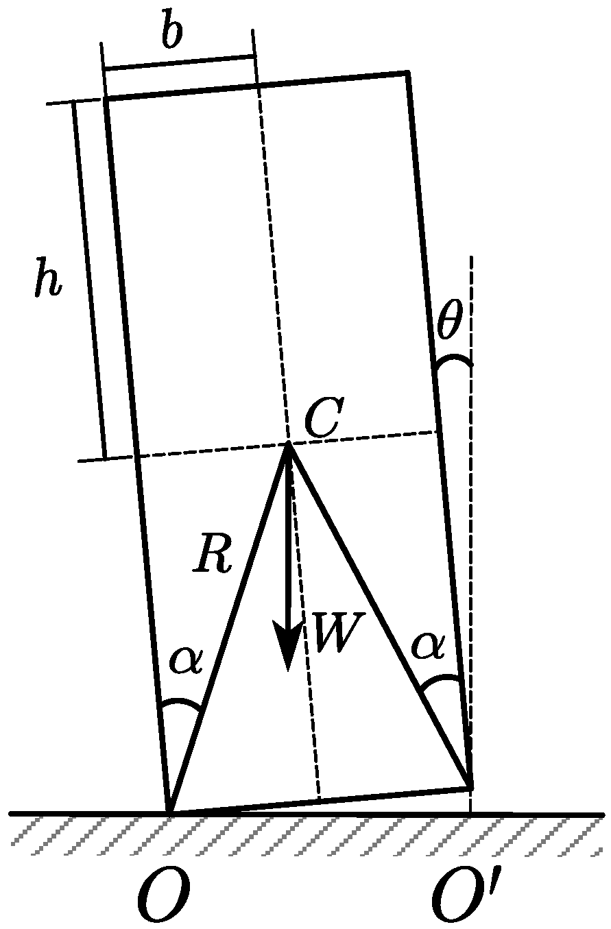
2.1. Classical Model of the Rocking Rigid Body

The classical model of the rocking rigid body was first proposed by Housner [5] in 1963, as shown in Figure 1. The center of gravity of the rigid body is located at point $C$, where $h$ is half the height of the rigid body, and $b$ is half the width of the rigid body. After the initiation of rocking, the rigid body rotates about the pivot points $O$ or $O^{\prime }$ during different time periods.

Here are the assumptions for the classical model of the rocking rigid body [32]:

• The model is simplified for a 2-D geometry;
• The block and the base are rigid;
• The rigid body is a homogeneous rectangular block;
• There is no bouncing or complete lifting of the body;
• Blocks are assumed not to be sliding on the ground or relative to each other;
• Material stiffness and damping are not considered, i.e., the blocks cannot be compressed nor do they store/dissipate elastic energy;
• The collision lasts for an infinitely small time interval;
• The rigid body is not damaged during the collision.

Since the rigid body is a homogeneous and symmetrical structure, the derivation of the collision restitution coefficient in the classical model of the rocking rigid body only considers the instantaneous collision when the rigid body transitions from rotating about point $O$ to rotating about point $O^{\prime }$. The derivation process for the collision restitution coefficient in the classical model of the rocking rigid body is given as follows.

Based on Konig’s theorem of angular momentum, before the collision, the angular momentum of the rigid body about $O^{\prime }$ is the sum of the angular momentum of the rigid body about its center of mass and the angular momentum obtained by concentrating the mass of the rigid body at the center of mass about $O^{\prime }$ [7]. Therefore, the angular momentum of the rigid body about $O^{\prime }$ before the collision is

$$L^{-}=I_C{\dot{\theta }}^{-}+WR{\dot{\theta }}^{-}\sin (\frac{\mathsf{\pi }}{2}-2\alpha )R$$

(1)

where $I_C$ represents the angular momentum of the rigid body about its center of mass, ${\dot{\theta }}^{-}$ is the angular velocity of the rigid body before the collision, $W$ is the total mass of the rigid body, $R$ is the semi-diagonal of the rigid body, and $\alpha$ is the angle between the semi-diagonal and the height side of the rigid body.

By applying the equation for $I_O=I_C+W{R}^2$ and trigonometric relationships, the angular momentum of the rigid body about $O^{\prime }$ before the collision can be simplified to

$$L^{-}=I_O{\dot{\theta }}^{-}-2W{b}^2{\dot{\theta }}^{-}$$

(2)

where $I_O$ is the angular momentum of the rigid body about point $O$.

The angular momentum after the collision is

$$L^{+}=I_{O^{\prime }}{\dot{\theta }}^{+}$$

(3)

where $I_{O^{\prime }}$ is the angular momentum of the rigid body about point $O^{\prime }$, and ${\dot{\theta }}^{+}$ is the angular velocity of the rigid body after the collision.

According to the conservation of angular momentum, at the instant of collision, the collision restitution coefficient at the instant of collision when the rigid body transitions from rotating about point $O$ to rotating about point $O^{\prime }$ can be obtained as

$$r=\frac{{\dot{\theta }}^{+}}{{\dot{\theta }}^{-}}=\frac{I_O-2W{b}^2}{I_{O^{\prime }}}$$

(4)

Since the rigid body is a homogeneous rectangular rigid body, $I_O=I_{O^{\prime }}=\frac{4}{3}W{R}^2$, the collision restitution coefficient in the classical model of the rocking rigid body can be simplified to

$$r=1-\frac{3}{2}{\sin }^2\alpha$$

(5)

The classical model of the rocking rigid body has the following issues.

• The conservation of angular momentum presupposes that the net external torque on the system is zero. However, during the collision, the rigid body is subjected to a net external torque from combined forces such as gravity, impact, and friction, which is not zero. Hence, the entire system, consisting of the rigid body and the ground, satisfies the conditions for the conservation of angular momentum, rather than the rigid body system itself, meaning that the angular momentum of the rigid body system does not conserve during the collision process.
• Before the collision, the center of rotation for the rigid body system is at point $O$. At this time, the angular momentum of the system about point $O^{\prime }$ is not the entirety of the angular momentum possessed by the rigid body system but rather the relative angular momentum generated at point $O^{\prime }$ by the velocity of the system rotating about point $O$. It is also unreasonable to equate the relative angular momentum of the rigid body system before the collision about $O^{\prime }$ with the entire angular momentum possessed by the rigid body after the collision.
• Although the model assumes that the angular momentum of the rigid body system about point $O^{\prime }$ is conserved before and after the collision and calculates the collision restitution coefficient for the rocking rigid body based on this assumption, the model implicitly uses the difference in the magnitude of the angular momentum of the rigid body about points $O$ and $O^{\prime }$ before the collision, denoted as $\left|L_O\right|-\left|L_{O^{\prime }}\right|$, to represent the change in the magnitude of the angular momentum of the rigid body system during the collision, i.e., the reduction in angular momentum of the rigid body system during the collision. The collision described by this model is a complex process, and using $\left|L_O\right|-\left|L_{O^{\prime }}\right|$ to represent the reduction in angular momentum of the rigid body system does not clarify its actual significance from a mechanical standpoint.
• In previous studies, the collision restitution coefficient for rocking rigid bodies calculated by this theory has shown significant discrepancies compared to experimental values.

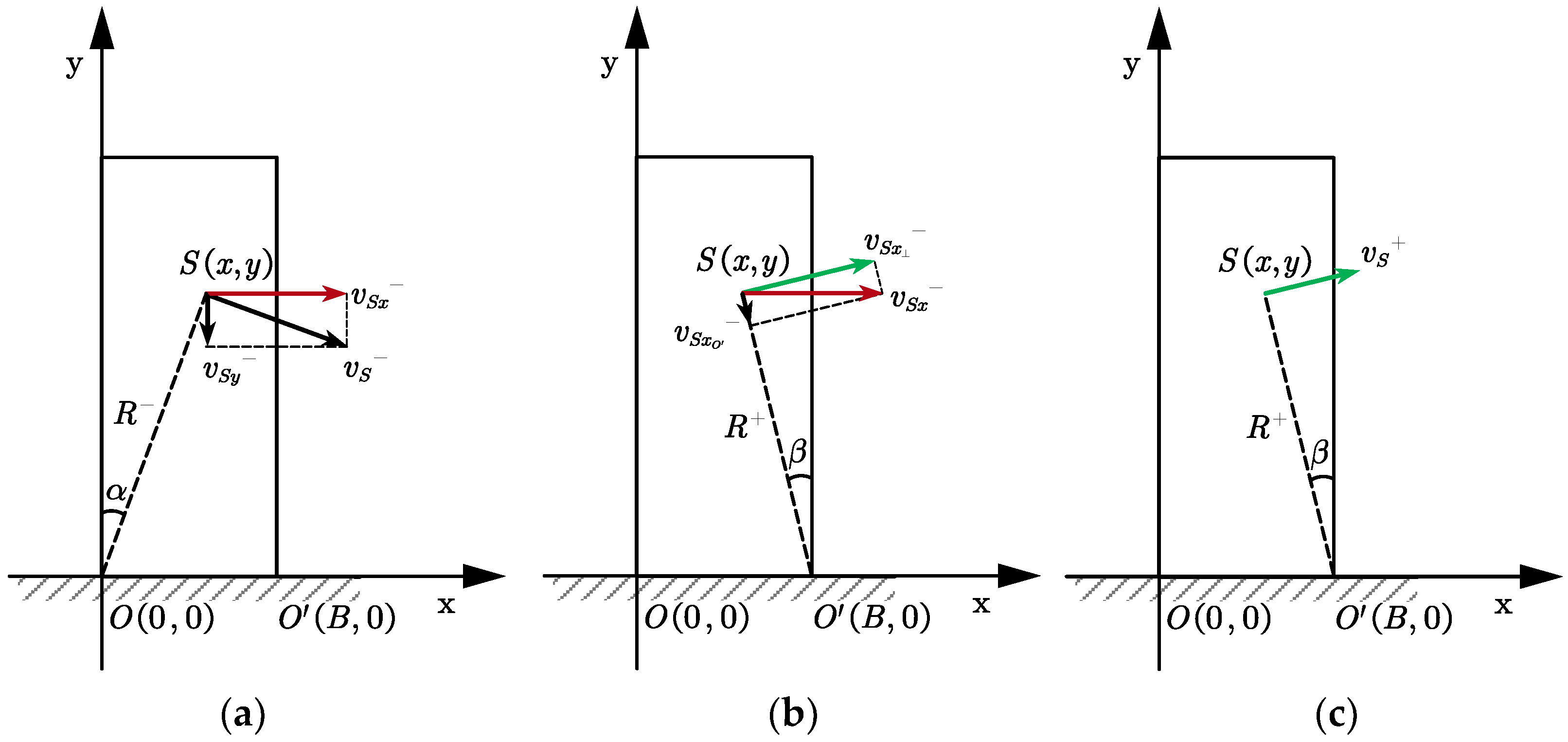
2.2. Kinetic Energy Distribution Model of the Rocking Rigid Body within the System of Mass Point

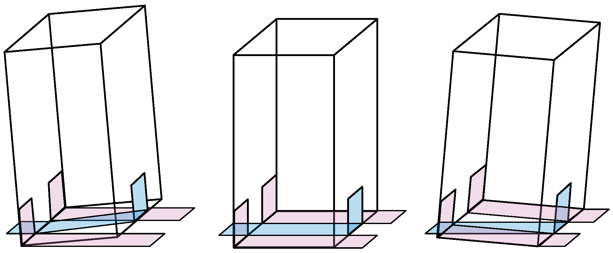
To avoid the issues encountered with the classical model of the rocking rigid body, this study establishes the kinetic energy distribution model within the system of mass points within a rocking rigid body in a Cartesian coordinate system, based on the assumptions of the classical model, as shown in Figure 2. Furthermore, the kinetic energy redistribution equation for the rocking rigid body model is derived. The variation in kinetic energy distribution of this model is divided into the following three stages.

• Moment of rotation around point $O$ before collision. The kinetic energy at point $S$ of the rigid body is decomposed into kinetic energy ${T_{Sx}}^{-}$, which is parallel to the ground, and kinetic energy ${T_{Sy}}^{-}$, which is perpendicular to the ground. Due to the collision, the kinetic energy ${T_{Sy}}^{-}$, which is perpendicular to the ground, is completely dissipated.
• Moment of collision. The kinetic energy ${T_{Sx}}^{-}$, which is parallel to the ground, is further decomposed into kinetic energy ${T_{S{x}_{O^{\prime }}}}^{-}$ along the direction $O^{\prime }S$ and kinetic energy ${T_{S{x}_{\perp }}}^{-}$ perpendicular to direction $O^{\prime }S$. The center of rotation shifts from point $O$ to point $O^{\prime }$, and the kinetic energy ${T_{S{x}_{\perp }}}^{-}$ along direction $O^{\prime }S$ is completely dissipated under the combined action of the vertical reaction force from the ground and the horizontal frictional force.
• Moment of rotation around point $O^{\prime }$ after collision. The finite element analysis conducted by Kouris et al. [25] indicates that the variation of stress within the rigid block during the collision process is quite complex, and it is not appropriate to deduce the changes in the kinetic energy distribution of the rigid body within the system of mass points based on the alteration of stresses within the rigid body. Based on the assumption that the rigid body remains undamaged during the collision, the velocity of each point within the rigid body system is redistributed under the influence of the stresses. The total sum of kinetic energy at each point of the rigid body does not increase or decrease during this process; hence, the kinetic energy ${T_{S{x}_{\perp }}}^{-}$ along the perpendicular direction $O^{\prime }S$ is redistributed into kinetic energy ${T_S}^{+}$ rotating around $O^{\prime }$.

It is clear from the kinetic energy distribution model of the particle system rocking rigid body that the first two stages are characterized by energy dissipation, where the rigid body decomposes and calculates the loss of kinetic energy at any point $S$; in contrast, during the third stage, the kinetic energy at each point of the rigid body undergoes redistribution due to internal forces. The process of kinetic energy decomposition and loss, as well as the derivation of the kinetic energy redistribution equation for this model, are described as follows.

The linear velocity of the rigid body at point $S$ immediately before the collision is

$${v_S}^{-}={\dot{\theta }}^{-}{R}^{-}$$

(6)

where $R^{-}$ represents the distance from point $S$ to point $O$.

The velocity of this point parallel to the ground is

$${v_{Sx}}^{-}={\dot{\theta }}^{-}{R}^{-}\cos \alpha$$

(7)

where $\alpha$ is the angle between $OS$ and the vertical side.

At the moment of collision, the velocity of this point perpendicular to $O^{\prime }S$ is

$${v_{S{x}_{\perp }}}^{-}={\dot{\theta }}^{-}{R}^{-}\cos \alpha \cos \beta$$

(8)

where $\beta$ is the angle between $S{O}^{\prime }$ and the vertical side.

Within the coordinate system, point $O$ serves as the origin $(0,0)$, the coordinates of point $O^{\prime }$ are $(B,0)$, and the coordinates of point $S$ are $(x,y)$; according to trigonometric relationships, Equation (8) can be rewritten as

$${v_{S{x}_{\perp }}}^{-}={\dot{\theta }}^{-}\frac{y^2}{\sqrt{y^2+{(B-x)}^2}}$$

(9)

At this time, the kinetic energy of the rigid body at point $S$ is

$${T_{S{x}_{\perp }}}^{-}=\frac{1}{2}m{\left({\dot{\theta }}^{-}\right)}^2\frac{y^4}{y^2+{(B-x)}^2}$$

(10)

where $m=\rho dxdy$ is the mass of the rigid body at point $S$.

The total kinetic energy possessed by the rigid body at this moment is

$$T^{-}=\frac{1}{2}\rho {\left({\dot{\theta }}^{-}\right)}^2{\displaystyle \underset{0}{\overset{H}{\int }}{\displaystyle \underset{0}{\overset{B}{\int }}\frac{y^4}{y^2+{(B-x)}^2}dxdy}}$$

(11)

where $T^{-}$ is the total kinetic energy before redistribution of the rigid body, $B$ is the width of the rigid body, $H$ is the height of the rigid body, and $\rho$ is the density of the rigid body.

Immediately after the collision, the kinetic energy of the rigid body is redistributed such that the velocity at any point on the rigid body conforms to the velocity of the rigid body rotating around point $O^{\prime }$. The linear velocity at point $S$ of the rigid body at this moment is

$${v_S}^{+}={\dot{\theta }}^{+}{R}^{+}$$

(12)

where $R^{+}$ is the distance from point $S$ to point $O^{\prime }$.

According to trigonometric relationships, Equation (12) can be rewritten as

$${v_S}^{+}={\dot{\theta }}^{+}\sqrt{y^2+{\left(B-x\right)}^2}$$

(13)

The kinetic energy of the rigid body at point $S$ at this time is

$${T_S}^{+}=\frac{1}{2}m{\left({\dot{\theta }}^{+}\right)}^2\left[y^2+{\left(B-x\right)}^2\right]$$

(14)

The total kinetic energy possessed by the rigid body at this time is

$$T^{+}=\frac{1}{2}\rho {\left({\dot{\theta }}^{+}\right)}^2{\displaystyle \underset{0}{\overset{H}{\int }}{\displaystyle \underset{0}{\overset{B}{\int }}\left[y^2+{\left(B-x\right)}^2\right]dxdy}}$$

(15)

The redistribution of kinetic energy alters the kinetic energy at each point of the rigid body without changing the total kinetic energy, that is, $T^{-}=T^{+}$. Thus by combining Equation (11) with Equation (15), the kinetic energy redistribution equation for the kinetic energy distribution model of the rocking rigid body within the system of mass points can be derived as

$${\left(\frac{{\dot{\theta }}^{+}}{{\dot{\theta }}^{-}}\right)}^2=\frac{{\displaystyle \underset{0}{\overset{H}{\int }}{\displaystyle \underset{0}{\overset{B}{\int }}\frac{y^4}{y^2+{(B-x)}^2}dxdy}}}{{\displaystyle \underset{0}{\overset{H}{\int }}{\displaystyle \underset{0}{\overset{B}{\int }}\left[y^2+{\left(B-x\right)}^2\right]dxdy}}}$$

(16)

Therefore, the collision restitution coefficient of the rocking rigid body kinetic energy distribution model within the system of mass points can be represented by the following equation:

$$r^2=\frac{{\displaystyle \underset{0}{\overset{H}{\int }}{\displaystyle \underset{0}{\overset{B}{\int }}\frac{y^4}{y^2+{(B-x)}^2}dxdy}}}{{\displaystyle \underset{0}{\overset{H}{\int }}{\displaystyle \underset{0}{\overset{B}{\int }}\left[y^2+{\left(B-x\right)}^2\right]dxdy}}}$$

(17)

3. Validation of the Results

To validate the rationality of the kinetic energy distribution model of the rocking rigid body within the system of mass point, this paper collects data from previous studies and derives analytical solutions for the collision restitution coefficient of both the classical model of the rocking rigid body and the kinetic energy distribution model of the rocking rigid body within the system of mass point. These are then compared with experimental values, and an error analysis is conducted.

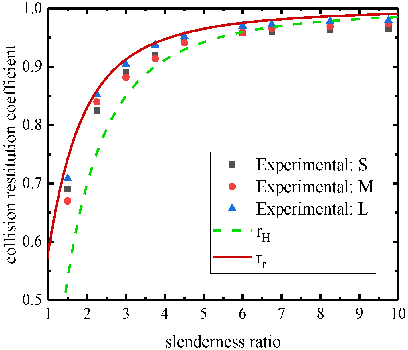
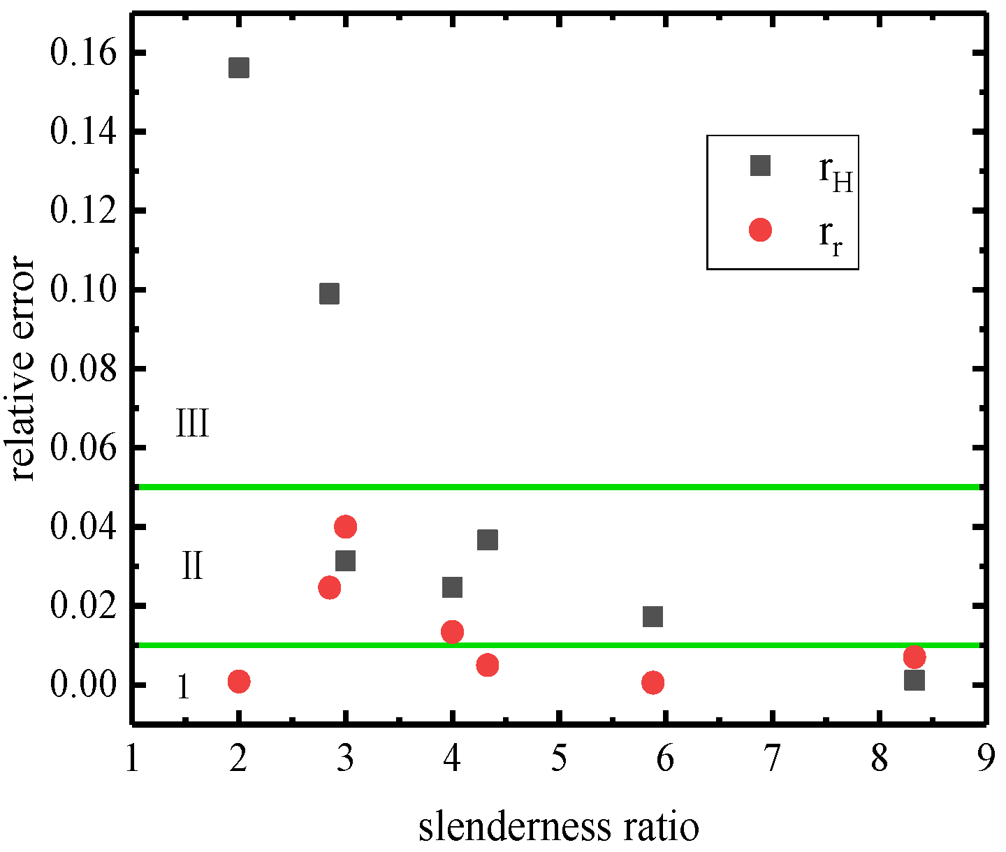
3.1. Verification of Analytical Solution under Various Slenderness Ratios

Kalliontzi et al. [30] compiled statistics on the collision restitution coefficient of the rocking rigid body and concluded that the experimental values obtained were all higher than those of the classical model of the rocking rigid body, as shown in

Table 1. Statistics on the test results of the collision restitution coefficient for rocking rigid body [30].

Slenderness Ratio (h/b)	${\mathit{r}}_{\mathit{e}}$	${\mathit{r}}_{\mathit{H}}$	Relative Error	Block and Base (Materials at Contact Interface)
2	0.787401	0.7	0.110999	wood/steel
2	0.87178	0.7	0.197045	concrete/aluminum
2.85	0.927362	0.836	0.097806	granite/granite
3	0.877496	0.85	0.033012	wood/steel
4	0.938083	0.912	0.028825	wood/steel
4	0.927362	0.912	0.017597	concrete/steel
4	0.938083	0.912	0.028825	granite/granite
4	0.948683	0.912	0.039676	wood/aluminum
4	0.921954	0.912	0.011835	steel/steel
4.33	0.959166	0.924	0.016439	steel/wood
5.88	0.974679	0.958	0.015916	granite/granite
8.33	0.979796	0.979	0	granite/granite

Note: $r_e$ represents the experimental value of the collision restitution coefficient, and $r_H$ is the collision restitution coefficient from Housner’s classical model.

.

In reality, the collision restitution coefficient measured in collision experiments varies slightly with different materials; however, since the materials used in the compiled experimental data are not prone to deformation and the collision time is extremely short, the error introduced by different materials is considered negligible. Owing to errors inherent in the testing process, for slenderness ratios that have been tested multiple times, an average value is adopted to represent the collision restitution coefficient for that specific aspect ratio.

Based on the formula for the collision restitution coefficient derived by the kinetic energy distribution model of the rocking rigid body within the system of mass point, a computation program was developed using MATLAB, as shown in Appendix A. The processed data were imported into this program to calculate the corresponding collision restitution coefficient $r_r$ for the kinetic energy distribution model of the rocking rigid body within the system of mass point, as shown in

Table 2. Comparison of collision restitution coefficients for rocking rigid body with statistical data.

Slenderness Ratio (h/b)	${\mathit{r}}_{\mathit{e}}$	${\mathit{r}}_{\mathit{H}}$	${\mathit{r}}_{\mathit{r}}$
2	0.8295905	0.7	0.83030915
2.85	0.927362	0.83666	0.90454519
3	0.877496	0.848528	0.91256288
4	0.934833	0.911043	0.94736684
4.33	0.959166	0.943398	0.95441345
5.88	0.974679	0.959166	0.97412902
8.33	0.979796	0.979796	0.98664748

Note: $r_e$ represents the experimental value of the collision restitution coefficient, $r_H$ is the collision restitution coefficient from Housner’s classical model, and $r_r$ is the collision restitution coefficient for the kinetic energy distribution model of the rocking rigid body within the system of mass point.

.

Based on the data, it is evident that the collision restitution coefficient of the kinetic energy distribution model of the rocking rigid body within the system of mass points aligns more closely with the experimental values. To visualize the relationship between the classical model of the rocking rigid body, the kinetic energy distribution model of the rocking rigid body within the system of mass points, and the experimental data, a relationship of the slenderness ratio and collision restitution coefficient was constructed, as shown in Figure 3. This figure uses the error between the collision restitution coefficient from the kinetic energy distribution model of the rocking rigid body within the system of mass points and the experimental values as the length of the error bar. The curve for the classical model of the rocking rigid body falls within the error bar range only at slenderness ratios of 3 and 8.33, whereas the error is greater than that of the kinetic energy distribution model of the rocking rigid body within the system of mass points for all other slenderness ratios.

Čeh et al. [31] conducted research on the energy dissipation of oscillating aluminum blocks using three sets (S—small, M—medium, L—large) of blocks. Each set contained 10 aluminum blocks with different slenderness ratios. To prevent slipping and bouncing, tape was applied between the block and the base, as shown in Figure 4.

Using the computational program developed in MATLAB, the collision restitution coefficient $r_H$ for the classical model of the rocking rigid body and the collision restitution coefficient $r_r$ for the kinetic energy distribution model of the rocking rigid body within the system of mass points were calculated based on the experimental data. The specimen parameters, experimental data, and calculation results are presented in

Table 3. The experimental results for the collision restitution coefficient of the rocking rigid body by Čeh et al. [31].

Block	m (g)	Slenderness Ratio (h/b)	re	rH	rr
S1	113.3	1.5	0.69	0.538	0.743
S2	161.2	2.25	0.825	0.753	0.859
S3	226.6	3	0.89	0.850	0.913
S4	274.5	3.75	0.919	0.900	0.941
S5	339.6	4.5	0.948	0.929	0.958
S6	453.2	6	0.958	0.959	0.975
S7	500.8	6.75	0.96	0.968	0.980
S8	614.1	8.25	0.964	0.978	0.986
S9	727.4	9.75	0.966	0.984	0.990
M1	363.6	1.5	0.67	0.538	0.743
M2	544.4	2.25	0.84	0.753	0.859
M3	727.2	3	0.882	0.850	0.913
M4	907.7	3.75	0.914	0.900	0.941
M5	1089.6	4.5	0.941	0.929	0.958
M6	1453.2	6	0.959	0.959	0.975
M7	1634	6.75	0.966	0.968	0.980
M8	1997.6	8.25	0.969	0.978	0.986
M9	2361.2	9.75	0.974	0.984	0.990
L1	856.6	1.5	0.708	0.538	0.743
L2	1284.3	2.25	0.852	0.753	0.859
L3	1713.2	3	0.904	0.850	0.913
L4	2140.9	3.75	0.937	0.900	0.941
L5	2569.2	4.5	0.952	0.929	0.958
L6	3425.8	6	0.97	0.959	0.975
L7	3853.5	6.75	0.972	0.968	0.980
L8	4710.1	8.25	0.978	0.978	0.986
L9	5566.7	9.75	0.979	0.984	0.990

Note: $r_e$ represents the experimental value of the collision restitution coefficient, $r_H$ is the collision restitution coefficient from Housner’s classical model, and $r_r$ is the collision restitution coefficient for the kinetic energy distribution model of the rocking rigid body within the system of mass point.

.

Similarly, Table 3 shows that the collision restitution coefficient derived from the kinetic energy distribution model of the rocking rigid body within the system of mass points is in better agreement with the experimental values. To more clearly visualize the relationship between the classical model of the rocking rigid body, the kinetic energy distribution model of the rocking rigid body within the system of mass points, and the experimental data, a relationship between the slenderness ratio and collision restitution coefficient was created, as depicted in Figure 5.

Figure 5 clearly demonstrates that the collision restitution coefficient for the aluminum blocks in Group L is closer to the theoretical values predicted by the kinetic energy distribution model of the rocking rigid body within the system of mass points. Additionally, the experimental data shows a relatively stable deviation from the theoretical predictions of the kinetic energy distribution model of the rocking rigid body within the system of mass point. The deviation between the experimental data and the classical model of the rocking rigid body increases gradually as the aspect ratio decreases.

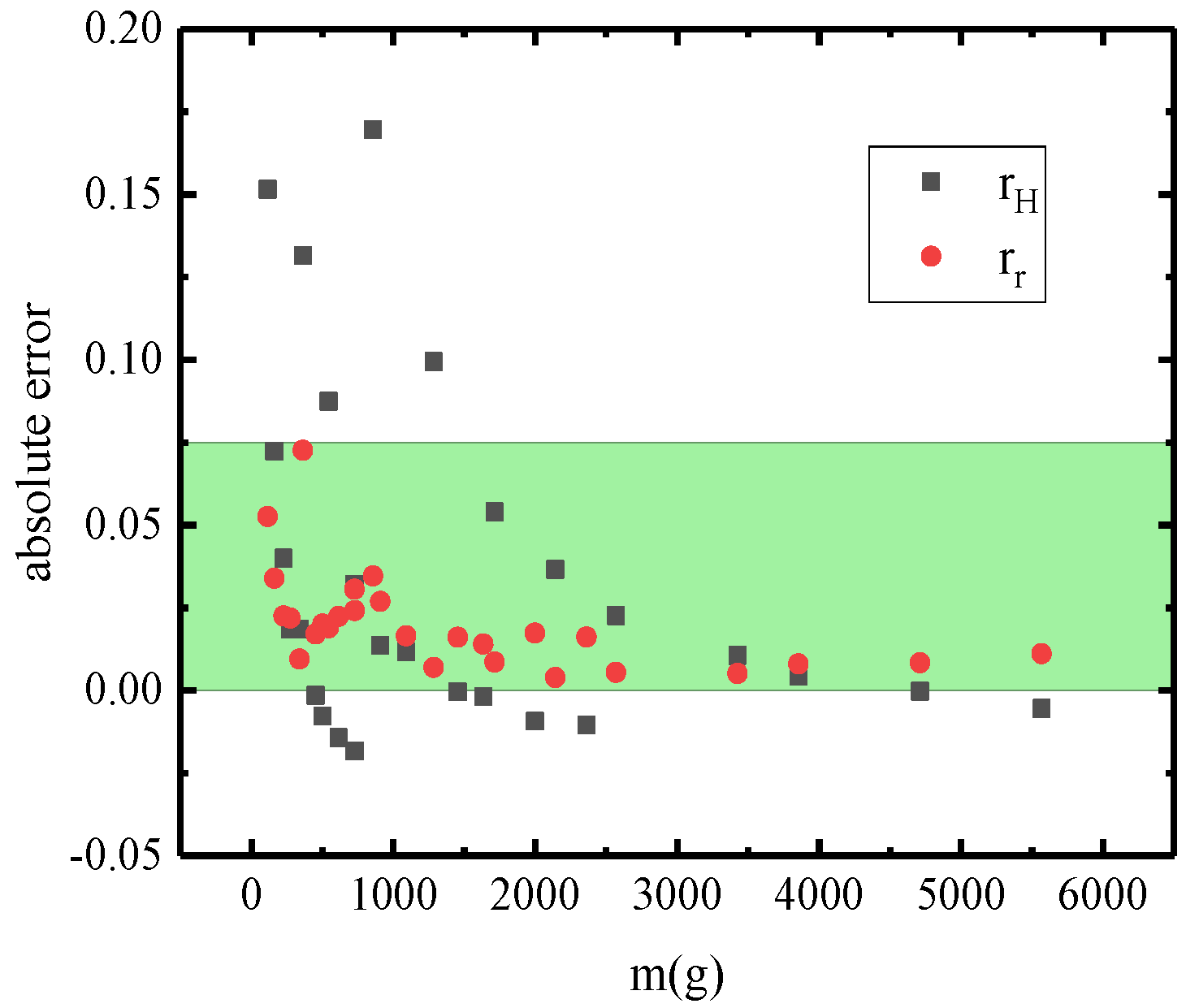
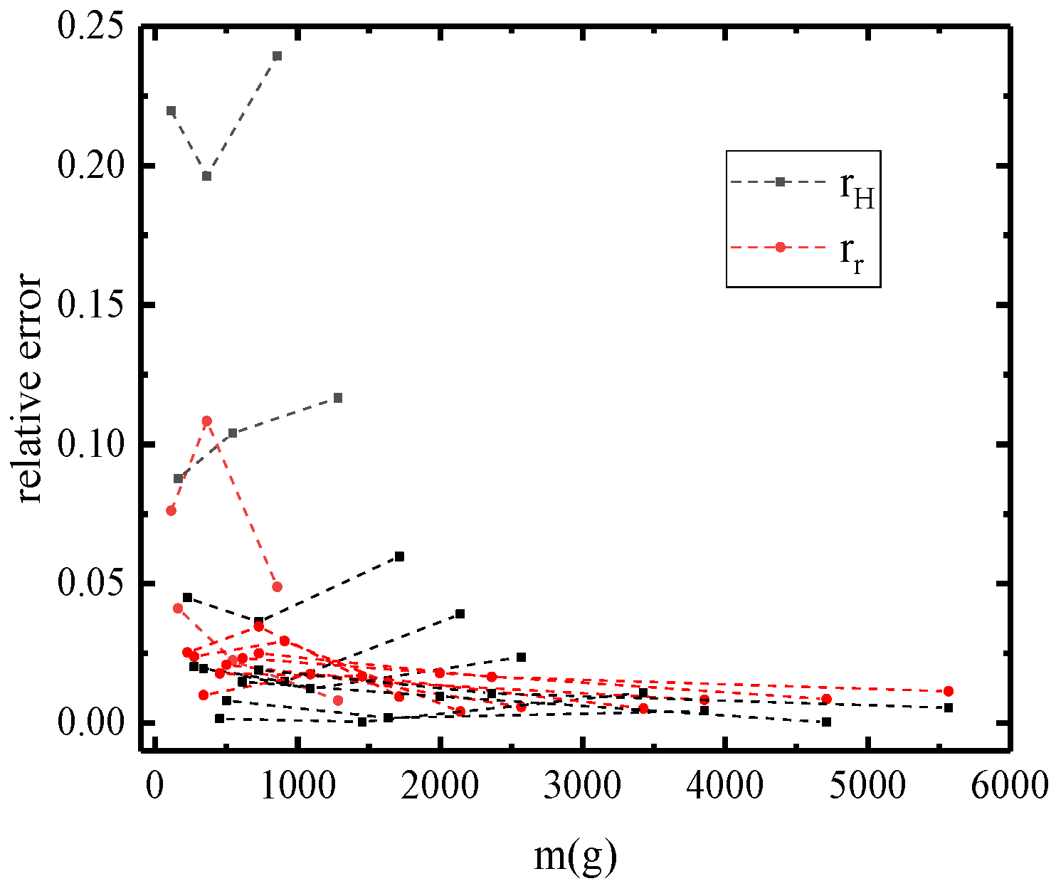
3.2. Correlation and Error Analysis

Analysis reveals a correlation coefficient of 0.946 between the theoretical values of the kinetic energy distribution model of the rocking rigid body within the system of mass points and the statistical data. The correlation coefficients with the experimental values for Groups S, M, and L are 0.998, 0.996, and 0.998, respectively. To facilitate further analysis, scatter plots depicting the relative errors between the theoretical values of the two models and the four data sets are provided in Figure 6 and Figure 7.

In the figures, the relative errors are divided into three zones. Zone I represents errors less than 1%, Zone II represents errors greater than 1% but less than 5%, and Zone III represents errors greater than 5%. As can be seen from Figure 6, the relative errors for the classical model of the rocking rigid body are primarily distributed in Zones II and III, while the relative errors for the kinetic energy distribution model of the rocking rigid body within the system of mass points are all within Zones I and II.

Figure 7 reveals that for the three sets of data, when the slenderness ratio is less than 6, the theoretical values from the kinetic energy distribution model of the rocking rigid body within the system of mass points are more consistent with the experimental data. For Groups S and M, the advantage of the kinetic energy distribution model of the rocking rigid body within the system of mass points over the classical model of the rocking rigid body is not significant, but for Group L, the superiority of the kinetic energy distribution model of the rocking rigid body within the system of mass points is more pronounced. Furthermore, the figure illustrates that the error associated with the kinetic energy distribution model of the rocking rigid body under the system of mass points remains largely constrained within 10% across the three test groups. Only one exception occurred in the Group M experiment. The analysis shows that it is easier to produce errors in smaller components because the experiment is in a non-ideal state. Consequently, it is necessary to further analyze the influence of quality.

The experiments were not conducted under ideal conditions: collisions were not instantaneous, and some horizontal kinetic energy was consumed due to friction, with additional energy loss attributed to the tape affixed to the bottom of the blocks. To facilitate analysis, a scatter plot of the absolute error between theoretical and experimental values was created using the mass of the blocks as the independent variable (since the experiments fall between two theoretical values, for ease of comparison, the absolute error for $r_r$ is represented by $r_r-r_e$, and the absolute error for $r_H$ is represented by $r_e-r_H$), as shown in Figure 8. The relative errors between the theoretical values and experimental data for the same slenderness ratio are plotted on the same line chart, as depicted in Figure 9.

Figure 8 indicates that the absolute errors of the kinetic energy distribution model of the rocking rigid body within the system of mass points decrease gradually with an increase in mass and, unlike the classical model of the rocking rigid body, exhibit a relatively stable absolute error.

Figure 9 shows that at the same slenderness ratio, the relative errors of the kinetic energy distribution model of the rocking rigid body within the system of mass points tend to decrease with an increase in mass, whereas the relative error for the classical model of the rocking rigid body increases as the mass increases.

Based on the above analysis, it can be seen that the model proposed in this paper has a strong correlation with the test data, and the correlation coefficient is greater than 0.9. The error is more stable than the classical model, and the relative errors are basically controlled within 5%. In addition, since the larger the mass of the component is, the less affected by the environment, the model shows a stronger adaptability to large components (smaller error), indicating that the model can be applied to components with larger mass in engineering. Further research is needed to make it also applicable to components with smaller mass.

4. Conclusions

To refine the model of the rocking rigid body, this study proposes a phasic energy dissipation and kinetic energy redistribution model for the rocking rigid body within the system of mass points. This research conducts a step-by-step analysis of the collision process within the model and redistributes the kinetic energy post-collision, deriving an analytic solution for the collision restitution coefficient under this model. By analyzing the correlation coefficients and relative errors between the collision restitution coefficient from the proposed model and the classical model of the rocking rigid body against experimental data, the results indicate that the proposed model outperforms the classical model of the rocking rigid body. This confirms the validity of the presented model, demonstrating that the numerical solutions are accurate and reliable, leading to the following conclusions and recommendations.

• The kinetic energy distribution model of the rocking rigid body within the system of mass points, starting from the kinetic energy and based on the energy dissipation mechanism during collisions, calculates the energy loss and conservation phases separately, which aligns more closely with reality and shows a higher degree of agreement with experimental data. Since small components initially have lower kinetic energy and are subject to more influencing factors, the advantages of this theory are more prominent in larger structures.
• The analytic solution presented in this study is derived under the ideal conditions of extremely short collision times and negligible horizontal kinetic energy loss. However, actual collisions involve a brief contact time, primarily related to the materials involved in the collision and the instantaneous velocity. Therefore, the precision of the corresponding solutions varies with different materials and masses of the rigid bodies. If the collision time could be determined and the loss of horizontal kinetic energy taken into account, the accuracy of the solutions could be further improved.
• In order to further improve the proposed model to explore the energy loss caused by non-instantaneous collision and friction in the swaying rigid body, it is necessary to analyze the contact between the rigid body and the ground during the collision process. The collision surface of the rigid body can be divided into a certain number of points. By introducing parameters such as the mass and elastic modulus of the rigid body, the force at each point in the collision process and the contact time with the ground can be calculated, and the kinetic energy lost during the collision process can be calculated more accurately.
• The rigid bodies in the kinetic energy distribution model of the rocking rigid body within the system of mass points are established as homogeneous regular rectangular blocks in a two-dimensional plane. To better align with practical engineering applications, research into the collision restitution coefficient for three-dimensional-space rocking rigid bodies is necessary. This model provides new insights for the analysis of rocking in non-homogeneous and irregularly shaped rigid bodies. Further research can be conducted on non-homogeneous or irregularly shaped rigid bodies to refine the existing model of the rocking rigid body.
• In order to expand the proposed model, the idea of finite element analysis can be incorporated into subsequent research, and the rigid body can be divided into multiple units to calculate its kinetic energy loss and conversion, so as to analyze the collision of non-homogeneous and irregular rigid bodies in three-dimensional space, making its application more practical.

References

1. Jeong, M.Y.; Lee, H.; Kim, J.H.; Yang, I.Y. Chaotic behavior on rocking vibration of rigid body block structure under two―dimensional sinusoidal excitation (in the case of no sliding). KSME Int. J. 2003, 17, 1249–1260. [Google Scholar] [CrossRef]
2. Jeong, M.Y.; Yang, I.Y. Characterization on the rocking vibration of rigid blocks under horizontal harmonic excitations. Int. J. Precis. Eng. Manuf. 2012, 13, 229–236. [Google Scholar] [CrossRef]
3. Zheng, X.W.; Li, H.N.; Gardoni, P. Hybrid Bayesian-Copula-based risk assessment for tall buildings subject to wind loads considering various uncertainties. Reliab. Eng. Syst. Saf. 2023, 233, 109100. [Google Scholar] [CrossRef]
4. Zheng, X.W.; Li, H.N.; Shi, Z.Q. Hybrid AI-Bayesian-based demand models and fragility estimates for tall buildings against multi-hazard of earthquakes and winds. Thin-Walled Struct. 2023, 187, 110749. [Google Scholar] [CrossRef]
5. Housner, G.W. The behavior of inverted pendulum structures during earthquakes. Bull. Seismol. Soc. Am. 1963, 53, 403–417. [Google Scholar] [CrossRef]
6. Zhao, Z.; Su, X. Literature review of researches on rigid body model of rocking structure. Eng. Mech. 2019, 36, 12–24. [Google Scholar]
7. Jia, C.; Pan, J.; Li, J.; Jia, C.; Pan, J.; Li, J.; Ma, L. Seismic analysis of eccentric single-rigid-body considering the influence of colliding-to-wall. J. Vib. Shock. 2022, 41, 116–123. [Google Scholar]
8. Beck, J.L.; Skinner, R.I. The seismic response of a reinforced concrete bridge pier designed to step. Earthq. Eng. Struct. Dynamics 1973, 2, 343–358. [Google Scholar] [CrossRef]
9. Du, X.-L.; Zhou, Y.-L.; Han, Q.; Wang, Z. State-of-the-art on rocking piers. Earthq. Eng. Eng. Dyn. 2018, 38, 1–11. Available online: https://dzgc.paperonce.org/#/digest?ArticleID=2426 (accessed on 27 December 2023).
10. Hukelbridge, A.A.; Clough, R.W. Preliminary Experimental Study of Seismic Uplift of a Steel Frame; Report No. UCB/EERC-77/22; University of California: Berkely, CA, USA, 1977. [Google Scholar]
11. Hukelbridge, A.A. Earthquake Simulation Tests of a Nine Story Steel Frame with Columns Allowed to Uplift; Report No. UCB/EERC-77/23; University of California: Berkely, CA, USA, 1977. [Google Scholar]
12. Zhou, Y.; Lü, X. State-of-the-art on rocking and self-centering structures. J. Build. Struct. 2011, 32, 1–10. [Google Scholar]
13. Yim, C.; Chopra, A.K.; Joseph, P. Rocking response of rigid blocks to earthquake. Earthq. Eng. Struct. Dyn. 1980, 8, 565–587. [Google Scholar] [CrossRef]
14. Aslam, M.; Scalise, D.T.; Godden, W.G. Earthquake rocking response of rigid bodies. J. Struct. Div. 1980, 106, 377–392. [Google Scholar] [CrossRef]
15. Cormack, L.G. The design and construction of the major bridges on the mangaweka rail deviation. Trans. Inst. Prof. Eng. New Zealand 1988, 15, 16–23. [Google Scholar]
16. Apostolou, M.; Gazetas, G.; Garini, E. Seismic response of slender rigid structures with foundation uplifting. Soil Dyn. Earthq. Eng. 2007, 27, 642–654. [Google Scholar] [CrossRef]
17. Marriott, D.; Pampanin, S.; Palermo, A. Quasi-static and pseudo-dynamic testing of unbonded post-tensioned rocking bridge piers with external replaceable dissipaters. Earthq. Eng. Struct. Dyn. 2009, 38, 331–354. [Google Scholar] [CrossRef]
18. Guo, T.; Cao, Z.; Xu, Z.; Lu, S. Cyclic load tests on self-centering concrete pier with external dissipators and enhanced durability [J]. J. Struct. Eng. 2015, 142, 04015088. [Google Scholar] [CrossRef]
19. Han, Q.; Jia, Z.L.; Xu, K.; Zhou, Y.; Du, X. Hysteretic behavior investigation of self-centering double-column rocking piers for seismic resilience. Eng. Struct. 2019, 188, 218–232. [Google Scholar] [CrossRef]
20. Han, Q.; Jia, Z.; He, W.; Xiao, Y.; Jia, J.; Du, X. Seismic design method and its engineering application of self-centering double-column rocking bridge. China J. Highw. Transp. 2017, 30, 169–177. [Google Scholar]
21. Mashal, M.; Palermo, A. Low-damage seismic design for accelerated bridge construction. J. Bridge Eng. 2019, 24, 04019066. [Google Scholar] [CrossRef]
22. Zhou, Y.; Zhang, J.; Han, Q.; Zhou, Y.; Zhang, J.; Han, Q.; Cheng, S.; He, H. Effect of viscous dampers on seismic response of rocking double-column bents under near-field ground motions with strong pulses. China Civ. Eng. J. 2020, 53, 288–293. [Google Scholar]
23. Kalliontzis, D.; Schultz, A.E.; Sritharan, S. Generalized dynamic analysis of structural single rocking walls (SRWs). Earthq. Eng. Struct. Dyn. 2020, 49, 633–656. [Google Scholar] [CrossRef]
24. Avgenakis, E.; Psycharis, I. An integrated macroelement formulation for the dynamic response of inelastic deformable rocking bodies. Earthq. Eng. Struct. Dyn. 2020, 49, 1072–1094. [Google Scholar] [CrossRef]
25. Kouris, E.-G.S.; Kouris, L.-A.S.; Konstantinidis, A.A.; Kourkoulis, S.K.; Karayannis, C.G.; Aifantis, E.C. Stochastic dynamic analysis of cultural heritage towers up to collapse. Buildings 2021, 11, 296. [Google Scholar] [CrossRef]
26. Kazantzi, A.K.; Lachanas, C.G.; Vamvatsikos, D. Seismic response distribution expressions for on-ground rigid rocking blocks under ordinary ground motions. Earthq. Eng. Struct. Dyn. 2021, 50, 3311–3331. [Google Scholar] [CrossRef]
27. Várkonyi, P.L.; Kocsis, M.; Ther, T. Rigid impacts of three-dimensional rocking structures. Nonlinear Dyn. 2022, 107, 1839–1858. [Google Scholar] [CrossRef]
28. Thomaidis, I.M.; Camara, A.; Kappos, A.J. Dynamics and seismic performance of asymmetric rocking bridges. J. Eng. Mech. 2022, 148, 04022003. [Google Scholar] [CrossRef]
29. Schau, H.; Johannes, M. Rocking and sliding of unanchored bodies subjected to seismic load according to conventional and nuclear rules. In Proceedings of the 4th International Conference on Computational Methods in Structural Dynamics and Earthquake Engineering, Kos Island, Greece, 12–14 June 2013. [Google Scholar]
30. Kalliontzis, D.; Sritharan, S.; Schultz, A. Improved coefficient of restitution estimation for free rocking members. J. Struct. Eng. 2016, 142, 06016002. [Google Scholar] [CrossRef]
31. Čeh, N.; Jelenić, G.; Bićanić, N. Analysis of restitution in rocking of single rigid blocks. Acta Mech. 2018, 229, 4623–4642. [Google Scholar] [CrossRef]
32. Anagnostopoulos, S.; Norman, J.; Mylonakis, G. Fractal-like overturning maps for stacked rocking blocks with numerical and experimental validation. Soil Dyn. Earthq. Eng. 2019, 125, 105659. [Google Scholar] [CrossRef]
Figure 1. Classical model of the rocking rigid body [5].
Buildings 14 02119 g001
Figure 2. The kinetic energy distribution model of the rocking rigid body within the system of mass point: (a) moment before collision; (b) moment of collision; and (c) moment after collision.
Buildings 14 02119 g002
Figure 3. Slenderness ratio versus collision restitution coefficient curves for statistical data.
Buildings 14 02119 g003
Figure 4. Rigid body-tape systems to avoid slipping and bouncing [31].
Buildings 14 02119 g004
Figure 5. Slenderness ratio versus collision restitution coefficient relationships for the three sets of data.
Buildings 14 02119 g005
Figure 6. Relative errors between the theoretical and statistical data.
Buildings 14 02119 g006
Figure 7. Relative errors between the theoretical values and the experimental data measured by Čeh [31]: (a) the errors between the theoretical values and the data from Group S; (b) the errors between the theoretical values and the data from Group M; (c) the errors between the theoretical values and the data from Group L.
Buildings 14 02119 g007
Figure 8. Absolute errors between the theoretical values and experimental data measured by Čeh [31].
Buildings 14 02119 g008
Figure 9. Relative errors between the theoretical and experimental data for the same slenderness ratio.
Buildings 14 02119 g009