There was an error in the derivation of the non-classical boundary conditions presented in the original publication [1]. Specifically, the strain was assumed positive in the -direction, at both ends of the bar and , following the formulation of the classical elasticity. However, this assumption was incorrect. A detailed analytical derivation of the boundary conditions revealed that the strain is positive in the -direction only at and negative at . The following corrections have been implemented:
- Text Correction 1
Five new paragraphs detailing the analytical derivation of the boundary conditions have been added to the end of Section 2:
Furthermore, the stress resultants—namely, the axial force and the double axial force —are given by [6]:
It is important to note that the double axial force arises due to the material’s microstructure and vanishes when . In this case, the stress resultants also reduce to the classical forms.
The relevant boundary conditions—both classical and non-classical—can be derived from the general three-dimensional gradient elasticity theory [19]. These are expressed in vector notation and can be categorized as either essential or natural boundary conditions:
where is the displacement vector, denotes the external surface tractions, is the strain vector, is a third-order tensor representing double forces per unit area, and is the outward normal vector to the surface of the body.
For the specific one-dimensional problem considered here, the classical boundary conditions are imposed at the ends of the bar and . At these ends, either the axial displacement or the axial force is prescribed:
where is the unit vector in the -direction.
Additionally, the non-classical boundary conditions can be specified at the bar ends, where either the strain or the double axial force is prescribed:
It is important to emphasize the sign conventions used: the displacement , axial force , and double axial force are considered positive when directed along the positive -axis at both ends. In contrast, the strain is positive in the -direction only at and negative at .
Accordingly, the complete set of classical and non-classical boundary conditions applicable to this problem at the bar ends and can be stated as follows:
- Text Correction 2
The relevant boundary conditions required for the derivation of the shape functions have been incorporated in Section 3.1, Paragraph 3:
( for , for , for , and for )
- Text Correction 3
In the original publication, there was a mistake in the expression of the second shape function . A correction has been made in Section 3.1, Equation (13):
- Error in Figure
In the original publication, there was a mistake in Figure 4 in the depiction of the second shape function. The corrected Figure 4 appears below.
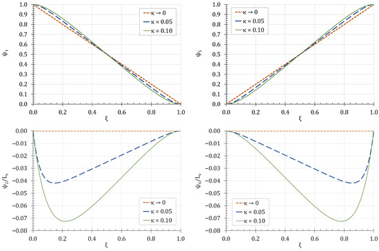
Figure 4.
Shape functions of the gradient truss element.
- Text Correction 4
In the original publication, the mistake in the expression of the second shape function affected the formulation of the exact stiffness matrix for the gradient truss element in local coordinates. This has been corrected in Section 3.1, Equation (19):
where is the ratio of the microstructural length, , over the element’s length, .
- Text Correction 5
In the original publication, the mistake in the expression of the second shape function affected the exact mass matrix of the gradient truss element in local coordinates. The corrected values for the elements , , and are provided in Section 3.1, Equations (33), (37) and (38):
- Text Correction 6
The following sentence has been added to the end of Section 3.2:
Note that, for brevity, the previous relations use the notation .
- Text Correction 7
The displacement percentage reductions have been revised based on the updated results in the second example. A correction has been made in Section 4.2, Paragraph 1:
Specifically, exhibits a reduction of 30.58% relative to the CE solution when , while the corresponding reductions of and are 20.55% and 20.63%, respectively.
- Text Correction 8
The percentage increase in the natural frequencies has been updated based on the revised results from the second example. A correction has been made in Section 4.2, Paragraph 2:
For example, when , and show an approximate 12% increase relative to the CE solution. In contrast, increases by 16.35%, while displays a modest increase of 5.21%.
- Error in Table
The displacement and strains of the gradient truss of the second example have been updated based on the latest results. The corrected Table 5 appears below.

Table 5.
Displacements (m) and strains (rad) at various DoF of the gradient truss of Example 4.2 for various values of the microstructural length (m).
The first four natural frequencies of the gradient truss of the second example have been updated based on the latest results. The corrected Table 6 appears below.
Table 6.
First four natural frequencies ( of the gradient truss of Example 4.2 for various values of the microstructural length .
The first four natural frequencies of the gradient truss of the second example for have been updated based on the latest results. The corrected Table 7 appears below.
Table 7.
First four natural frequencies ( of the gradient truss of Example 4.2 for .
The first four natural frequencies of the gradient truss of the second example for have been updated based on the latest results. The corrected Table 8 appears below.
Table 8.
First four natural frequencies ( of the gradient truss of Example 4.2 for .
- Reference
A new reference “Polyzos, D.; Tsepoura, K.G.; Tsinopoulos, S.V.; Beskos, D.E. A Boundary Element Method for Solving 2-D and 3-D Static Gradient Elastic Problems: Part I: Integral Formulation. Comput. Methods Appl. Mech. Eng. 2003, 192, 2845–2873. https://doi.org/10.1016/S0045-7825(03)00289-5” has been added to the original reference list as [19]. With this correction, the order of some references has been adjusted accordingly.
The authors state that the scientific conclusions are unaffected. This correction was approved by the Academic Editor. The original publication has also been updated.
Reference
- Tsiatas, G.C.; Charalampakis, A.E.; Giannakopoulos, A.E.; Tsopelas, P. Static and Dynamic Analysis of Strain Gradient Planar Trusses. Buildings 2024, 14, 4031. [Google Scholar] [CrossRef]

Disclaimer/Publisher’s Note: The statements, opinions and data contained in all publications are solely those of the individual author(s) and contributor(s) and not of MDPI and/or the editor(s). MDPI and/or the editor(s) disclaim responsibility for any injury to people or property resulting from any ideas, methods, instructions or products referred to in the content. |
© 2025 by the authors. Licensee MDPI, Basel, Switzerland. This article is an open access article distributed under the terms and conditions of the Creative Commons Attribution (CC BY) license (https://creativecommons.org/licenses/by/4.0/).