Abstract
In this work, we generated a set of random representative volume elements (RVEs) of unidirectional composites considering actual noncircular cross-sections and positions of fibers with the aid of a shape-library approach. The cross-section of the noncircular carbon fiber was extracted from the M55J/M18 composite using image processing and a signed-distance-based mesh trimming scheme, and they were stored in a particle-shape library. The obtained noncircular fibers randomly chosen from the particle-shape library were applied to random fiber array generation algorithms to generate RVEs of various fiber volume fractions. To check the randomness of the proposed RVEs, we calculated spatial and physical metrics, and concluded that the proposed method is sufficiently random. Furthermore, to compare the effective elastic properties and the maximum von Mises stress in the matrix, it was applied to composite materials with different relative ratios of elastic moduli of M55J/M18 and T300/PR319. In the case of T300/PR319 having a high (relative ratio of the transverse elastic moduli), simulation results were deviated up to about 5% in the effective elastic properties and 13% in the maximum von Mises stress in the matrix according to the fiber shapes.
1. Introduction
Random fiber generators can provide arbitrary arrangements of fibers or fillers in a two-dimensional (2D) or three-dimensional (3D) space, which approximate the shape of the microstructure of a composite material. As a result, the representative volume elements (RVEs) simulating the real microstructure can be constructed; they have been commonly used in studying the mechanical behavior of composite materials and structures. RVEs can be an excellent micromechanical-based model that predicts equivalent physical properties, such as the strength, stiffness, coefficient of thermal expansion, and so forth of composites. However, for efficient modeling of these RVE models, there are some situations in which the shape of the fiber/filler is excessively simplified into a circle, sphere, cylinder, or disc. Sometimes, these approximations could distort the effect of stress concentration between fibers, resulting in less accurate prediction of the equivalent stiffness and strength. In addition, the actual fiber has a more complex shape due to various manufacturing defects such as waviness [1,2], misalignment [3,4], crater, and so forth [5,6,7]. In particular, in the case of unidirectional composites, unlike the cross-sections of glass fibers, which are almost circular, those of carbon fibers have been reported to have various shapes, such as circular, triangular, C-shaped, kidney-shaped, and so forth, so that the stress concentration between the fibers is complicated [8,9,10,11,12,13,14,15,16]. Moreover, it has a larger specific surface area due to its irregular shape; therefore, better mechanical properties are attained [17]. It has also been found that it is not appropriate to simplify circular fibers using the popular Hough transform when having irregular fiber shapes [18].
To construct more actual RVEs, various fiber shapes were proposed to see the effect of the shape of fibers for the mechanical properties. However, their shape was still regular because it was derived from the mathematical equation, not real experimental data [13,14]. Thus, an algorithm based on the shape from the experimental data is urgently required to generate realistic RVEs. Recently, a shape-library approach was introduced to generate the carbon nanotube morphology from a database constructed from the experimental data through micro-computed tomography (CT) analyses to predict the electrical resistivity [19], and it turned out that a prediction with the shape-library approach was accurate as well as promising because it can reflect the experimental data into a prediction model. Similarly, 3D particle shapes were extracted from CT analysis; they were used to reconstruct many RVE samples [20,21]. However, no studies have been reported on the generation of RVEs using a shape library composed of 2D particle shapes of unidirectional composites.
The objective of this work is to generate RVEs considering the actual fiber shape of unidirectional composites with the aid of a shape-library approach. A particle-shape library was constructed by extracting fiber shapes from real microscopic images of M55J/M18 composites whose fiber shape is rather irregular using the signed-distance-based mesh trimming scheme, which we proposed in our previous work [18,22]. Then, random sequential expansion (RSE) [23] and random fiber removal (RFR) [24,25] algorithms were applied to generate many RVE samples with various volume fractions (). The spatial and physical statistical metrics were calculated to confirm the randomness of the actual noncircular fiber arrangements. In addition, to compare the performance of the proposed RVEs with that of conventional RVEs with circular fibers, the effective elastic properties were compared by applying the properties of M55J/M18 and T300/PR319 composites, which are unidirectional composites showing transverse isotropy. Finally, the trend of the maximum von Mises stress in the matrix was investigated to determine the effect of shapes of fibers on the fracture strength of the material. To the best of our knowledge, predicting the mechanical properties considering complex actual fiber shapes by a shape-library approach has never been attempted yet despite its importance in the society of the composites.
The remaining sections of this paper are organized as follows. Section 2 explains how finite element (FE) meshes are constructed with actual fibers from microscope images. Furthermore, a brief description and a modification of the RSE and RFR algorithms for actual fibers are presented. Next, in Section 3, we use spatial and physical statistical metrics to demonstrate the performance of the proposed scheme for randomness and the prediction of elastic modulus, and we investigate the maximum stress concentration patterns of the matrix according to fiber shapes and . Finally, Section 4 closes this paper with concluding remarks.
2. Random RVE Generation Using Actual Noncircular Fibers from the Particle-Shape Library
2.1. The Particle-Shape Library Construction of Actual Noncircular Fibers Using a Microscopic Image of the M55J/M18 Composite
According to our previous work, a FE model was generated from a microscopic image of the M55J/M18 composite [18] by the level set method and the trimming mesh method [22]. First, we binarized the microscopic image (see Figure 1a,b) by a black-white filter and proper noise removal, and then used it to generate a voxel mesh after resizing the image whenever necessary (see Figure 1c). The minimum signed distance function (SDF) of the image was obtained using the level set method (see Figure 1d), and the trimmed mesh technique was applied to smooth the voxel mesh (see Figure 1e). Finally, remeshing was conducted to reconstruct the four-noded quadrilateral elements (see Figure 1f).
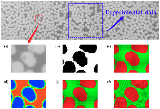
Figure 1.
Procedure of generating FE model from a microscopic image of M55J/M18 composite: (a) original image, (b) binary image, (c) voxel mesh with image rescaling, (d) minimum SDF, (e) trimmed mesh, and (f) remeshing to quadrilateral elements.
From the final FE model, a set of the outer nodes of the intact fibers was stored in the particle-shape library of fibers as shown in Figure 2. In this work, we stored 482 fiber samples in the particle-shape library. Furthermore, it can be seen that the actual fibers of the M55J/M18 composite are concave and convex.
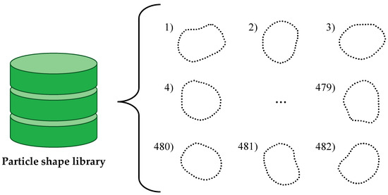
Figure 2.
Schematic illustration of the particle-shape library consisting of actual noncircular fibers.
2.2. RVE Generation with Diverse
Many RVE samples were generated with various values of 60%, 55%, 45%, 35%, 25%, 15%, and 5% by randomly choosing the geometry of actual fibers from the particle-shape library created as described in the previous subsection. To arrange the fibers properly in a square domain, the RSE and RFR algorithms were employed with proper modification as described in the following subsection.
2.2.1. RVE Generation Using the RSE Algorithm
The procedure for applying the RSE algorithm [23] and its modification is introduced as follows (see Figure 3). An arbitrary rotation procedure of fibers is added to the beginning of the original RSE algorithm. A flowchart of the algorithm is shown in Figure 4.
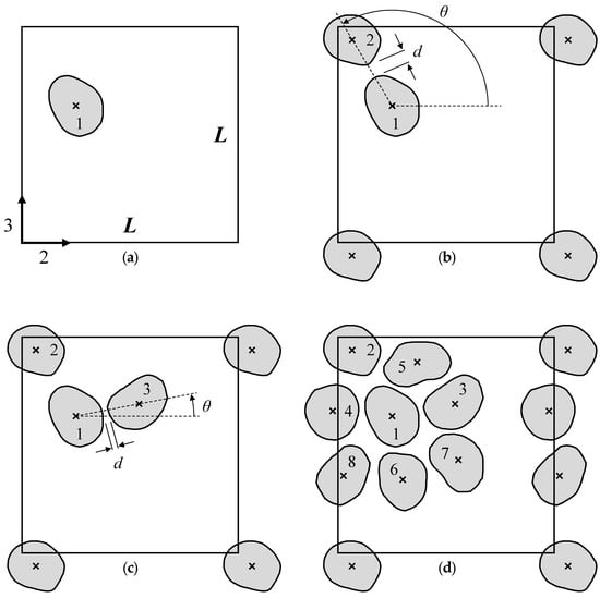
Figure 3.
Schematic illustration of the RSE algorithm with actual fibers: (a) step 2, (b) step 3, and (c,d) step 4.
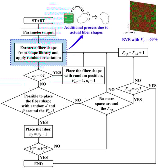
Figure 4.
Flowchart of the RSE algorithm and its modification for the actual noncircular fibers.
- After a fiber shape is randomly chosen from the particle-shape library, it is rotated at arbitrary angles around its centroid to give a random orientation to the fiber. Here, denotes the current number of fibers used in RVE.
- For the first fiber ( = 1), it is placed in any position in the square window of (see Figure 3a). The first fiber is set as the reference fiber ().
- Then, step 1 is repeated to choose the new fiber to be placed from the particle-shape library. The new fiber is placed to satisfy the random minimum distance and random orientation angle between the new fiber and . Additionally, it is necessary to ensure that the minimum distance between the new fiber and the existing fibers is at least . The values and can be determined according to the requested fiber volume fraction (). If the new fiber is located across the boundary of the window, the fiber is placed on the opposite side of the window for geometric periodicity (see Figure 3b).
- Step 3 is repeated until there is no more space around for new fibers (see Figure 3c,d). To determine whether there is space for new fibers, the number of attempts to place new fibers around the was set to 300. At the end of repeating step 3, a new is chosen by the fiber placed next to the original .
- Steps 3 and 4 are repeated with respect to the new .
- This process is repeated until the current () is close to the or there is no room for a new fiber in the window.
Diverse fiber arrangements were made to have = 60%, 55%, 45%, 35%, 25%, 15%, and 5% in the square window of 10 × 10, and 100 samples were generated for each . To avoid clustering of fibers, which routinely occurs with the RSE algorithm, variables and for the minimum distance between the fibers were determined through extensive trial and error as summarized in Table 1.

Table 1.
Minimum distance between fibers corresponding to in the RSE algorithm.
Here, denotes the effective radius of the average area of the fibers, and it was 0.4549 for this work. Note that while an RVE including 30 fibers with = 50% has been proved to be adequate to represent the microstructure of unidirectional composites [26], the size of RVEs and the number of fibers were set to contain about 78 fibers for = 50% in this work.
After fiber placement, the parts of the fiber outside the window were trimmed and a 2D FE mesh was constructed using three-noded triangular elements assuming perfect bonding between fiber and matrix. At this time, the FE mesh was generated to ensure convergence through a mesh refinement study. Then, a 3D FE mesh consisting of six-noded prism elements was constructed by dragging them by 0.16 with two element layers in the longitudinal direction (1-direction), where 2- and 3-directions are the transverse direction.
2.2.2. RVE Generation Using RFR Algorithm
To apply the RFR algorithm with various , a master RVE with the highest is required. For this purpose, we used the RSE algorithm to generate the master RVE with = 65.57% containing 102 fibers. At this time, the parameters for the minimum distance between the fibers were set to and . The 3D FE model of the master RVE finally was created similarly as mentioned in Section 2.2.1. The total number of nodes and elements were 46,047 and 60,668, respectively. The procedure of applying the RFR algorithm to this master RVE is summarized as follows.
- First, the value of is set.
- One of the fibers is randomly selected to be removed, and its fiber volume fraction is calculated.
- The elements of the fiber selected in step 2 are replaced by those of the matrix.
- Steps 2 and 3 are repeated until is close to .
In this work, with the RFR algorithm, 100 RVEs were generated for each for 60%, 55%, 45%, 35%, 25%, 15%, and 5%.
3. Results and Discussion
3.1. Check the Randomness of the Centroids with Statistical Spatial Metrics
To check the randomness of the RVEs generated by the proposed method, we calculated the spatial metrics [27], such as the nearest neighbor orientation, Ripley’s K function, and pair distribution function, using the centroids of fibers of the RVEs, and compared them with those of the completely spatial random (CSR). Furthermore, as seen in Figure 1, experimental data of fiber positions were extracted by placing a square window at the random position in the microscopic image of M55J/M18 to compare them with those of other generated RVEs.
3.1.1. Nearest Neighbor Orientation
Nearest neighbor orientation is a cumulative distribution function for the orientation angle of the line between each fiber and its nearest fiber [24]. Figure 5a shows the nearest neighbor orientation of experimental data, RFR, RSE, and CSR, according to = 65% and 45%. To compute the mean value () and error bar of the nearest neighbor orientation according to the angle, 10 experimental samples with = 65% and 100 RVE samples with = 45% for each case of RFR and RSE were prepared (note that for = 65%, one master RVE with noncircular fibers was used). The results show that the nearest neighbor orientation of experimental data, RFR, and RSE is close to the CSR pattern. Furthermore, the RSE results are closer to experimental data and CSR than those of RFR. This finding is consistent for the case of circular fibers as reported in other works [23,24].
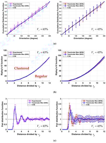
Figure 5.
Comparison of statistical spatial metrics of RVEs: (a) nearest neighbor orientation, (b) Ripley’s K function, and (c) pair distribution function.
3.1.2. Ripley’s K Function
Ripley’s K function [23], also termed the second-order intensity function, is defined as the ratio of points within an arbitrary radius distance to the unit square area in Equation (1) as
where is the area of the window, is the number of all points in the window, and is the distance between points and . Additionally, means an indicator function with a value of 1 if the expression in parentheses is true, and a value of 0 otherwise. Here, is a weight function that represents the ratio of the circumference inside the window to the total circumference of the circle passing through point , centered on point . Ripley’s K function in CSR is expressed in Equation (2).
If the corresponding to any of the points is higher than the of the CSR pattern, it means that the points are clustered. On the other hand, being lower than the CSR pattern indicates that the points are somewhat regular [23]. Figure 5b shows Ripley’s K function of experimental data, RFR, RSE, and CSR according to = 65% and 45%. Here, we divided by the for normalization. It can be seen that the results for experimental data, RFR, and RSE are close to the CSR pattern.
3.1.3. Pair Distribution Function
The pair distribution function, termed radial distribution function, indicates the probability that points will exist in an annular region with an inner diameter and an outer diameter ; it can be written as
Substituting Equation (2) into Equation (3), the pair distribution function of CSR is . Therefore, as increases, the pair distribution function for the fiber distribution approaches 1, indicating that the fiber distribution is randomly arranged [28]. Figure 5c shows the pair distribution function of experimental data, RFR, RSE, and CSR according to = 65% and 45%. The results of the experimental data, RFR, and RSE show that the larger is close to , the CSR pattern. In particular, in the case of = 65%, the results of RSE were almost same to the experimental results. It can be seen that the proposed RVEs are proper to simulate the cross-section of actual fibers.
3.2. Comparison of the Results between Actual Noncircular Fibers and Circular Fibers
In this section, we compared the performance of the proposed RVEs of actual noncircular fibers with conventional RVEs of circular fibers. To generate RVEs consisting of circular fibers, the RFR and RSE algorithms were also used. The minimum distance between fibers used in the RSE algorithm was the same as that of noncircular fibers. Furthermore, the radius of circular fibers was set to . Figure 6 shows the RVE samples of = 45% according to RFR and RSE algorithms with conventional circular fibers and actual noncircular fibers by a shape-library approach.
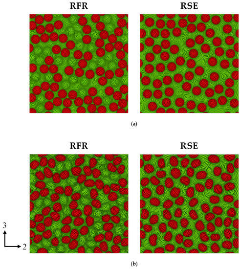
Figure 6.
RVE samples of = 45%: (a) conventional circular approach and (b) shape-library approach.
Table 2 shows the , standard deviation (SD, ), and relative standard deviation (RSD, ) of of the RVE samples corresponding to , and it can be seen that and its corresponding of RVE samples are not exactly identical. In particular, the RVE samples with noncircular fibers show some deviation from those with circular fibers because they have large RSD values in comparison to the RSD values of circular fibers. Given that the volume of each noncircular fiber is not identical, RVE samples with the same cannot be produced. The will be approximately satisfied.
Table 2.
Mean, SD, and RSD of of RVE samples corresponding to .
3.2.1. Comparison of the Effective Elastic Properties
To calculate the effective elastics properties of RVEs, we employed a popular computational homogenization scheme [29] with a set of periodic boundary conditions (PBCs) showing high convergence rate [30] on RVEs. Its details are summarized in Appendix A. As a result, longitudinal modulus , transverse modulus and , out-of-plane shear modulus , in-plane shear modulus , and Poisson’s ratio and were calculated by using Abaqus and MATLAB. Furthermore, for each RFR; RSE algorithm; and noncircular, circular fiber shape, 100 RVEs were used for each . As constituent materials of the composite, two composite materials: M55J/M18 [22] and T300/PR319 [31] were used. Fibers are transversely isotropic materials and matrices are isotropic materials as shown in Table 3. We chose these two materials due to the large difference of the relative ratios of elastic modulus between fiber and matrix defined as
where and . Here, indicates the relative ratio of the longitudinal elastic moduli, and indicates the relative ratio of the transverse elastic moduli.
Table 3.
Elastic properties of fibers and matrices and the relative ratio.
In the case of M55J/M18, the relative ratio of the all transverse moduli, including , , and , are 1.8229, 2.1923, and 14.1314, respectively, which are much lower than those of T300/PR319, such as 15.7895, 19.9184, and 42.6258.
Figure 7 and Figure 8 show the effective elastic properties (, , , ) according to from 5% to 60% of M55J/M18 and T300/PR319 by the computational homogenization, respectively. Figure 9 and Figure 10 show the histogram and normal distribution in terms of and of the effective elastic properties for = 60% of M55J/M18 and T300/PR319, respectively. Table 4 and Table 5 show the and relative error of the effective elastic properties for = 60%, 55%, and 45% of M55J/M18 and T300/PR319, respectively. From the results, it can be seen that both materials show little deviation in , but the deviation of RVE with noncircular fiber is greater than that of RVE with circular fibers as seen in Figure 9a and Figure 10a. This is because the deviation in of RVE with noncircular fiber is larger than that of RVE with circular fiber as discussed in Section 3.2.
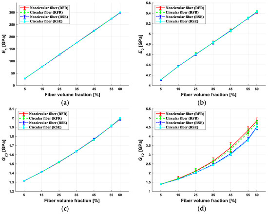
Figure 7.
Effective elastic properties: (a) , (b) , (c) , and (d) of M55J/M18, with ranging from 5% to 60%.
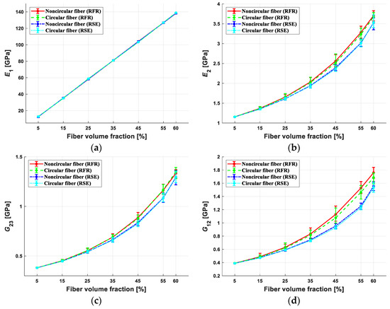
Figure 8.
Effective elastic properties: (a) , (b) , (c) , and (d) of T300/PR319, with ranging from 5% to 60%.
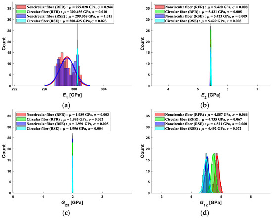
Figure 9.
Effective elastic properties: (a) , (b) , (c) , and (d) of M55J/M18, with .
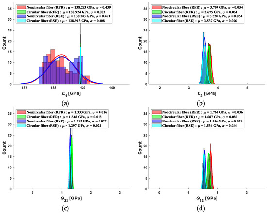
Figure 10.
Effective elastic properties: (a) , (b) , (c) , and (d) of T300/PR319, with .
Table 4.
Comparison of the effective elastic properties of M55J/M18.
Table 5.
Comparison of the effective elastic properties of T300/PR319.
Additionally, it should be noted that, in the case of M55J/M18, the deviations of the transverse moduli , are minimal regardless of the fiber shape and the algorithm of random RVEs. However, the other transverse modulus varies according to the fiber shape and the algorithm of random RVEs. In the case of T300/PR319, all transverse modulus , , and show large deviations according to the RFR and RSE algorithms, and as increases, the deviation increases. For example, for = 60% with the RFR algorithm, the deviation of according to fiber shape is 4.33%, which is larger than that of M55J/M18 (=2.58%). As mentioned earlier, it could be because of the M55J/M18 composite is not significant compared to that of T300/PR319. Although the difference in the effective elastic properties according to the fiber shape of M55J/M18 is small, the actual noncircular fiber shapes should be considered because of the transverse tensile strength accompanying crack propagation. The reason is that, according to our previous work [18], it was reported that the result of the transverse crack propagation simulation showed a different crack pattern from the test result when the circular fibers were assumed instead of the actual fibers. In addition, as of the composite is larger, the deviation of , , and values of RFR are larger than those of RSE. This is because the minimum distance between the fibers of the RFR is closer than that of the RSE, as reported in [24].
To check randomness using the effective elastic properties of RVEs with noncircular fibers in the transverse direction, the symmetry of the compliance matrix was checked as follows:
In addition, the anisotropic ratio was confirmed as follows:
Table 6 shows the results for Equations (5) and (6). It can be seen that all values are close to unity and are sufficiently random in the transverse direction.
Table 6.
Symmetry of the compliance matrix and anisotropic ratio of M55J/M18 and T300/PR319 with noncircular fibers.
3.2.2. Comparison of the Maximum Von Mises Stress in Matrix
In this section, the distribution of the von Mises stress () in the matrix is compared when 1% of the tensile strain is given with PBCs in the transverse direction (2-direction) by using Abaqus. At this time, the stress was calculated at the centroid of the element. Furthermore, as in Section 3.2.1, for each RFR; RSE algorithm; and noncircular, circular fiber shape, 100 RVEs were used for each . Figure 11 shows an example of a contour sample of von Mises stress in the matrix of T300/PR319 with = 60%. Figure 12 and Table 7 show the maximum von Mises stress value in terms of the and error bar in the matrix for diverse of M55J/M18 and T300/PR319, respectively. The results show that the RVE generated by RFR has a higher maximum von Mises stress value in the matrix than those generated by RSE. As mentioned in Section 3.2.1, it is because the minimum distance between the fibers of RFR is smaller than that of the RSE, so that it has larger maximum von Mises stress in the matrix. Furthermore, as the increases, of the maximum von Mises stress tends to increase. However, the variation of is sensitive to the minimum distance between the fibers as reported in other work [32]. In this work, we set the minimum distance of RFR as and and that of RSE as in Table 1. Thus, the trend of the maximum stress could be altered by adjusting the minimum distance.
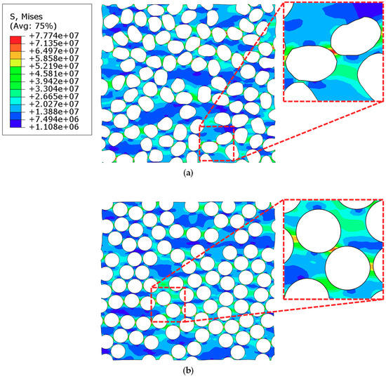
Figure 11.
Von Mises stress with 1% tensile strain for = 60% of T300/PR319: (a) RVEs with noncircular fibers and (b) RVEs with circular fibers.
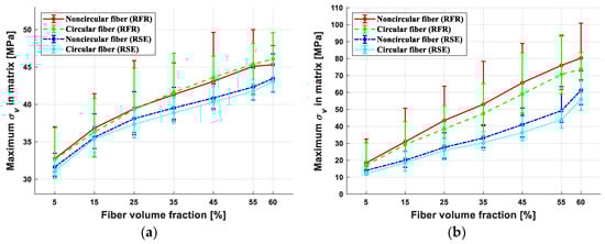
Figure 12.
Comparison of maximum von Mises stress in the matrix for ranging from 5% to 60%: (a) M55J/M18 and (b) T300/PR319.
Table 7.
Comparison of the maximum von Mises stress in matrix.
In addition, as increases (i.e., T300/PR319), the RVE composed of noncircular fibers tends to a larger maximum von Mises stress in the matrix and wider deviation than the RVEs composed of circular fibers. In the case of T300/PR319 with = 60%, the deviations of RFR and RSE according to fiber shape are 8.83%, 9.68%, respectively. Furthermore, it can be seen that the maximum deviation is 12.69% when = 45% with the RSE algorithm in T300/PR319. However, in the case of M55J/M18 with a lower , the maximum deviation of von Mises stress is quite minimal, less than 2%. Thus, it is concluded that the effect of shape on the maximum stress is critical as the is larger.
4. Conclusions
In this work, we generated RVEs considering actual noncircular fibers randomly selected from a particle-shape library, including the features of M55J. The RSE and RFR algorithms were employed to create RVEs various along with proper modification to consider the noncircular fibers.
To check the randomness of the proposed RVEs, we calculated spatial and physical metrics, concluded that the proposed method is sufficiently random, and reproduced experimental data in terms of the shapes and positions of actual fibers. In addition, to investigate the effect of the fiber shapes on the stiffness and strength of the composite, RVEs with circular fibers were also prepared. The material properties of M55J/M18 and T300/PR319 were adopted, and the effective elastic properties were compared. Based on the results, it is concluded that M55J/M18 having a low showed minimal deviation according to the fiber shapes. However, in the case of T300/PR319, which has a high , the maximum deviation of according to the fiber shapes was about 5%. Finally, to investigate the effect on the material fracture strength, the maximum von Mises stress in the matrix was compared with a tensile strain of 1% in the transverse direction according to the fiber shapes. The results showed that the maximum difference according to the fiber shapes of M55J/M18 was up to about 2%, but that of T300/PR319 was up to about 13%. Thus, from a practical point of view, when predicting the strength of composite using micromechanical models having a large of the composites, it is necessary to consider the actual noncircular fiber shapes and positions in the micromechanics model.
Author Contributions
Conceptualization, M.-S.G.; Funding acquisition, D.-S.H.; Supervision, J.H.L.; Writing—original draft, M.-S.G.; Writing—review and editing, M.-S.G., S.-M.P. and D.-W.K. All authors have read and agreed to the published version of the manuscript.
Funding
This research was supported through the National Research Foundation of Korea (NRF) funded by the Ministry of Science and ICT (No. 2020R1F1A1075588). Additionally, this research was supported by “Research Base Construction Fund Support Program” funded by Jeonbuk National University in 2019.
Conflicts of Interest
The authors declare no conflict of interest.
Appendix A. Computational Homogenization Schemes
The stress and strain relationship in a unidirectional lamina is typically expressed as
where , , and are stress, strain, and stiffness matrices in the form of the vector notation, respectively, and is the position vector at an arbitrary point in an RVE.
Due to the transversely isotropic symmetry of the stiffness , it is well known that there are only five independent elastic moduli: , , , , and . In the case of random fiber arrays, due to an anisotropic ratio, one more parameter, , is needed. To determine the elastic properties of unidirectional composites in a theoretical manner, computational homogenization in relation to the present study is briefly summarized.
To predict the equivalent elastic properties of a unidirectional lamina in the computational homogenization scheme, an RVE comprising fibers and a matrix with a predefined fiber-volume ratio is first modeled with a set of FE meshes. Proper periodic boundary conditions in Equation (A2) are then applied to satisfy Hill–Mandel or macro-homogeneity condition [33,34]:
where the superscripts and indicate the positive and negative sides of the RVE in the -direction, respectively. That is, the displacements for each periodic pair are constrained by Equation (A2). In addition, indicates the difference between the coordinates for the periodic pair in the -direction. Only in the case of , corresponds to the length of the RVE with respect to the -direction, i.e., , , , respectively; and the others are zero when the periodic boundary surfaces of the RVE are assumed to be perpendicular to the Cartesian coordinates axes. The prescribed strain imposed on the RVE is denoted by .
We consider six independent macroscopic periodic deformations of the RVE, which correspond to six strain components in the form of vector notation, respectively. First, one of the six strain components, corresponding to the prescribed , is non-zero, while the others are zero. For example, when is prescribed, the corresponding constraints are given as
Then, the FE analysis was conducted imposing the above constraints at all the nodes on boundary surfaces of the RVE. Similarly, the FE analyses for the other five strain components were carried out. For each of the macroscopic periodic deformations, the average stresses can be obtained by
where is the RVE volume. The macroscopic strain–stress relationship in the form of the vector notation is given with the compliance matrix , as follows:
where the macroscopic averaged strain corresponds to the prescribed strain . The compliance matrix can be thus computed from Equations (A5) and (A6). Finally, all elastic moduli are determined by comparing the computed compliance matrix with the compliance matrix of a unidirectional lamina as follows:
References
- Catalanotti, G.; Sebaey, T. An algorithm for the generation of three-dimensional statistically Representative Volume Elements of unidirectional fibre-reinforced plastics: Focusing on the fibres waviness. Compos. Struct. 2019, 227, 111272. [Google Scholar] [CrossRef]
- Herasati, S.; Zhang, L. A new method for characterizing and modeling the waviness and alignment of carbon nanotubes in composites. Compos. Sci. Technol. 2014, 100, 136–142. [Google Scholar] [CrossRef]
- Ahmadian, H.; Yang, M.; Nagarajan, A.; Soghrati, S. Effects of shape and misalignment of fibers on the failure response of carbon fiber reinforced polymers. Comput. Mech. 2019, 63, 999–1017. [Google Scholar] [CrossRef]
- Sebaey, T.; Catalanotti, G.; O’Dowd, N. A microscale integrated approach to measure and model fibre misalignment in fibre-reinforced composites. Compos. Sci. Technol. 2019, 183, 107793. [Google Scholar] [CrossRef]
- Makarov, I.S.; Golova, L.K.; Vinogradov, M.I.; Levin, I.S.; Shandryuk, G.A.; Arkharova, N.A.; Golubev, Y.V.; Berkovich, A.K.; Eremin, T.V.; Obraztsova, E.D. The Effect of Alcohol Precipitants on Structural and Morphological Features and Thermal Properties of Lyocell Fibers. Fibers 2020, 8, 43. [Google Scholar] [CrossRef]
- Peng, S.; Shao, H.; Hu, X. Lyocell fibers as the precursor of carbon fibers. J. Appl. Polym. Sci. 2003, 90, 1941–1947. [Google Scholar] [CrossRef]
- Huang, X. Fabrication and properties of carbon fibers. Materials 2009, 2, 2369–2403. [Google Scholar] [CrossRef]
- Xu, Z.; Huang, Y.; Liu, L.; Zhang, C.; Long, J.; He, J.; Shao, L. Surface characteristics of kidney and circular section carbon fibers and mechanical behavior of composites. Mater. Chem. Phys. 2007, 106, 16–21. [Google Scholar] [CrossRef]
- Kim, T.-J.; Park, C.-K. Flexural and tensile strength developments of various shape carbon fiber-reinforced lightweight cementitious composites. Cem. Concr. Res. 1998, 28, 955–960. [Google Scholar] [CrossRef]
- Park, S.-J.; Seo, M.-K.; Shim, H.-B. Effect of fiber shapes on physical characteristics of non-circular carbon fibers-reinforced composites. Mater. Sci. Eng. A 2003, 352, 34–39. [Google Scholar] [CrossRef]
- Xu, Z.; Li, J.; Wu, X.; Huang, Y.; Chen, L.; Zhang, G. Effect of kidney-type and circular cross sections on carbon fiber surface and composite interface. Compos. Part A Appl. Sci. Manuf. 2008, 39, 301–307. [Google Scholar] [CrossRef]
- Park, S.-J.; Seo, M.-K.; Shim, H.-B.; Rhee, K.-Y. Effect of different cross-section types on mechanical properties of carbon fibers-reinforced cement composites. Mater. Sci. Eng. A 2004, 366, 348–355. [Google Scholar] [CrossRef]
- Yang, L.; Liu, X.; Wu, Z.; Wang, R. Effects of triangle-shape fiber on the transverse mechanical properties of unidirectional carbon fiber reinforced plastics. Compos. Struct. 2016, 152, 617–625. [Google Scholar] [CrossRef]
- Higuchi, R.; Yokozeki, T.; Nagashima, T.; Aoki, T. Evaluation of mechanical properties of noncircular carbon fiber reinforced plastics by using XFEM-based computational micromechanics. Compos. Part A Appl. Sci. Manuf. 2019, 126, 105556. [Google Scholar] [CrossRef]
- Herráez, M.; González, C.; Lopes, C.; de Villoria, R.G.; LLorca, J.; Varela, T.; Sánchez, J. Computational micromechanics evaluation of the effect of fibre shape on the transverse strength of unidirectional composites: An approach to virtual materials design. Compos. Part A Appl. Sci. Manuf. 2016, 91, 484–492. [Google Scholar] [CrossRef]
- Wang, M.; Zhang, P.; Fei, Q.; Guo, F. Computational evaluation of the effects of void on the transverse tensile strengths of unidirectional composites considering thermal residual stress. Compos. Struct. 2019, 227, 111287. [Google Scholar] [CrossRef]
- Liu, X.; Wang, R.; Wu, Z.; Liu, W. The effect of triangle-shape carbon fiber on the flexural properties of the carbon fiber reinforced plastics. Mater. Lett. 2012, 73, 21–23. [Google Scholar] [CrossRef]
- Jeong, G.; Lim, J.H.; Choi, C.; Kim, S.-W. A virtual experimental approach to evaluate transverse damage behavior of a unidirectional composite considering noncircular fiber cross-sections. Compos. Struct. 2019, 111369. [Google Scholar] [CrossRef]
- Park, H.M.; Park, S.; Lee, S.-M.; Shon, I.-J.; Jeon, H.; Yang, B. Automated generation of carbon nanotube morphology in cement composite via data-driven approaches. Compos. Part B Eng. 2019, 167, 51–62. [Google Scholar] [CrossRef]
- You, H.; Kim, Y.; Yun, G.J. Computationally fast morphological descriptor-based microstructure reconstruction algorithms for particulate composites. Compos. Sci. Technol. 2019, 182, 107746. [Google Scholar] [CrossRef]
- Kim, Y.; Yun, G.J. Effects of microstructure morphology on stress in mechanoluminescent particles: Micro CT image-based 3D finite element analyses. Compos. Part A Appl. Sci. Manuf. 2018, 114, 338–351. [Google Scholar] [CrossRef]
- Lim, J.H.; Kim, H.; Kim, S.-W.; Sohn, D. A microstructure modeling scheme for unidirectional composites using signed distance function based boundary smoothing and element trimming. Adv. Eng. Softw. 2017, 109, 1–14. [Google Scholar] [CrossRef]
- Yang, L.; Yan, Y.; Ran, Z.; Liu, Y. A new method for generating random fibre distributions for fibre reinforced composites. Compos. Sci. Technol. 2013, 76, 14–20. [Google Scholar] [CrossRef]
- Park, S.-M.; Lim, J.H.; Seong, M.R.; Sohn, D. Efficient generator of random fiber distribution with diverse volume fractions by random fiber removal. Compos. Part B Eng. 2019, 167, 302–316. [Google Scholar] [CrossRef]
- Kim, D.-W.; Lim, J.H.; Yu, J. Efficient prediction of the electrical conductivity and percolation threshold of nanocomposite containing spherical particles with three-dimensional random representative volume elements by random filler removal. Compos. Part B Eng. 2019, 168, 387–397. [Google Scholar] [CrossRef]
- González, C.; LLorca, J. Mechanical behavior of unidirectional fiber-reinforced polymers under transverse compression: Microscopic mechanisms and modeling. Compos. Sci. Technol. 2007, 67, 2795–2806. [Google Scholar] [CrossRef]
- Illian, J.; Penttinen, A.; Stoyan, H.; Stoyan, D. Statistical Analysis and Modelling of Spatial Point Patterns; John Wiley Sons: Hoboken, NJ, USA, 2008. [Google Scholar]
- Melro, A.; Camanho, P.; Pinho, S. Generation of random distribution of fibres in long-fibre reinforced composites. Compos. Sci. Technol. 2008, 68, 2092–2102. [Google Scholar] [CrossRef]
- Matouš, K.; Geers, M.G.; Kouznetsova, V.G.; Gillman, A. A review of predictive nonlinear theories for multiscale modeling of heterogeneous materials. J. Comput. Phys. 2017, 330, 192–220. [Google Scholar] [CrossRef]
- Nguyen, V.-D.; Béchet, E.; Geuzaine, C.; Noels, L. Imposing periodic boundary condition on arbitrary meshes by polynomial interpolation. Comput. Mater. Sci. 2012, 55, 390–406. [Google Scholar] [CrossRef]
- Huang, Z.-M. On micromechanics approach to stiffness and strength of unidirectional composites. J. Reinf. Plast. Compos. 2019, 38, 167–196. [Google Scholar] [CrossRef]
- Ghayoor, H.; Hoa, S.V.; Marsden, C.C. A micromechanical study of stress concentrations in composites. Compos. Part B Eng. 2018, 132, 115–124. [Google Scholar] [CrossRef]
- Hill, R. Elastic properties of reinforced solids: Some theoretical principles. J. Mech. Phys. Solids 1963, 11, 357–372. [Google Scholar] [CrossRef]
- Mandel, J. Contribution théorique à l’étude de l’écrouissage et des lois de l’écoulement plastique. In Applied Mechanics; Springer: Berlin/Heidelberg, Germany, 1966; pp. 502–509. [Google Scholar]


© 2020 by the authors. Licensee MDPI, Basel, Switzerland. This article is an open access article distributed under the terms and conditions of the Creative Commons Attribution (CC BY) license (http://creativecommons.org/licenses/by/4.0/).