Characterization of Localized Atmospheric Turbulence Layer Using Laser Light Backscattered off Moving Target

Abstract

A concept of atmospheric turbulence characterization using laser light backscattered off a moving unresolved target or a moving target with a glint is considered and analyzed through wave-optics numerical simulations. The technique is based on analysis of the autocorrelation function and variance of the power signal measured by the target-in-the-loop atmospheric sensing (TILAS) system composed of a single-mode-fiber-based optical transceiver and the moving target. It is shown that the TILAS received power signal autocorrelation function strongly depends on the turbulence distribution and is weakly sensitive to the turbulence strength, while the signal variance equally depends on these parameters. Assuming the atmospheric turbulence model can be represented by a single spatially localized turbulence layer and the target position and speed are known independently, consecutive analysis of the autocorrelation function and variance of the TILAS signal allows evaluation of both the turbulence layer strength and position along the optical propagation path. It is also demonstrated that the autocorrelation function can potentially be used for the atmospheric turbulence outer scale estimation.

1. Introduction

Atmospheric turbulence characterization based on remote sensing of the target-plane laser beam characteristics is typically performed along the optical propagation path between optical transceiver and a target. Assuming the turbulence is uniform (homogeneous) and described by the Kolmogorov power spectrum [1], these characteristics can then be used to estimate the refractive index structure parameter $C_n^2$ averaged over the target line of sight. However, in many cases, atmospheric turbulence is non-uniform [2] and composed of relatively thin, horizontally extended layers of high values of the refractive index caused, e.g., by evening transition of the boundary layer [3] or jet streams and gravity waves in the upper troposphere and lower stratosphere [4]. These layers have frequently been observed with balloons [5] and radars [6]. The knowledge of atmospheric turbulence layer characteristics, such as their strength and position along the optical propagation path, is important for improving the efficiency of laser systems in beam projection and free-space optical communication applications using, e.g., multi-conjugate adaptive optics technique [7].

In this paper, we present a concept which allows characterization of atmospheric turbulence layers along the trajectory of a moving target as well as real-time evaluation of major laser beam characteristics such as intensity scintillations directly on the remote target. The technique is based on the previously developed target-in-the-loop atmospheric sensing (TILAS) concept [8], which was experimentally proven over a 7-km atmospheric propagation path to a stationary retro-target [9]. Here, we consider a more general case when the TILAS system, a single-mode-fiber-based optical transceiver, is operating with a moving target. As shown in the paper, the use of the moving target offers several advantages for atmospheric characterization such as estimation of strength and position of a spatially localized turbulence layer, as well as evaluation of the turbulence outer scale L₀, based on analysis of both the autocorrelation function and variance of the power signal measured by the TILAS system.

The principal assumptions required for the TILAS technique presented here are as follows. First, the target is supposed to either be unresolved (smaller than the diffraction-limited beam footprint at the target plane), have a glint caused by reflection from the target’s surface, or have a small-size retro-reflector attached. It is also presumed that the distance to the target as well as the target’s speed are known. Besides, we utilize the Taylors’ frozen turbulence hypothesis and assume that the target is moving sufficiently fast, so that we may neglect the impact of the wind along the propagation path.

The paper is organized as follows. A concept of the TILAS system operating with a moving target with a glint is described in Section 2. Numerical simulation approach for modeling and simulation of the TILAS system is detailed in Section 3. Numerical simulation results are discussed in Section 4. The paper concludes with a summary and suggestions for future work.

2. Target-in-the-Loop Atmospheric Sensing Concept

The theoretical foundation of the TILAS concept is based on the optical reciprocity principle [10] and the associated conservation law for the so-called interference metric J_int coupling the complex amplitudes of the counter-propagating optical waves [11,12,13]. As was recently shown [8,9,14], the square modulus of the interference metric can be measured using the TILAS system depicted in Figure 1a. This system is composed of a laser, fiber-optics circulator, fiber-coupled transceiver, and fiber-coupled photodetector. The circulator separates the outgoing and incoming laser beams by sending the outgoing, linearly-polarized Gaussian beam from the laser to the transceiver, while the entering wave is directed to the photodetector. The power signal measured at the TILAS photodetector is given by the expression [8]

$$P_{\mathrm{TILAS}}(t)=\alpha {\left|J_{\mathrm{int}}(t)\right|}^2=\alpha {\left|{\displaystyle \int A(r,z=0)\psi (r,z=0,t)d^{2}r}\right|}^2.$$

(1)

where α is a coefficient dependent on the transmitted power and the photodetector’s sensitivity, $A(r,z=0)$ is the stationary complex amplitude of the outgoing wave transmitted along the optical z-axis, $\psi (r,z=0,t)$ is the amplitude of the incoming wave backscattered off a target located at the plane z = L back to the receiver (transceiver) plane z = 0, r = {x, y} is the spatial vector in the plane orthogonal to the propagation direction, t is the time, and the integration is performed over the entire transverse plane.

In this paper, we consider the stationary TILAS transceiver and the target with a glint, moving perpendicularly to the sensing path direction with velocity $v_T$ (Figure 1b). For this type of target, the following quantities are computed based on the TILAS received power signal measurements:

1.

Autocorrelation function of the signal,

$$B(\tau )=\frac{\langle P_{\mathrm{TILAS}}(t)P_{\mathrm{TILAS}}(t+\tau )\rangle -{\langle P_{\mathrm{TILAS}}(t)\rangle }^2}{\langle P_{\mathrm{TILAS}}^2(t)\rangle -{\langle P_{\mathrm{TILAS}}(t)\rangle }^2},$$

(2)

where τ is the time delay between the power signal values measured at different moments of time t and angle brackets denote the averaging over the integration time interval T. Here we assume that $T\gg {\tau }_{\mathrm{at}}$, where τ_at is the characteristic correlation time of the atmospheric turbulence pattern change inside the transceiver aperture [8].

2.

Interference metric variance, also referred to here as the TILAS received power signal variance, given by the expression [8]

$${\sigma }_J^2={\langle P_{\mathrm{TILAS}}(t)\rangle }_T/{\langle \sqrt{P_{\mathrm{TILAS}}(t)}\rangle }_T^2-1.$$

(3)

In this paper, we focus on the atmospheric turbulence model that can be represented by a single spatially localized turbulence layer, referred to as here as the single layer model. The homogeneously distributed turbulence model is also briefly considered. We show that parameters B(τ) and ${\sigma }_J^2$ given by the equations above can be used for estimation of both the strength and position of the turbulence layer along the optical propagation path, and, potentially, can lead to the turbulence profiling. We also demonstrate that consecutive analysis of the correlation properties of the TILAS received power signal P_TILAS (t) results in the estimation of the atmospheric turbulence outer scale L₀ of the layer.

Numerical simulation approach for the analysis is explained in the following section.

3. Numerical Simulation Approach and Settings

Our approach is based on direct numerical integration of the parabolic wave equation (the so-called wave-optics technique). This integration is performed using the split-step operator method [15,16,17], where the turbulence-induced refractive index perturbations along the propagation path of length L are represented by a set of thin, two-dimensional (2D), statistically independent phase screens.

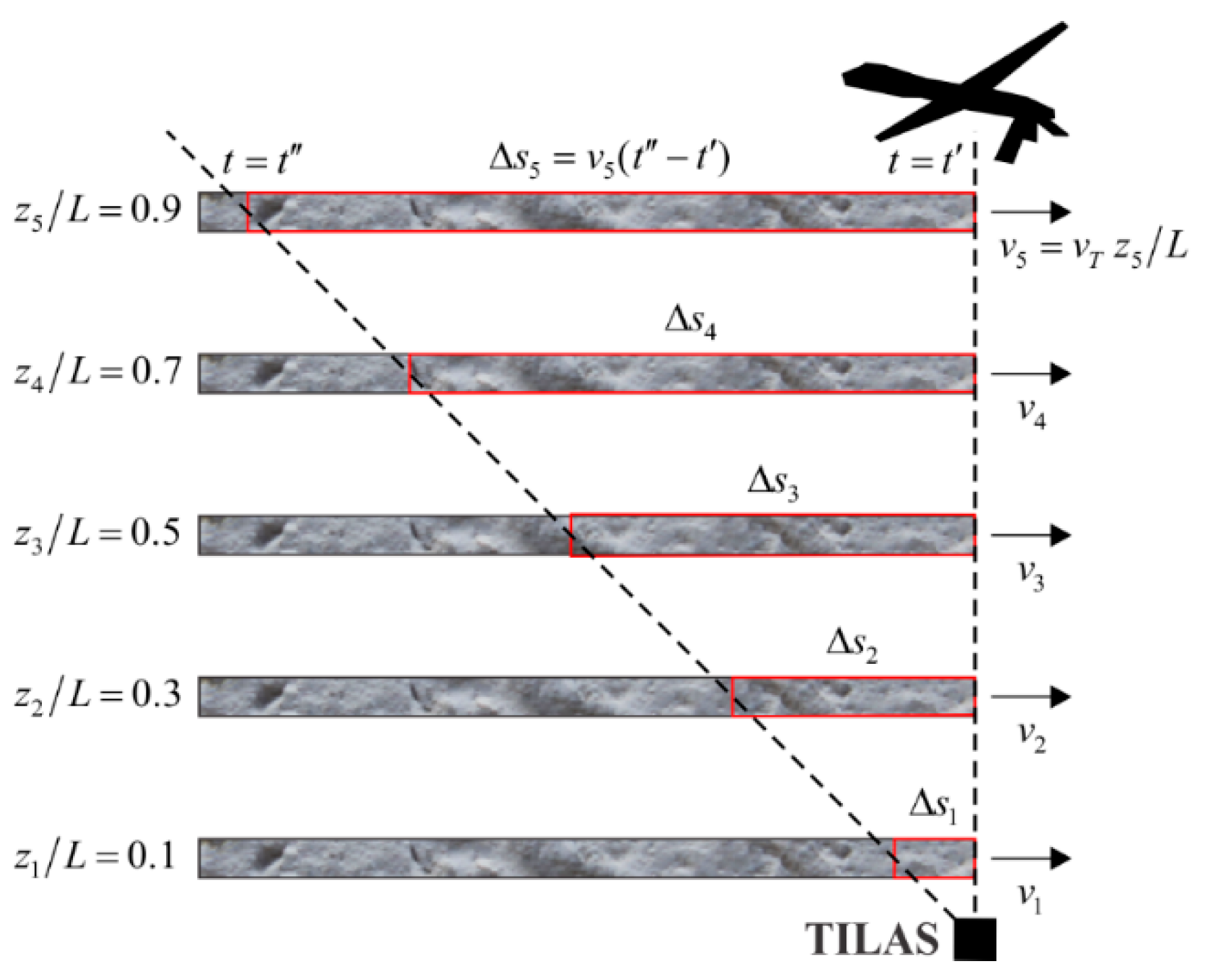
In our simulations, the number of phase screens M is varied from one for the single layer model to five for the distributed turbulence model. For the single layer model, the screens are positioned at five selected distances from the TILAS transceiver, while for the distributed turbulence model, they are distributed equidistantly along the propagation path at distances $z_j=\Delta z(2j-1)/2$, where $\Delta z=L/M$ is the layer width and j = 1, …, M. The latter case is illustrated in Figure 2 for M = 5.

The turbulence strength is defined by the refractive index structure parameter $C_n^2(z)$; the corresponding plane-wave Fried parameter computed over the distance L is given by $r_0={\{0.423k^2{\int }_0^L{C}_n^2(z)dz\}}^{-3/5}$ [18], where $k=2\pi /\lambda$ is the wavenumber. For the phase screen located at $z=z_j$, the Fried parameter is correspondingly defined as $r_0^{(j)}={\{0.423k^2{\int }_{z_j-\Delta z/2}^{z_j+\Delta z/2}{C}_n^2(z)dz\}}^{-3/5}$ [19]. For the single layer model, we suppose that $C_n^2(z)=\mathrm{const}$ withing the layer of width Δz and zero otherwise, i.e., $r_0=1.68{(k^2{C}_n^2\Delta z)}^{-3/5}=r_0^{(j)}$. For the distributed turbulence model, we assume that the turbulence is homogeneous, which is a commonly used assumption for relatively short or nearly horizontal propagation paths [18]. In this case, $C_n^2(z)=\mathrm{const}$ along the entire path and $r_0=1.68{(k^2{C}_n^{2}L)}^{-3/5}=r_0^{(j)}{M}^{-3/5}$. For fair comparison of the results obtained for the single layer model with those for the distributed turbulence model, which corresponds to the same value of r₀ for both models, the refractive index structure parameter values for the single layer model are M-fold higher than those for the distributed turbulence model.

In our simulations of the single layer model, the layer width is fixed at $\Delta z=L/5$ and the turbulence strength $C_n^2$ is varied in the interval ${10}^{-16}{\mathrm{m}}^{-2/3}\le C_n^2\le {10}^{-14}{\mathrm{m}}^{-2/3}$. The Fried parameter is respectively ranging from 65 cm to 4.1 cm. For the distributed turbulence model, the corresponding $C_n^2$ values are decreased five times.

To simulate a target moving with the speed $v_T=\left|v_T\right|$ relative to a stationary laser platform with the TILAS sensor, the position of the target is fixed but the jth phase screen is shifted in the opposite direction with the speed $v_j=v_T{z}_j/L$. Over the time interval $\Delta t=t^{″}-t^{\prime }$, this corresponds to the shift distance $\Delta s_j=v_j\Delta t$, as illustrated in Figure 2. Thus, during the same time, screens located at different positions along the path are shifted different distances.

To model engagements involving moving targets, the technique for generation of infinitely-long phase screens [20] is used. The phase screens are assumed to obey the von Karman power spectrum law; it allows us to vary the value of the turbulence outer scale L₀. Note that the use of infinitely-long phase screens permits extending the range of L₀ values beyond the numerical simulation area size (up to four times the size).

As the TILAS outgoing beam, a collimated Gaussian beam with fixed wavelength λ = 1.064 µm and radius W₀ = 1.5 cm, truncated by the circular aperture of diameters d_TILAS = 3.3 cm and 7 cm is considered. The propagation distance to the target is fixed at L = 7 km. The target’s glint is modeled by the circular retro-reflector of diameter d_T = 1 cm. Note that for the set of the parameters selected, d_T is smaller than the diffraction-limited target-plane beam footprint radius $W=W_0{[1+{(2L/k{W}_0^2)}^2]}^{1/2}\simeq 16\mathrm{cm}$, i.e., the retro-reflector is unresolved. The target speed relative to the TILAS system platform with the TILAS sensor is set to $v_T=200\mathrm{m}/\mathrm{s}$.

All computations are performed using numerical grids with resolution of 2048 × 2048 pixels; the simulation area width and sampling size are fixed at 4.096 m and 2 mm, respectively, to meet sampling requirements [21]. The sampling time, i.e., the time between the consecutive phase screen shifts, is fixed at 0.1 ms. The integration interval T is chosen to be equal to 5 s. During this time, the target moves over a distance of 1 km; this results in about 70-m propagation distance change, which is insignificant compared to L = 7 km and can be neglected. At the same time, as mentioned earlier, this interval should exceed the characteristic correlation time τ_at, which can be estimated for the jth screen as ${\tau }_{\mathrm{at}}^{(j)}={\rho }_0^{(j)}/v_j$, where ${\rho }_0^{(j)}$ is the jth screen’s phase fluctuations correlation length, also known as the Tatarskii parameter for spherical wave [22]. Assuming the turbulence layer of width Δz = 1.4 km is located at z = 0.1 L = 0.7 km (closest to the TILAS transceiver aperture) and moving with the speed $v=0.1v_T=20\mathrm{m}/\mathrm{s}$, τ_at ≈ 28 ms for $C_n^2=1\times {10}^{-16}{\mathrm{m}}^{-2/3}$ and 1.7 ms for $C_n^2=1\times {10}^{-14}{\mathrm{m}}^{-2/3}$, which means that the condition $T\gg {\tau }_{\mathrm{at}}$ is satisfied.

The results of our numerical simulations are presented and discussed in the following section.

4. Numerical Simulation Results and Analysis

4.1. Correlation Properties of TILAS Received Power Signal

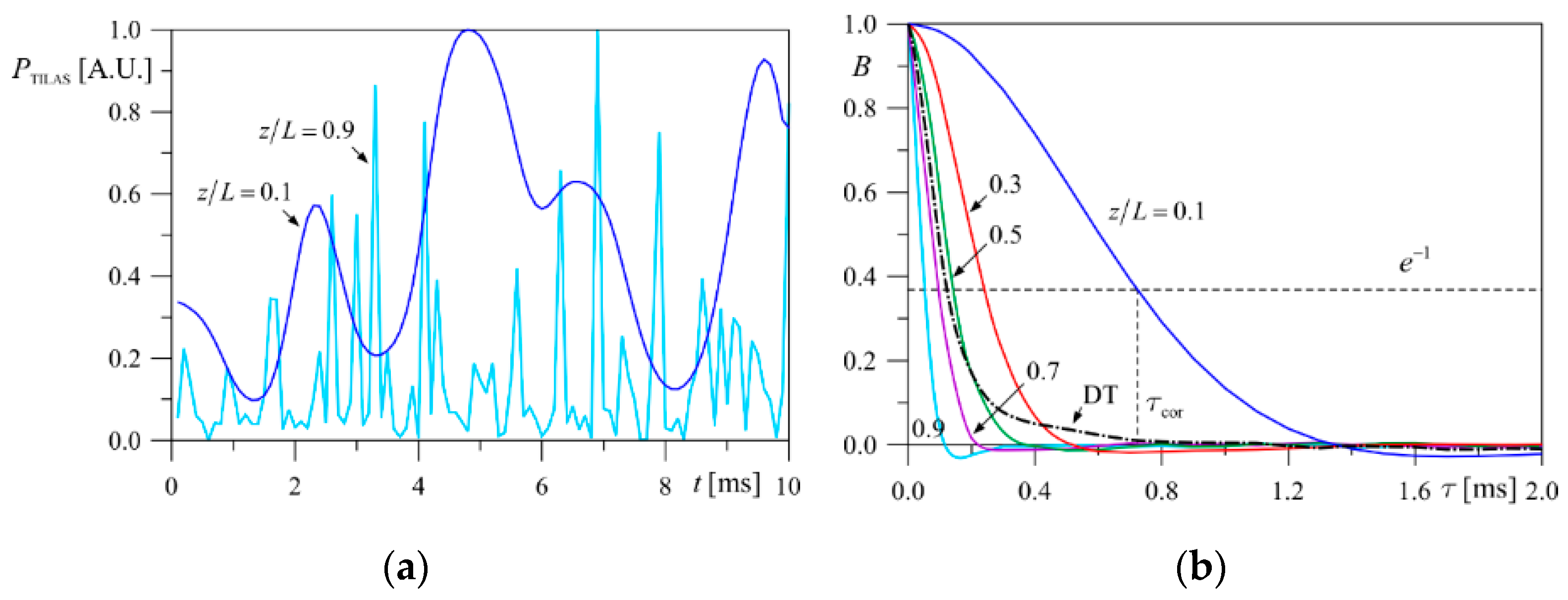
Consider first the correlation properties of the TILAS received power signal P_TILAS (t) for the single layer model, where the turbulence layer of a fixed strength is placed at different distances from the TILAS transceiver. Figure 3a shows the time series of P_TILAS (t) computed over a 10-ms time interval with 0.1-ms sampling time for two different relative positions of the layer between the TILAS transceiver and the moving target, z/L = 0.1 (closer to TILAS) and z/L = 0.9 (closer to the target), characterized by the same Fried radius r₀ = 4.1 cm and turbulence outer scale L₀ = 4 m. As can be seen from Figure 3a, the signal obtained for the case of the turbulence layer located closer to the transceiver (blue line) is changing slower than that for the layer located near the target (sky-blue line). This can be explained by the fact that the turbulence-induced refractive index inhomogeneities inside the propagating beam footprint are updated faster when the layer is located farther from the TILAS transceiver aperture, or closer to the moving target. This happens because during the same time interval, the laser beam following the target would scan sections of different length for layers positioned at different distances from TILAS (see Figure 2).

Typical dependencies of the autocorrelation functions B (Equation (2)) on the time delay τ computed for five different turbulence layer positions ranging from z = 0.1 L to z = 0.9 L with the step of 0.2 L are shown in Figure 3b. Note that the autocorrelation functions B(τ) have Gaussian-like shape, which allows us to directly determine their width by the drop in the function level by a factor exp(−1) ≈ 0.37 compared with B(τ = 0). This width is referred to here as the correlation time, τ_cor. As seen, the correlation time depends on the position of the turbulence layer along the propagation path from the TILAS transceiver to the moving target. The autocorrelation function corresponded to the turbulence layer located near the moving target is characterized by the smallest correlation time while B(τ) related to the layer near the transceiver has the largest τ_cor.

Consider now the distributed turbulence model characterized by the same Fried radius equal to 4.1 cm ($C_n^2=2\times {10}^{-15}{\mathrm{m}}^{-2/3}$). The corresponding autocorrelation function is shown in Figure 3b by the dash-dotted black line. As can be seen from the figure, the distributed turbulence correlation time defined at B(τ) ≈ 0.37 lies between ${\tau }_{\mathrm{cor}}(z/L=0.7)$ and ${\tau }_{\mathrm{cor}}(z/L=0.5)$ defined using the single layer model. However, the distributed turbulence autocorrelation function has a unique shape with a specific slow-decline region at the function’s tail (a ‘pedestal’ or a ‘base’), which is distinct from the Gaussian-like shape of the autocorrelation function computed for the single layer model. This means that the presence of such a base can serve as an indication of the turbulence being distributed, or at least of the presence of more than one turbulence layer along the propagation path.

4.2. Estimation of Turbulence Layer Position Based on TILAS Measurements

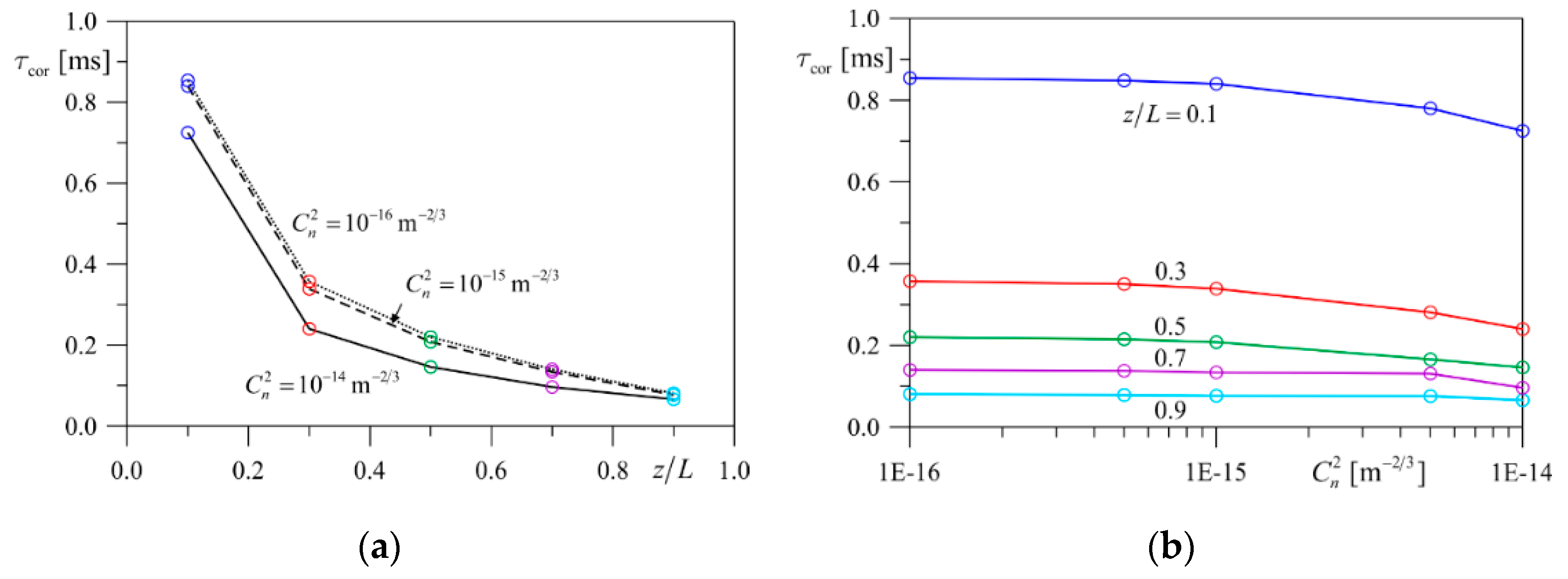
Figure 4a shows the correlation time τ_cor values as functions of the relative position z/L of a single spatially localized turbulence layer, computed for different turbulence strength values varied in the interval ${10}^{-16}{\mathrm{m}}^{-2/3}\le C_n^2\le {10}^{-14}{\mathrm{m}}^{-2/3}$. These plots confirm that the correlation time is sensitive to the layer position; the farther the layer from the TILAS transceiver, the smaller the correlation time. At the same time, the correlation time appears to be weakly dependent on the turbulence layer strength $C_n^2$, as demonstrated in Figure 4b.

Further analysis reveals that the τ_cor curves stay qualitatively the same for different parameters of both the TILAS system and the moving target. Estimations of τ_cor performed with the increased diameter of the TILAS transceiver aperture, d_TILAS = 7 cm, demonstrate comparable monotonically decreasing dependencies τ_cor (z/L) as in Figure 4a, although the absolute values of τ_cor are generally larger for larger d_TILAS. Similar observations are made for the target speed $v_T$; τ_cor is simply inversely proportional to $v_T$. Thus, assuming both the TILAS and the target parameters including the distance to the target and target speed are known, the correlation time τ_cor, which is computed using the autocorrelation function B(τ) of the received power signal P_TILAS (t) measured by the TILAS system, can be used to estimate the position of the turbulence layer. The accuracy of this estimation is somewhat reduced by the dependence of τ_cor on the turbulence strength.

4.3. Estimation of Turbulence Layer Strength Based on TILAS Measurements

Consider analogous dependencies of the TILAS received power signal variance ${\sigma }_J^2$ (Equation (3))on the turbulence layer position (Figure 5a), as well as the turbulence layer strength (Figure 5b). As seen, ${\sigma }_J^2$ demonstrates comparable level of variability for both z/L and $C_n^2$. Besides, the function ${\sigma }_J^2(z/L)$ in Figure 5a is not monotonic; strongest signal fluctuations correspond to the turbulence layer placed in the middle of the propagation path. Therefore, the power signal variance is not suitable to be used to define the layer position. However, ${\sigma }_J^2(C_n^2)$ in Figure 5b is monotonically increasing with the increase of the turbulence strength (at least inside the examined interval of $C_n^2$). At the same time, as was confirmed by our numerical analysis, this variance does not depend on the speed of the target, $v_T$. Therefore, if the turbulence layer position z/L is already defined from the correlation times estimations and the TILAS parameters and the distance to the target are known independently, the set of functions ${\sigma }_J^2(C_n^2)$ computed for different layer positions can be used for retrieval of the turbulence layer strength.

The value of the TILAS received power signal variance for the distributed turbulence case with $C_n^2=2\times {10}^{-15}{\mathrm{m}}^{-2/3}$ and the same Fried parameter as for the single layer model with $C_n^2={10}^{-14}{\mathrm{m}}^{-2/3}$ is close to those obtained for the turbulence layer placed around 0.3 z/L or 0.7 z/L (see dash-dotted and solid lines in Figure 5a). This suggests that the layers positioned close to the middle of the propagation path contribute the most to the power signal variance.

4.4. Evaluation of Turbulence Layer Outer Scale Based on TILAS Measurements

In this work, the possibility of direct evaluation of the atmospheric-turbulence outer scale L₀ using TILAS measurements and autocorrelation function analysis is investigated. This possibility can help to resolve a long-standing problem of sensing of the so-called piston phase (optical path difference) [23], which, within the framework of the Kolmogorov turbulence theory, is associated with the outer scale. This is essential, e.g., for long-range electro-optical systems based on coherent detection techniques [24].

Typical autocorrelation functions B(τ) computed in the presence of a single turbulence layer of strength $C_n^2={10}^{-15}{\mathrm{m}}^{-2/3}$ (r₀ = 16.3 cm) characterized by the turbulence outer scale values L₀ varied from 0.25 m (dotted lines) to 16 m (solid lines) are shown in Figure 6. Here, the TILAS transceiver aperture diameter is fixed at d_TILAS = 7 cm; for the TILAS aperture size d_TILAS = 3.3 cm considered in previous sections, the functions dependence on the outer scale is less evident. Analysis of shapes of these functions reveals that the B(τ) decline rate increases with the decrease of L₀. Besides, if the outer scales are small enough, the negative correlation may be observed. The impact of L₀ seems to be more pronounced on the functions computed for layers located closer to the TILAS transceiver (compare Figure 6a for z/L = 0.1 (near TILAS) and Figure 6b for z/L = 0.3); for turbulence layers that are closer to the target, the width of the autocorrelation functions (i.e., the correlation time τ_cor) becomes nearly indifferent to the turbulence outer scale. To increase the sensitivity of τ_cor to L₀, the correlation time can be re-defined, e.g., by the drop in the intensity level by a factor exp(−2) ≈ 0.14. Alternatively, the size of the transceiver aperture diameter can be further increased; as mentioned in Section 4.2, the values of τ_cor increase with the increase of d_TILAS, which helps to differentiate the curves with different values of L₀. Thus, the correlation time can be used to estimate the turbulence outer scale if the layer position and strength are already known.

5. Discussion and Conclusions

Dependence of the autocorrelation function B(τ) and the variance of the TILAS received power signal ${\sigma }_J^2$ on the atmospheric turbulence distribution, strength, and outer scale can serve for turbulence characterization. Sequential analysis of these quantities provides information about the turbulence properties along the laser beam propagation path. Analysis of the shape of the autocorrelation function allows distinguishing between homogeneous and inhomogeneous turbulence distributions, while estimation of the strength of homogeneous turbulence or localized layer can be performed based on the signal variance when the turbulence distribution is known.

The procedure of finding the position and strength of a single turbulence layer based on the τ_cor and ${\sigma }_J^2$ quantities obtained using the TILAS received power signal measurements can be summarized by the following algorithm:

Step 1.

The relative turbulence layer position z/L is estimated using the set of functions τ_cor (z/L) computed for given TILAS parameters, known distance to the target and target speed, as well as various turbulence strengths of the layer $C_n^2$, as in Figure 4a. Since the functions τ_cor (z/L) are weakly dependent on the turbulence strength, the turbulence layer position will be estimated with some error due to the uncertainty of $C_n^2$.

Step 2.

The turbulence layer strength is defined using the set of functions ${\sigma }_J^2(C_n^2)$ computed for the estimated interval of z/L values, as in Figure 5b. The error in the layer position will introduce the corresponding error in the turbulence layer strength estimates.

To reduce the estimation errors, the algorithm can be iterated using the obtained turbulence strength interval as the initial $C_n^2$ interval in Step 1 until the desired accuracy is achieved. To speed up the turbulence layer position and strength retrieval procedure, a set of functions τ_cor (z/L) and ${\sigma }_J^2(C_n^2)$ can be precomputed.

Three examples of the evaluation of the turbulence layer characteristics are given in

Table 1. Examples of turbulence layer characterization

z/L	${\mathit{C}}_{\mathit{n}}^2{[\mathbf{m}}^{-2/3}]$	${\mathit{\tau }}_{\mathbf{cor}}[\mathbf{ms}]$	${\mathit{\sigma }}_{\mathit{J}}^2$	z/L Estimate after 1st Iteration	${\mathit{C}}_{\mathit{n}}^2$$\mathbf{Estimate}\mathbf{after}1\mathbf{st}\mathbf{Iteration}{[\mathbf{m}}^{-2/3}]$	z/L Estimate after 2nd Iteration	${\mathit{C}}_{\mathit{n}}^2$$\mathbf{Estimate}\mathbf{after}2\mathbf{nd}\mathbf{Iteration}{[\mathbf{m}}^{-2/3}]$
0.1	1×10−14	0.73	0.268	[0.10; 0.15]	[0.6; 1.0] × 10−14	[0.10; 0.12]	[0.8; 1.0] × 10−14
0.5	1×10−15	0.21	0.097	[0.36; 0.51]	[0.9; 1.0] × 10−15	[0.49; 0.51]	[0.9; 1.0] × 10−15
0.9	1×10−16	0.08	0.004	[0.83; 0.90]	[0.7; 1.0] × 10−16	[0.88; 0.90]	[0.8; 1.0] × 10−16

. The first two columns show the input parameters used for simulations. The third and fourth columns contain the quantities computed using the TILAS power signal processing, which are used to estimate z/L and $C_n^2$ of a single turbulence layer. The fifth and sixth columns show the intervals of values for the layer position and strength computed after the first iteration of the algorithm. Note that the identification of the layer position appears to be more accurate for layers located on the ends of the propagation path, while the estimation of the layer strength is more accurate for layers located in the middle of the optical path. The second iteration results in noticeable increase of the accuracy, as can be seen by comparing the estimates (last two columns) to the input parameters (first two columns).

More rigorous analysis based on simultaneous evaluation of strength and positions of few layers performed with summarizing autocorrelation function with weight coefficients regarding their position and strength can potentially provide detailed information about complex turbulence distribution. Additional opportunities are related to the use of a multi-aperture TILAS transceiver system. Such a system can transmit several laser beams with different initial diameters, which would serve for estimation of the turbulence outer scale.

References

1. Kolmogorov, A.N. The local structure of turbulence in incompressible viscous fluid for very large Reynolds numbers. Dokl. Akad. Nauk SSSR 1941, 30, 299–303. [Google Scholar]
2. Mahrt, L. Stratified atmospheric boundary layers. Bound. Layer Meteorol. 1999, 90, 375–396. [Google Scholar] [CrossRef]
3. Poulos, G.S.; Blumen, W.; Fritts, D.C.; Lundquist, J.K.; Sun, J.; Burns, S.P.; Nappo, C.; Banta, R.; Newsom, R.; Cuxart, J.; et al. CASES-99: A comprehensive investigation of the stable nocturnal boundary layer. Bull. Am. Meteorol. Soc. 2002, 83, 555–581. [Google Scholar] [CrossRef]
4. Mahalov, A.; Moustaoui, M. Characterization of atmospheric optical turbulence for laser propagation. Laser Photonics Rev. 2010, 4, 144–159. [Google Scholar] [CrossRef]
5. Azouit, M.; Vernin, J. Optical turbulence profiling with balloons relevant to astronomy and atmospheric physics. Publ. Astron. Soc. Pac. 2005, 117, 536–543. [Google Scholar] [CrossRef]
6. Ince, T.; Frasier, S.J.; Muschinski, A.; Pazmany, A.L. An S-band frequency-modulated continuous-wave boundary layer profiler: Description and initial results. Radio Sci. 2003, 38, 1072. [Google Scholar] [CrossRef]
7. Beckers, J.M. Adaptive optics for astronomy: Principles, performance, and applications. Annu. Rev. Astron. Astrophys. 1993, 31, 13–62. [Google Scholar] [CrossRef]
8. Vorontsov, M.A.; Lachinova, S.L.; Majumdar, A.K. Target-in-the-loop remote sensing of laser beam and atmospheric turbulence characteristics. Appl. Opt. 2016, 55, 5172–5179. [Google Scholar] [CrossRef] [PubMed]
9. Polnau, E.; Vorontsov, M.A.; Gudimetla, R. Experimental demonstration of target-in-the-loop remote sensing of laser beam and atmospheric turbulence characteristics. J. Opt. 2019, 21, 095602. [Google Scholar] [CrossRef]
10. Shapiro, J.H. Reciprocity of the turbulent atmosphere. J. Opt. Soc. Am. 1971, 61, 492–495. [Google Scholar] [CrossRef]
11. Vorontsov, M.A.; Shmal’gauzen, V.I. Interference criteria for the focusing of light. Kvant. Elektron. 1980, 7, 500–505. [Google Scholar] [CrossRef]
12. Vorontsov, M.A.; Kolosov, V.V.; Kohnle, A. Adaptive laser beam projection on an extended target: Phase- and field-conjugate precompensation. J. Opt. Soc. Am. A 2007, 24, 1975–1993. [Google Scholar] [CrossRef] [PubMed]
13. Vorontsov, M.A. Conservation laws for counter-propagating optical waves in atmospheric turbulence with application to directed energy and laser communications. In Imaging and Applied Optics, Proceedings of the Propagation Through and Characterization of Distributed Volume Turbulence, Arlington, VA, USA, 23–27 June 2013; Optical Society of America: Arlington, VA, USA, 2013; p. 31. [Google Scholar] [CrossRef]
14. Minet, J.; Vorontsov, M.A.; Polnau, E.; Dolfi, D. Enhanced correlation of received power-signal fluctuations in bidirectional optical links. J. Opt. 2013, 15, 022401. [Google Scholar] [CrossRef]
15. Fleck, J.A.; Morris, J.R.; Feit, M.D. Time-dependent propagation of high-energy laser beams through the atmosphere. Appl. Phys. 1976, 10, 129–160. [Google Scholar] [CrossRef]
16. Martin, J.M.; Flatte, S.M. Intensity images and statistics from numerical simulation of wave propagation in 3-D random media. Appl. Opt. 1988, 27, 2111–2126. [Google Scholar] [CrossRef] [PubMed]
17. Schmidt, J.D. Numerical Simulation of Optical Wave Propagation with Examples in MATLAB. In Press Monograph Series; SPIE Press: Bellingham, WA, USA, 2010; Volume PM199, p. 212. [Google Scholar]
18. Andrews, L.C.; Phillips, R.L. Laser Beam Propagation Through Random Media. In Press Monograph Series; SPIE Press: Bellingham, WA, USA, 1998; Volume PM53. [Google Scholar]
19. Roggemann, M.C.; Welsh, B. Imaging Through Turbulence; CRC Press: Boca Raton, FL, USA, 1996. [Google Scholar]
20. Vorontsov, A.M.; Paramonov, P.V.; Valley, M.T.; Vorontsov, M.A. Generation of infinitely long phase screens for modeling of optical wave propagation in atmospheric turbulence. Waves Random Complex Media 2008, 18, 91–108. [Google Scholar] [CrossRef]
21. Voelz, D.G.; Roggemann, M.C. Digital simulation of scalar optical diffraction: Revisiting chirp function sampling criteria and consequences. Appl. Opt. 2009, 48, 6132–6142. [Google Scholar] [CrossRef] [PubMed]
22. Tatarski, V.I. Wave Propagation in a Turbulent Medium; In Electrical Engineering; McGraw-Hill: New York, NY, USA, 1961. [Google Scholar]
23. Gardner, C.S. Effects of random path fluctuations on the accuracy of laser ranging systems. Appl. Opt. 1976, 15, 2539–2545. [Google Scholar] [CrossRef] [PubMed] [Green Version]
24. Vorontsov, A.M.; Vorontsov, M.A.; Rao Gudimetla, V.S. Large-scale turbulence effects simulations for piston phase retrieval. In Proceedings of the 2012 AMOS Conference; Ryan, S., Ed. The Maui Economic Development Board: Maui, HI, USA, 2012. [Google Scholar]
Figure 1. (a) Schematic of the TILAS transceiver; (b) schematic illustration of the TILAS system operating with a target with a glint, moving with velocity v T .
Applsci 10 06887 g001
Figure 2. Schematic illustration of modeling the TILAS system operating with a target moving with speed v T in presence of distributed turbulence represented by five phase screens positioned at relative distances {zj/L}, j = 1, …, 5. Here, the target’s position is fixed, while the phase screens are shifted with the speeds { v j } in the direction opposite to the target velocity. The phase screen shift distances {Δsj} acquired during the time interval Δ t = t t are indicated by red bars.
Applsci 10 06887 g002
Figure 3. (a) Characteristic time dependencies of the TILAS received power signal PTILAS (t) computed over the 10-ms interval for a single spatially localized turbulence layer with C n 2 = 10 14   m 2 / 3 (r0 = 4.1 cm) and L0 = 4 m positioned at z = 0.1 L (blue line) and z = 0.9 L (sky-blue line). (b) Autocorrelation functions B(τ) obtained for five different locations of the turbulence layer of strength r0 = 4.1 cm: z = 0.1 L, 0.3 L, 0.5 L, 0.7 L, and 0.9 L, denoted by blue, red, green, purple, and sky-blue lines, respectively. The dash-dotted black line in (b) shows B(τ) obtained for the homogeneously distributed turbulence (DT) model with C n 2 = 2 × 10 15   m 2 / 3 (r0 = 4.1 cm) and L0 = 4 m. Here, the TILAS outgoing beam wavelength λ = 1.064 µm, the beam radius W0 = 1.5 cm, the TILAS transceiver aperture diameter dTILAS = 3.3 cm, the propagation path length L = 7 km, the target size dT = 1 cm, and the target speed v T = 200 m / s .
Applsci 10 06887 g003
Figure 4. (a) Dependencies of the correlation time τcor on the relative position z/L of a single turbulence layer of different turbulence strengths, C n 2 = 10 14   m 2 / 3 (solid line), 10 15   m 2 / 3 (dashed line), and 10 16   m 2 / 3 (dotted line). (b) Dependencies of the correlation time τcor on C n 2 for different relative positions of the layer, z/L = 0.1, 0.3, 0.5, 0.7, and 0.9, denoted by blue, red, green, purple, and sky-blue lines, respectively. Other parameters are the same as in Figure 3.
Applsci 10 06887 g004
Figure 5. (a) Dependencies of the TILAS received power signal variance σ J 2 on the relative position z/L of a single turbulence layer of different turbulence strengths, C n 2 = 10 14   m 2 / 3 , 5 × 10 15   m 2 / 3 , 10 15   m 2 / 3 , 5 × 10 16   m 2 / 3 , and 10 16   m 2 / 3 , denoted by solid, long-dashed, dashed, short-dashed, and dotted lines, respectively. The dash-dotted black line shows σ J 2 obtained for the distributed turbulence model with C n 2 = 2 × 10 15   m 2 / 3 (r0 = 4.1 cm). (b) Dependencies of the power signal variance σ J 2 on C n 2 for different relative positions of the layer, z/L = 0.1, 0.5, and 0.9, denoted by blue, green, and sky-blue lines. Other parameters are the same as in Figure 3.
Applsci 10 06887 g005
Figure 6. Autocorrelation function B(τ) computed for a single turbulence layer of strength C n 2 = 10 15   m 2 / 3 (r0 = 16.3 cm), different outer scale values, L0 = 16 m (solid lines), L0 = 1 m (dashed lines), and L0 = 0.25 m (dotted lines), and different turbulence layer positions: (a) z/L = 0.1; (b) z/L = 0.3. Here, the diameter of the TILAS transceiver aperture dTILAS = 7 cm; other parameters are the same as in Figure 3.
Applsci 10 06887 g006