Abstract
Functional magnetic resonance imaging (fMRI) is a commonly used method of brain research. However, due to the complexity and particularity of the fMRI task, it is difficult to find enough subjects, resulting in a small and, often, imbalanced dataset. A dataset with small samples causes overfitting of the learning model, and the imbalance will make the model insensitive to the minority class, which has been a problem in classification. It is of great significance to classify fMRI data with small and imbalanced samples. In the present study, we propose a 3-step method on a small and imbalanced fMRI dataset from a word-scene memory task. The steps of the method are as follows: (1) An independent component analysis is performed to reduce the dimension of data; (2) The synthetic minority oversampling technique is used to generate new samples of the minority class to balance data; (3) A convolution-Gated Recurrent Unit (GRU) network is used to classify the independent component signals, indicating whether the subjects are performing episodic memory tasks. The accuracy of the proposed method is 72.2%, which improves the classification performance compared with traditional classifiers such as support vector machines (SVM), logistic regression (LGR), linear discriminant analysis (LDA) and k-nearest neighbor (KNN), and this study gives a biomarker for evaluating the reactivation of episodic memory.
1. Introduction
Functional magnetic resonance imaging (fMRI) is a very effective non-invasive technique to study brain functions. The commonly mentioned fMRI mainly refers to BOLD-fMRI, which relies on the difference in the magnetization vector between oxyhemoglobin and deoxyhemoglobin to generate the fMRI signal, thereby obtaining changes in cerebral hemodynamics [1]. Due to its excellent non-invasive and high temporal and spatial resolution, fMRI method has become the most widely used method in the brain function researches. fMRI can accurately and reliably locate the cortical area of specific brain activity, which can be used to diagnose brain diseases. Another merit of fMRI is that it can track signal changes in real time and obtain time series of brain activities [2]. Therefore, a large number of brain science researchers began to study fMRI and introduced it to neuroscience field.
Through magnetic resonance imaging (MRI), researchers can get high-resolution anatomical images. At the same time, the function phase obtained by fMRI technology includes the signal changes over a period of time. After the brain function signals are obtained, the GLM model [3] can be used to calculate the brain activation levels of the subjects, including the individual level and the group level. The combination of anatomical images and function phases can reveal some patterns of human brain activities, such as the activation of the brain area [4], the degree of lateralization [5], etc. However, most of the researchers focus on the obtained static images, and then get some qualitative patterns. An adult brain has tens of billions of cells. The number of the obtained voxels will be different according to the fMRI scanning interval. Taking the 3 mm scanning thickness as an example, the scanned four-dimensional data also contain about 270,000 voxels. If we only use activation maps, the temporal activity patterns of brain regions will be ignored, which cannot be accurately described by activation maps alone. However, if the activation intensity value of each voxel is manually calculated and observed, it is often difficult to achieve due to too much calculation and too many restricted conditions.
The application of machine learning algorithms alleviates the problems above. With the help of machine learning algorithms, the problem of insufficient computing power for manual calculations has been partly solved. Support vector machines (SVM) [6,7], random forest (RF) [8], logistic regression (LGR) [9] and other classifiers are widely used in the classification of fMRI data. In addition to classification, some machine learning methods have also been applied to other aspects of fMRI analysis. In the past studies, sparse coding [10,11] proved to be a good tool to focus on the activity of certain brain networks during tasks. Through the training of a large amount of data, the researchers obtained a lot of activity patterns of different brain regions under specific tasks. Even so, for hundreds of thousands of voxel signals in multiple brain regions, manual feature extraction is a very complicated work, although various feature extraction methods have been proposed [12,13]. Due to the complexity of the working mechanism of the human brain, it is difficult to say which extraction method is more appropriate for specific fMRI tasks. Therefore, as a supplement to various feature extraction methods, the independent component analysis (ICA) method was applied to the feature extraction of fMRI [14,15]. ICA assumes that the obtained fMRI signal is the result of superposition of multiple independent signal sources (spatially independent components). By blindly separating the fMRI signal, a spatially independent component map is obtained, which enhances the spatial connection of features.
The introduction of complex learning networks such as Convolutional Neural Networks (CNN) and Recurrent Neural Networks (RNN) [16,17] further increases the ability of fMRI data feature extraction and processing. These deep learning algorithms can automatically extract features from the input fMRI data to discover high-level information hidden in it. The CNN network convolves each three-dimensional image in the fMRI time series through the designed convolution kernel, which improves the comprehensive ability of the classifier to local information, so as to obtain relevant features between brain regions. In fact, CNN is also very common in the electroencephalography (EEG) process [18,19]. The RNN network is more focused on the correlation of data in time period, and the data at the past time point are also taken into consideration, which just meets the needs of learning fMRI data in time series. In addition to these two networks, some studies built a deep learning-based feature representation with a stacked auto-encoder to extract complex nonlinear relations [20]. In fact, these deep learning methods have indeed played a very important role in the data processing.
In the fMRI data acquisition process, the lack of subjects is a very common problem, which directly leads to a small sample size of fMRI data. Moreover, in the design of fMRI tasks, the number of different tasks is often inconsistent, which, at the same time, leads to the imbalance of fMRI data. As far as classification is concerned, how to classify data with imbalanced small samples is an important issue. Various data enhancement algorithms have been proposed to balance the data and expand the dataset, thereby improving the learning effect of the classification model (in fact, down sampling is also a usual strategy for balance data, but for data with a small sample size, the down sampling method will reduce the sample size and increase the difficulty for learning algorithms). Random oversampling is a simple and easy-to-use data balancing method, which can be achieved by random copying of the samples from the minority class, and has a good performance in some disease diagnosis applications [21]. However, random oversampling simply replicates samples from minority class, and does not add any new information, which makes it perform poorly when the sample size is small. In order to solve this problem, the synthetic minority oversampling technique (SMOTE) method was proposed to add new samples to minority classes by synthesizing data [22], thereby improving the classification performance. Furthermore, the adaptive synthetic (ADASYN) method was proposed to enhance the synthesis of minority classes at the boundary [23]. Many studies have shown that these data balancing methods are effective [24,25,26,27].
In the task design of episodic memory, in order to ensure that the relevant brain regions are activated in the memory task, the difficulty of the tasks is inevitably increased. In general, in order to study the activation patterns of a certain brain area, multiple tasks with different contents and different times are often designed in the experiments, which results in an imbalance in the classification of data. If the learning algorithm is directly used to classify the brain states, there will be a very serious overfitting. This study used a public fMRI dataset from Openneuro [28] based on multi-object tracking memory tasks [29], which contains only 4 experimental stages, a total of 15 healthy subjects’ experimental data. There is an imbalance in the number of samples between the two tasks. The ICA method is used to separate spatially independent components of the preprocessed data to reduce the dimension. The SMOTE algorithm is used to balance the training samples. The CNN network is used to extract relevant features, and the Gated Recurrent Unit (GRU) network [30] is used as a classifier to classify the experimental tasks to study whether the subjects carry out the episodic memory task will cause significant changes in the physiological state of the brain. It can help us explore the patterns of brain activities under different tasks, and it can also play an auxiliary role in the design of fMRI tasks.
2. Materials and Methods
2.1. Subjects and Dataset
The experiment involved 24 healthy subjects, all right-handed, 16 females, 8 males, aged 18–25 years old, with normal language, visual and auditory abilities, and no mental illness. Excluding one that was too active during the scanning process, a total of 23 subjects’ data remained. However, due to data corruption in the public data set, only 15 subjects’ data remain available.
The fMRI data scanning process was carried out at Princeton University, using a 3 Tesla whole-body Skyra MRI system (Siemens, Erlangen, Germany). The anatomical phase was collected by T1-weighted sequence, the voxel size was 1 mm × 1 mm × 1 mm, repetition time (TR) = 2530 ms; echo time (TE) = 3.37 ms, field of view (FOV) = 256 mm; 256 × 256 matrix. The functional phase is collected by T2 *-weighted echo-planar image (EPI), the voxel size is 3 mm × 3 mm × 3.9 mm, FOV = 192 mm; 64 × 64 matrix; TR = 2000 ms; TE = 33.0 ms.
2.2. Word Scene Experiment
The whole experiment is divided into six stages, and the public dataset contains fMRI data from the third stage to the sixth stage. This article mainly studies the data from the fifth stage.
Before the fifth stage of the experiment, all the subjects learned 30 word-scene pairs and performed a memory test to ensure that the subjects remembered these pairs. At the same time, in order to disturb the memory of the subjects, before the fifth stage, each subject was displayed with 16 lure words. These words were not matched with the scene pictures. When the subjects were familiar with these lure words, these words were used as a lure set in the fifth stage. In addition, these subjects also carried out multiple-object tracking (MOT) tasks in advance in order to familiarize themselves with the tasks in the fifth stage.
The main task of the fifth phase experiment is that the subjects recall the scenes associated with the words while performing the target tracking task. In the MOT task, the subjects will see 10 random points that do not overlap with each other on a black background, where the target point is red and the non-target point is green (in the case of multi-target tracking, there are five target point; there is only one target point for single target tracking). In addition, there is a white cross in the center of the screen. These points will be presented to the subjects for two seconds, after which all points will turn green and begin to move. Participants were asked to continuously track the originally red target point within 18 s. In addition, the fixed cross in the center is replaced by a word (which may or may not be a word of the word scene pair) in white with a small white dot in the center. Subjects need to recall the scene paired with the word in as much detail as possible. Every five seconds, the center white dot will turn red. At that time, the subject needs to rate the specific degree of the scene he imagined. When the MOT task ends, all the points stop moving, and one of them is displayed in white. Subjects need to press the button to answer whether the white point was originally a target point or a non-target point. After three seconds, the subjects received one second of feedback, indicating whether the answer was correct or not. Finally, in order to disturb the imagination of the scene image after the experiment, the subjects needed to complete two calculation tasks. The sum of two numbers was displayed on the screen for 1.9 s. Subjects needed to press the button to answer whether the sum of the two numbers was odd or even. The text is displayed in white. When the subject answers correctly, the text is displayed in green; when the answer is incorrect, the text is displayed in red. The interval between the two calculation tests is 0.1s. After the two tests, the screen is fixed for 4 s before the next MOT task starts. The total time of each task is 32 s.
A total of 25 tasks were performed in each scan, of which there were ten single target tracking tasks with words from word-scene pairs (named as targ_easy), ten multiple target tracking tasks with words from word-scene pairs (named as targ_hard), and five multi-target tracking tasks with lure words (named as lure_hard). The order of tasks is random. In the fifth stage, three fMRI scans were performed, resulting in a total of 75 tasks.
2.3. Data Analysis
Figure 1 shows the data processing framework of this study. A total of 15 subjects, 3 sessions, and 45 fMRI data are used. The fMRI data are preprocessed, and the spatially independent components of fMRI data and the functional connectivity (FNC) matrix between each brain area are calculated respectively. The SMOTE algorithm is used to enhance the training set data, and the enhanced data are used as input to train the classifier, and the performance of the classifier is compared.
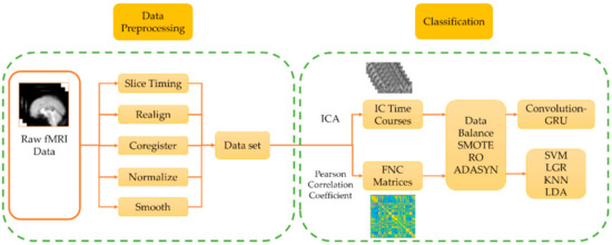
Figure 1.
The data processing framework of this study is divided into two parts: data preprocessing and classification. In the data preprocessing, the standard preprocessing process of functional magnetic resonance imaging (fMRI) is used. In data classification, independent component analysis (ICA) and Pearson correlation coefficients are performed on the processed data respectively to obtain independent component (IC) time courses and functional connectivity (FNC) matrix. After data balancing, the convolution-Gated Recurrent Unit (GRU) network and the traditional classifier are used for classification and the performance is compared.
2.3.1. Pre-Processing
In this study, SPM12 [31] is used to preprocess the data (including slice timing, realign, coregister, normalize and smooth). First slice-timing is performed to correct the time point of each brain slice, and then the realign step is performed to correct the head movement of the subject. In order to locate the points of the functional image on the anatomical image with higher resolution, the ‘coregister’ method is performed, and then, each image of the subject is normalized to the MNI standard brain space. The voxel size is resliced to 3mm × 3mm × 3mm, and image data containing 61 × 73 × 61 voxels are obtained. Finally, in order to reduce noise and improve the signal-to-noise ratio, spatial smoothing filtering is performed on the data.
After pre-processing, in order to obtain the data of each multi-target tracking task, the fMRI data of each session need to be segmented. The entire scan lasts 810 s and contains 25 MOT tasks. Although the duration of each task is 32 s, considering that there are many processes that are not related to the MOT task (such as the fixed time of 2 s at the beginning, the calculation test, etc.), It may reduce the classification effect of the classifier, so we choose 4–18 s fMRI data of each task for training. Note that the start time of the first task is the 26 th second, and the scan time of the last task is insufficient, so these two pieces of data are discarded, and finally a total of 1080 data are left for use.
2.3.2. Functional Connectivity
Functional Connectivity is a common study point in brain researches, and some past studies reported FNC to be a good tool in disease analysis [32]. In this study, the AAL90 template [33] is used to divide the preprocessed data into 90 regions. We average the time series of all voxels in each area, and use the average time series as the signal of the area. In order to obtain the correlation between the signals of each brain region, the Pearson correlation coefficient is calculated on the time series of each two brain regions:
is the mean value of the signal of region X, is the standard deviation of the signal of region X. The range of is −1 ≤ ≤ 1. When 0 < ≤ 1, it indicates that the two sets of signals have the trend to be positively correlated, and the greater the , the stronger the relationship between the two signals. When = 1, the trend of the two signals is almost the same; when −1 ≤ < 0, it means that the two signals have the trend to be negatively correlated, and the smaller the value, the stronger the negative correlation. When = −1, the trend of the signals is completely opposite. In particular, when = 0, it is generally considered that the signals are not related. After the calculation above, a 90 * 90 FNC matrix is obtained, as shown in Figure 2. Then, these FNC matrices will be input into the traditional classifier as features for classification.
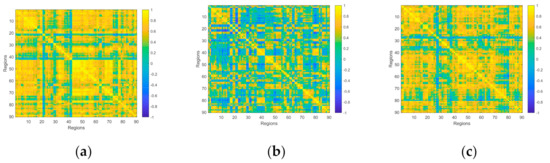
Figure 2.
The FNC matrix of three tasks performed by a subject. (a) The FNC matrix of a single target tracking task with word from word-scene pairs. (b) The FNC matrix of a multiple target tracking task with lure word. (c) The FNC matrix of a multiple target tracking task with word from word-scene pairs. It should be noted that these three pictures only represent the functional connectivity of a certain task, but not the overall situation.
2.3.3. Independent Component Analysis
Independent component analysis is a method of extracting independent features (or independent signal sources) from data. In ICA, a basic assumption is that the observed data can be viewed as a linear superposition of multiple different independent components (or signal sources). Assuming that is the observed signal, according to the previous assumption, there are independent signal sources that satisfy:
where A is a matrix of (usually full rank), and the goal of ICA is to estimate a decomposition matrix B such that:
where is the best estimate of independent signal source S.
For fMRI signals, spatial ICA is often used to extract spatial features, which can extract time-series data of non-overlapping brain regions in space. In this study, the GIG-ICA method in the group ICA toolbox [34] (GIFT, http://mialab.mrn.org/software/gift) is used to analyze the pre-processed fMRI data of all subjects. Thirty-nine independent components are obtained at first. After manually removing artifacts unrelated to the experiment and signals from unrelated brain regions, 24 spatial independent components are finally obtained (shown Figure 3), as which greatly reduced the computational cost compared to using whole brain fMRI data directly.
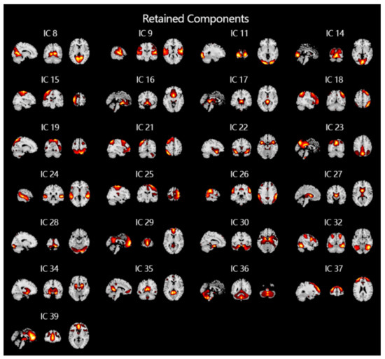
Figure 3.
The results of ICA of fMRI and removal of noise and artifacts. After performing ICA, a total of 39 independent components that do not overlap in space are obtained. After manually removing 14 noises and artifacts, the 25 independent components shown in the figure are finally obtained and used as input to the classifiers.
2.3.4. Data Oversampling
As introduced in the procedure, the MOT tasks are divided into three categories, namely: targ_easy, targ_hard, and lure_hard. In each scan, there are 10 targ_easy tasks, 10 targ_hard tasks, and 5 lure_hard tasks. Considering that the most significant difference between the three tasks is whether the word is from the word-scene pairs, so the data are divided into two categories, namely the target class and the lure class. Obviously, there is a serious imbalance in the number of samples of the two sets of data. As the majority class, the size of target class is three times that of the minority class. If the data are directly input into the classifier, it will make the classifier learn too much of the majority class data. If the data are directly input into the classifier, the test results will also be biased to the majority class, which is very disadvantageous for the training of the classifier. In order to balance the number of training samples of the two categories, this study used Synthetic Minority Oversampling Technique (SMOTE) to balance the data set.
The basic idea of the SMOTE method is to use samples from the minority class to synthesize new samples and add them to the data set, so that the number of samples is balanced. The process of SMOTE algorithm is as follows:
- First define a feature space and project all samples as points in this feature space. Then determine the sampling ratio according to the sample ratio of the majority class and the minority class.
- For each minority sample (x, y), find K samples closest to this sample according to the Euclidean distance, randomly select one (xn, yn) from the K samples, and construct a new one as follows:That is, randomly select a point on the line between the sample (x, y) and the nearest neighbor sample (xn, yn) as the new minority sample.
- Repeat the above steps until the sample size is balanced.
After processed by the SMOTE method, the number of samples of the two classes is balanced and can be used to train the classifier in the subsequent steps. It should be noted that, in order to ensure the objectivity of the experimental method, this study only performs the SMOTE method on the training set, and the test set remains unchanged.
In addition to SMOTE, there are two other data oversampling methods that are also commonly used: the random oversampling method and the adaptive synthetic (ADASYN) method. The random oversampling method is easy to implement. Its principle is to randomly sample the minority samples to increase the number of minority samples. The ADASYN method is similar to SMOTE, and its basic process is as follows:
- Calculate the degree of imbalance between the two classes:where is the sample number of the minority class and is the sample number of the majority class. When p is less than the tolerance threshold, the oversampling process begins.
- Calculate the number of samples to be synthesized:is the generation ratio, when is 1, the number of the majority class and the balanced minority class are the same.
- For each sample of the minority class, the K nearest neighbor is calculated according to the calculated Euclidean distance, and the ratio of the majority class is calculated. Obviously, .
- Standardize :
- Calculate the number of new samples that need to be generated for each minority sample:
- Generate new data in the same way as the second step of the SMOTE method until the quantity meets the requirements.
In order to test the effect of different data balancing methods on the classifier, this study also processed the training set using random oversampling and the ADASYN method, and compared the classification performances of the classifier.
2.3.5. Convolution-GRU Network
The structure of the Convolution-GRU network used in this study is shown in the Figure 4. The entire network consists of four 2-dimensional convolutional layers with convolution kernels of different sizes (3 × 6, 5 × 6, 7 × 6, 9 × 6), a LeakyReLU layer, 2 gate recurrent units (GRU), a global average pooling layer and 2 fully connected layers.
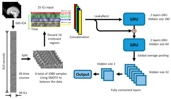
Figure 4.
The basic structure of the convolution-GRU model is to combine the spatial features obtained by convolution at four different time scales and send them to the GRU to learn the temporal features. Considering that negative values may appear in the process of convolution, the LeakyRelu layer is selected to ensure the learning of parameters. It should be noted that the number before the @ sign in this figure means the number of the channels of the convolution kernel.
First, in order to extract the spatial features in different time periods from the data (the extraction of temporal features is mainly carried out in GRU), 4 different scale convolution kernels are selected, in order to maintain the same length of the time series, padding is done in the direction of the time axis. After convolution, the data pass through the LeakyRelu layer and are concatenated together to form a 7 (TRs) * 320 (features) feature map, which will then be input into the GRU.
RNN has become one of the most commonly used time series artificial neural networks with its excellent time feature extraction ability. As a variant of LSTM network, GRU has similar performance to LSTM network, but it is easier to calculate than LSTM. In this study, two GRU models [14] with different hidden nodes connected in a feed-forward manner are used to extract high-dimensional time features from IC data. The feature map obtained in the previous step is first input into a GRU network with 180 hidden nodes, then the output of this GRU is concatenated with the previous feature map as the input of the GRU network with 64 hidden nodes.
Considering that the classifier used in this study is to classify the tasks performed by the subjects, the features of the brain activity of the subjects during the tasks are more valuable than the features at a single time point. Therefore, the output of the GRU network will go through a global average pooling layer to average the output on the entire time axis, instead of extracting only the output at the last time point to obtain a 64-dimensional feature vector. Finally, the feature vector passes through two fully connected layers to obtain the final binary classification result.
2.3.6. Statistic
In this study, we use 5 scores to evaluate the performance of the classifier; namely accuracy, majority (the large class) precision rate (LP), majority recall rate (LR), minority (the small class) precision rate (SP), and minority recall rate (SR). The calculation methods of precision rate (P) and recall rate (R) are as follows:
Among them TP, FP, TN, FN represent true positive, false positive, true negative, false negative. True and false indicate whether the classification is correct, positive and negative indicate whether the sample belongs to the positive or negative class, LP, LR, SP, SR are the results obtained when the majority class and the minority class are used as the positive class, respectively. It should be noted that the accuracy score is defined as follows:
is the number of the samples which are classified correctly by the classifier and is the number of the whole samples.
3. Results
3.1. Convolution-GRU Classification
The training and classification of the classifier in this study are completed on a laptop computer, including an Intel (R) Core (TM) i7-9750H@ 2.60GHz, 6 CPU cores and an NVIDIA GeForce GTX 1660 Ti 6.0GB GPU, and 8.0 GB memory, the classification model used are all written in Python 3.8 environment using Pytorch 1.4.0 and Sklearn 0.22.2 under Windows 10. In order to compare with the classification performance of convolution-GRU classifier, we also trained four traditional classifiers (SVM (C = 0.01), k-nearest neighbor (KNN)(n_neighbors = 2), linear discriminant analysis (LDA) (solver = ‘lsqr’), LGR) and CNN and GRU networks. It should be noted that we have used independent component data to train these classifiers, but FNC data have no time series features, so only four traditional classifiers and CNN networks have been trained. Considering that the size of the data is small, 90% of the data set is used as the training set and 10% is used as the test set to allow the classifier to learn more information, and the model is tested using 10-fold cross validation.
During the training of the convolution-GRU network, the batch size is set to 64, and we used the Adam optimizer to reduce the cross-entropy loss of the model. The initial value of the learning rate is set to 0.01, and the learning rate is adjusted using the ReduceLROnPlateau method, that is, when the decrease in three consecutive training losses is not less than a certain threshold, the learning rate is reduced to half, and the threshold is set to 0.001.
Figure 5 and Table 1 show the classification performance of seven classification methods using independent component time series as training data in this study. Classification using the convolution-GRU network resulted in a classification accuracy of 72.2 ± 2.9%, while using traditional classifiers (LDA, KNN, LGR, SVM) to classify time series of independent components yielded poor results. SVM gives the best performance in the traditional classifiers which achieved 63.2 ± 4.4%. It indicates that the convolution-GRU network used in this study has achieved a large improvement in classification accuracy. In terms of the precision and recall of the two classes, the convolution-GRU model has achieved the best classification effect of the majority class, and the precision of the minority class has also reached 26.7 ± 6%. While the precision of the majority class of the traditional classifier is comparable to that of the deep learning model, the recall of the majority class is lower, and the best performing SVM reaches only 70.9 ± 5.0%. This indicates that the convolution-GRU model has fully learned the features of the majority class. For minority class, traditional classifiers often have a higher recall rate, but the precision rate is the same or lower than some simple deep learning models, while the minority class precision rate of the convolution-GRU model reached 26.7 ± 6.1%, which shows that this model can reduce the probability that samples from majority class are misclassified, thereby improving the credibility of the classification results. For deep learning models, when CNN, GRU, or convolution-single GRU models are used for classification, the performance of the majority class is similar to the convolution-GRU model, but the performance of the minority class is poor.
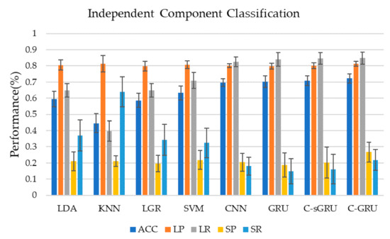
Figure 5.
Classification results using independent component time series. Convolution-GRU achieved the highest classification accuracy rate of 72.2%, while traditional classifiers performed poorly, and none exceeded 65%. Deep learning models performed similarly in the majority class, however, convolution-GRU performed best in the minority class.

Table 1.
Performance of the methods in IC classification.
Considering that LP, LR, SP, and SR have different levels in each classifier, this article uses weighted F1 values to integrate these types of index to form a comprehensive index to evaluate the classifier used in this study. In the case of imbalanced sample sizes, the weighted F1 score can objectively evaluate the performance of the classifier compared to other scores. In fact, many studies have used this indicator [35,36]. The calculation method of the weighted F1 value is as follows:
The calculated weighted F1 score of each classifier is shown in Table 2. It can be seen that under the weighted F1 score standard, the deep learning model still has great advantages over traditional classifiers. The weighted F1 value of the convolution-GRU network used in this paper reaches 0.6827, while the weighted F1 score of the KNN model is only 0.4801, which is also consistent with our previous analysis.
Table 2.
Weighted F1 of the methods in IC classification.
3.2. Comparison of Different Oversampling Strategy
In order to compare the influence of different data balancing methods on the classification performance, we used three methods, random oversampling, SMOTE, and ADASYN, to balance the training set, and trained the convolution-GRU model. The classification results are shown in Table 3. It can be seen that the accuracy of the classifier is basically consistent under the three data balancing methods. The difference between the three methods is mainly reflected in the performance of the classification of minority data. As can be seen from the table, the data processed by the SMOTE method perform significantly better than the random oversampling method and the ADASYN method in minority class, and the precision and recall rates are the highest of the three methods. This shows that the data generated by SMOTE match the distribution of the original data more than the other two commonly used data balancing methods.
Table 3.
Performance of different oversampling strategy.
3.3. Classification of Using FNC Data
In addition to the ICA of the original data, we used the AAL90 template to obtain the FNC matrix of the subjects when performing the task. In order to compare with the classification results using independent component time series data for classification, we also used the FNC matrix as input to train the classifier. It should be noted that, because the FNC matrix we calculated is static data, not time series, no model containing GRU is selected for training. As shown in Table 4 and Figure 6, when using the CNN model for classification, the highest classification accuracy rate is achieved, reaching 71.4 ± 3.6%, but the recall rate of the minority class is poor, only 11.1 ± 4.7%, very unstable. LDA and KNN in traditional classifiers perform badly. These two classifiers are too biased to divide the data into the minority class, which makes the classification performance of the majority class worse. The performance of LGR and SVM is more balanced. Although the accuracy and performance of most classes are not as good as the CNN model, they perform better in a few classes. Similarly, here also gives the weighted F1 value of each classifier when using FNC data for classification, as shown in Table 5. The deep learning model represented by CNN still maintains its advantage, reaching 0.6558, while the weighted F1 value of the KNN model is only 0.2716, which is the worst performance.
Table 4.
Performance of the methods in FNC classification.
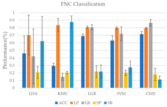
Figure 6.
Classification results using FNC matrix. Using the data of the subjects in the multi-object tracking (MOT) task to calculate the Pearson correlation coefficient to obtain the FNC matrix which is used as the input of the classifier. Since the FNC matrix itself is not a time course, so we chose CNN as the representative of the deep learning model for classification.
Table 5.
Weighted F1 of the methods in FNC classification.
In general, when using FNC as the input training classifier for classification, the three methods, LGR, SVM, and CNN, all have good performance in terms of accuracy, but the CNN method is too biased towards the learning of the majority class, resulting in the performance of the minority class is poor. The SVM and LGR methods, although the accuracy is slightly lower, the performance is relatively balanced, which shows that in the classification of FNC data, the traditional classifier represented by SVM and LGR has more advantages. In addition, if we compare Table 1 with Table 4, we will find that for traditional models, LDA and KNN methods perform poorly on both data, while LGR performs better on FNC data, and the classification performance of SVM method on the two types of data are similar. For deep learning models, since independent component time series data has temporal features in addition to spatial features, the use of convolution-GRU network can comprehensively learn two features to achieve a better classification effect than using CNN alone. Comparing Table 2 with Table 5, it can be found that in the classification task of this study, deep learning models have better classification performance, while most traditional classifiers perform poorly. On the one hand, this shows that the deep learning model is more suitable for the classification task of this study than the traditional classification model. On the other hand, it also shows that the data used in this study have a high nonlinearity and are not suitable for classification with a linear classifier.
4. Discussion
For a long time, the classification of data with a small and imbalanced sample size has been a troublesome problem, which is especially true for fMRI data. In this study, in order to solve the problem of small and imbalanced fMRI data, we proposed a three-step method. First, the ICA method is used to reduce the dimension of the data, and then the SMOTE method is used to generate the samples of the minority class to balance the number of samples. Finally, the convolution-GRU model is used and achieves an accuracy score of 72.2%. In this section, we mainly discuss the following three points: (1) The reason why the convolution-GRU method is more suitable for the fMRI data; (2) The influence of MOT task and data division on classification performance; (3) The relationship between ICA results and episodic memory studies.
In the classification of the public dataset used in this experiment, considering that too complex models may reduce the learning effect of small sample data, we used traditional classifiers such as LGR and SVM instead of CNN at first. However, as shown in the previous results, the traditional classifiers perform poorly on the fMRI data used in this study. It is because the feature dimension in this study is high and the nonlinearity is strong. SVM, LGR, LDA and other classifiers are essentially linear classifiers, which require a higher degree of linear separability of data. If they are used to classify high-dimensional nonlinear data, the effect will be reduced. Although the KNN method has no assumptions about the data and can be used for nonlinear classification, it is more sensitive to the size of the data and the degree of imbalance between the data, resulting a poor performance in classification. For these reasons, this study used ICA to reduce the dimension of the original data, and then used the SMOTE method to balance the number of two classes of samples. Finally, a convolution-GRU classifier is used to comprehensively learn the temporal and spatial features of the independent components of the data. While improving the classification performance of the majority class, the classification accuracy of the minority class is guaranteed. In addition, in this study, the FNC matrix is used as an input for classification, but since the FNC matrix does not contain temporal features, the classification performance is not as good as when independent components are used as training data.
As can be seen from the classification results, although the classification performance of the convolution-GRU classifier is better compared to traditional classifiers, the performance of the minority class is not as good as that of the majority class. On the one hand, it is due to the small sample size of the data used in this study and the high degree of non-linearity of the data. The dataset we used in this study comes from only 15 subjects, and due to the task design, the sample sizes of two classes are imbalanced. The random oversampling method only gives the random copies of the minority class, which means it cannot give more information about the class. The basic opinion of SMOTE and ADASYN is to generate new samples based on the Euclidean distance, when the data size is adequate, the two methods have enough chance to mix the samples from the minority class and generate new ones. However, for the fMRI data in this study, the lack of data makes the problem of the minority class more serious. The generated data are easier to be influenced by the noise and individual bias. We think it is an important reason why there is a high difference between the classification of the majority and minority class. On the other hand, it is also related to the task. The data used in this study come from an episodic memory experiment. Using the words from word-scene pairs to do multi-target MOT and single-target MOT tasks ten times each, and only performing multi-target MOT tasks five times for the lure words, this caused an imbalance between the two types of data. In addition, too complex tasks are also one of the reasons for the small distinction between the two task states. The difficulty of the MOT task is increased in the task, which makes the subjects pay more attention to the target tracking situation of the MOT rather than the recall of the scene when completing the task. The design of the task adopts the block design method, and there is no long resting state between different tasks. This makes the brain activation state of the subject between tasks affect each other, resulting in a smaller degree of discrimination and an increasing of the difficulty in classification. However, this does not mean that the brain state of the subjects is the same when doing two types of task. In fact, in the process of cross-validation, we have also observed several ideal classification effects. The 10-fold cross-validation used to evaluate the performance of the classifiers in this study also reflects the influence of data partitioning on the performance of the classifiers. In order to study this effect, this study further conducted 500 cross-validations on the convolution-GRU network, and obtained the classifier performance that changed with different data division conditions, as shown in the Figure 7. It can be seen that as the data division continues to change, the performance of the classifier also fluctuates. That means, there are some cases where some samples from the minority class data that are more clearly distinguished from the majority class samples are divided into the training set, making the classifier learns more unique features of the minority class and improves the classification performance.
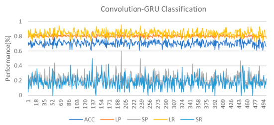
Figure 7.
The result of 500 cross-validations on the convolution-GRU network. It should be noted that we are still performing 10-fold cross-validation, so 500 cross-validation is actually 50 rounds of 10-fold cross-validation. The changes in classification performance are almost entirely derived from data division and classifier parameter initialization.
The purpose of this study is to classify the fMRI data of subjects in different task states. The biggest difference between the two categories of tasks is whether the words shown to the subjects are the words in the word-scene pairs they memorized in the previous stages. Subjects associated the given words with the scene in the pre-stage of the task and memorized this association. Obviously, the memory of the word-scene pairs constitutes a simple episodic memory. In a successful retrieval process of episodic memory, when the test word is shown, the subjects will soon be familiar with the word and remember the scene associated with the word and even the other detail of the word-scene learning session. Therefore, the classification of the fMRI data of the two tasks in this study is actually to distinguish whether the tasks performed by the subjects caused the retrieval process of episodic memory. Some past studies have shown that the recall process of episodic memory is related to the ventral parietal cortex [37,38]. There are also some studies show that the prefrontal lobe is also involved in the recall behavior of memory [39]. Compared to unsuccessful recall process, the neural activities of the “core recollection network” [40], which includes left angular gyrus, posterior cingulate cortex, medial prefrontal cortex, hippocampus, and parahippocampal cortex, are reported to be greater in successful recall process [39]. Similar results are observed in the ICA results of fMRI in this study, which shows that the task design of the word-scene pair successfully caused the recall process of the subject’s episodic memory. The ICA is proven to be a good tool to study the patterns of brain activities [15]. From past studies, we can learn the patterns indirectly by the weight of feature in classifiers, or some statistical methods, while the ICA gives us a chance to study the independent components in brain activities directly and can be combined with classification methods. However, in addition to the recall of the word-scene pairs, the MOT task is also introduced. This task is used as an interference task, which will compete with the activation of the episodic memory for visual resources and will interfere with the recall process. We think this is also the reason why the two tasks are difficult to distinguish.
In summary, this study proposes a convolutional GRU neural network based on the SMOTE method to classify small and imbalanced fMRI data from the episodic memory task with MOT, which obtained a better performance compared to traditional classifiers. At the same time, the classification results in this study also reflect whether there is a significant difference in the activation of relevant areas of the brain when the subjects perform the episodic memory task. This helps us to further understand the changes in the state of brain when people are intermittently performing the recall process of episodic memory, which has played a guiding role in the design of episodic memory-related experiments. It further reveals the operating mechanism of the memory function of the human brain under complex and diverse task environments and task conditions.
Author Contributions
Conceptualization, S.W.; methodology, S.W.; software, S.W.; validation, S.W., F.D. and M.Z.; formal analysis, S.W.; investigation, S.W. and M.Z.; resources, F.D. and M.Z.; data curation, S.W. and M.Z.; writing—original draft preparation, S.W.; writing—review and editing, S.W., F.D. and M.Z.; visualization, S.W. and M.Z.; supervision, F.D.; project administration, F.D.; funding acquisition, F.D. All authors have read and agreed to the published version of the manuscript.
Funding
This work was supported by the National Key R&D Program of China (No. 2017YFE0129700), the National Natural Science Foundation of China (No. 61673224), the Research Fellowship for International Young Scientists (No. 61850410526, 61850410524), and the Tianjin Natural Science Foundation for Distinguished Young Scholars (No. 18JCJQJC46100).
Conflicts of Interest
The authors declare no conflict of interest.
References
- Logothetis, N.K.; Pauls, J.; Augath, M.; Trinath, T.; Oeltermann, A. Neurophysiological investigation of the basis of the fMRI signal. Nature 2001, 412, 150–157. [Google Scholar] [CrossRef]
- Friston, K.J.; Holmes, A.P.; Poline, J.B.; Grasby, P.J.; Williams, S.C.; Frackowiak, R.S.; Turner, R. Analysis of fMRI time-series revisited. Neuroimage 1995, 2, 45–53. [Google Scholar] [CrossRef]
- Beckmann, C.F.; Jenkinson, M.; Smith, S.M. General multilevel linear modeling for group analysis in FMRI. Neuroimage 2003, 20, 1052–1063. [Google Scholar] [CrossRef]
- Culham, J.C.; Brandt, S.A.; Cavanagh, P.; Kanwisher, N.G.; Dale, A.M.; Tootell, R.B.H. Cortical fMRI activation produced by attentive tracking of moving targets. J. Neurophysiol. 1998, 80, 2657–2670. [Google Scholar] [CrossRef]
- Sommer, I.E.C.; Ramsey, N.F.; Kahn, R.S. Language lateralization in schizophrenia, an fMRI study. Schizophr. Res. 2001, 52, 57–67. [Google Scholar] [CrossRef]
- LaConte, S.; Strother, S.; Cherkassky, V.; Anderson, J.; Hu, X.P. Support vector machines for temporal classification of block design fMRI data. Neuroimage 2005, 26, 317–329. [Google Scholar] [CrossRef] [PubMed]
- Laconte, S.M.; Peltier, S.J.; Hu, X.P. Real-time fMRI using brain-state classification. Hum. Brain Mapp. 2007, 28, 1033–1044. [Google Scholar] [CrossRef] [PubMed]
- Savio, A.; Grana, M. Local activity features for computer aided diagnosis of schizophrenia on resting-state fMRI. Neurocomputing 2015, 164, 154–161. [Google Scholar] [CrossRef]
- Ryali, S.; Supekar, K.; Abrams, D.A.; Menon, V. Sparse logistic regression for whole-brain classification of fMRI data. Neuroimage 2010, 51, 752–764. [Google Scholar] [CrossRef] [PubMed]
- Lv, J.L.; Jiang, X.; Li, X.; Zhu, D.J.; Chen, H.B.; Zhang, T.; Zhang, S.; Hu, X.T.; Han, J.W.; Huang, H.; et al. Identifying Functional Networks via Sparse Coding of Whole Brain FMRI Signals. In Proceedings of the International IEEE/EMBS Conference on Neural Engineering, CNE, San Diego, CA, USA, 6–8 November 2013; pp. 778–781. [Google Scholar]
- Lv, J.L.; Ling, B.B.; Li, Q.Y.; Zhang, W.; Zhao, Y.; Jiang, X.; Guo, L.; Han, J.W.; Hu, X.T.; Guo, C.; et al. Task fMRI data analysis based on supervised stochastic coordinate coding. Med. Image Anal. 2017, 38, 1–16. [Google Scholar] [CrossRef]
- Jang, H.; Plis, S.M.; Calhoun, V.D.; Lee, J.H. Task-specific feature extraction and classification of fMRI volumes using a deep neural network initialized with a deep belief network: Evaluation using sensorimotor tasks. Neuroimage 2017, 145, 314–328. [Google Scholar] [CrossRef] [PubMed]
- Liu, Z.M.; de Zwart, J.A.; van Gelderen, P.; Kuo, L.W.; Duyn, J.H. Statistical feature extraction for artifact removal from concurrent fMRI-EEG recordings. Neuroimage 2012, 59, 2073–2087. [Google Scholar] [CrossRef] [PubMed]
- Yan, W.Z.; Calhoun, V.; Song, M.; Cui, Y.; Yan, H.; Liu, S.F.; Fan, L.Z.; Zuo, N.M.; Yang, Z.Y.; Xu, K.B.; et al. Discriminating schizophrenia using recurrent neural network applied on time courses of multi-site FMRI data. Ebiomedicine 2019, 47, 543–552. [Google Scholar] [CrossRef] [PubMed]
- Calhoun, V.D.; Liu, J.; Adali, T. A review of group ICA for fMRI data and ICA for joint inference of imaging, genetic, and ERP data. Neuroimage 2009, 45, S163–S172. [Google Scholar] [CrossRef]
- Dvornek, N.C.; Ventola, P.; Pelphrey, K.A.; Duncan, J.S. Identifying Autism from Resting-State fMRI Using Long Short-Term Memory Networks. Lect. Notes Comput. Sci. 2017, 10541, 362–370. [Google Scholar] [CrossRef]
- Huang, H.; Hu, X.T.; Zhao, Y.; Makkie, M.; Dong, Q.L.; Zhao, S.J.; Guo, L.; Liu, T.M. Modeling Task fMRI Data Via Deep Convolutional Autoencoder. IEEE Trans. Med. Imaging 2018, 37, 1551–1561. [Google Scholar] [CrossRef]
- Zhang, Z.W.; Duan, F.; Sole-Casals, J.; Dinares-Ferran, J.; Cichocki, A.; Yang, Z.L.; Sun, Z. A Novel Deep Learning Approach with Data Augmentation to Classify Motor Imagery Signals. IEEE Access 2019, 7, 15945–15954. [Google Scholar] [CrossRef]
- Sun, Z.; Huang, Z.H.; Duan, F.; Liu, Y. A Novel Multimodal Approach for Hybrid Brain-Computer Interface. IEEE Access 2020, 8, 89909–89918. [Google Scholar] [CrossRef]
- Suk, H.I.; Shen, D.G. Deep Learning-Based Feature Representation for AD/MCI Classification. In Proceedings of the Medical Image Computing and Computer-Assisted Intervention—MICCAI 2013, Nagoya, Japan, 22–26 September 2013; Volume 8150, pp. 583–590. [Google Scholar]
- Zhang, J.; Chen, L. Clustering-based undersampling with random over sampling examples and support vector machine for imbalanced classification of breast cancer diagnosis. Comput. Assist. Surg. 2019, 24, 62–72. [Google Scholar] [CrossRef]
- Chawla, N.V.; Bowyer, K.W.; Hall, L.O.; Kegelmeyer, W.P. SMOTE: Synthetic Minority Over-sampling Technique. J. Artif. Intell. Res. 2011, 16, 321–357. [Google Scholar] [CrossRef]
- He, H.B.; Bai, Y.; Garcia, E.A.; Li, S.T. ADASYN: Adaptive Synthetic Sampling Approach for Imbalanced Learning. In Proceedings of the IEEE International Joint Conference on Neural Networks, Hong Kong, China, 1–8 June 2008; pp. 1322–1328. [Google Scholar]
- Eslami, T.; Saeed, F. Auto-ASD-Network: A Technique Based on Deep Learning and Support Vector Machines for Diagnosing Autism Spectrum Disorder using fMRI Data. In Proceedings of the 10th ACM International Conference on Bioinformatics, Computational Biology and Health Informatics, Niagara Falls, NY, USA, 7–10 September 2019; pp. 646–651. [Google Scholar]
- Riaz, A.; Asad, M.; Alonso, E.; Slabaugh, G. Fusion of fMRI and non-imaging data for ADHD classification. Comput Med. Imag. Grap. 2018, 65, 115–128. [Google Scholar] [CrossRef] [PubMed]
- Koh, J.E.W.; Jahmunah, V.; Pham, T.H.; Oh, S.L.; Ciaccio, E.J.; Acharya, U.R.; Yeong, C.H.; Fabell, M.K.M.; Rahmat, K.; Vijayananthan, A.; et al. Automated detection of Alzheimer’s disease using bi-directional empirical model decomposition. Pattern Recognit. Lett. 2020, 135, 106–113. [Google Scholar] [CrossRef]
- Faria, F.A.; Cappabianco, F.A.; Li, C.S.R.; Ide, J.S. Information Fusion for Cocaine Dependence Recognition using fMRI. In Proceedings of the International Conference on Pattern Recognition, Cancun, Mexico, 4–8 December 2016; pp. 1107–1112. [Google Scholar]
- Poldrack, R.A.; Gorgolewski, K.J. OpenfMRI: Open sharing of task fMRI data. Neuroimage 2017, 144, 259–261. [Google Scholar] [CrossRef] [PubMed]
- Poppenk, J.; Norman, K.A. Multiple-object Tracking as a Tool for Parametrically Modulating Memory Reactivation. J. Cogn. Neurosci. 2017, 29, 1339–1354. [Google Scholar] [CrossRef]
- Cho, K.; van Merrienboer, B.; Gulcehre, C.; Bahdanau, D.; Bougares, F.; Schwenk, H.; Bengio, Y. Learning Phrase Representations using RNN Encoder-Decoder for Statistical Machine Translation. arXiv 2014, arXiv:1406.1078. [Google Scholar]
- Friston, K.J.; Holmes, A.P.; Worsley, K.J.; Poline, J.-P.; Frith, C.D.; Frackowiak, R.S.J. Statistical parametric maps in functional imaging: A general linear approach. Hum. Brain Mapp. 1994, 2, 189–210. [Google Scholar] [CrossRef]
- Duan, F.; Huang, Z.; Sun, Z.; Zhang, Y.; Zhao, Q.; Cichocki, A.; Yang, Z.; Sole-Casals, J. Topological Network Analysis of Early Alzheimer’s Disease Based on Resting-State EEG. IEEE Trans. Neural Syst. Rehabil. Eng. 2020, 28, 2164–2172. [Google Scholar] [CrossRef]
- Tzourio-Mazoyer, N.; Landeau, B.; Papathanassiou, D.; Crivello, F.; Etard, O.; Delcroix, N.; Mazoyer, B.; Joliot, M. Automated anatomical labeling of activations in SPM using a macroscopic anatomical parcellation of the MNI MRI single-subject brain. Neuroimage 2002, 15, 273–289. [Google Scholar] [CrossRef]
- Egolf, E.A.; Calhoun, V.D.; Kiehl, K.A. Group ICA of fMRI Toolbox (GIFT). Biol. Psychiatry 2004, 55, 8S. [Google Scholar]
- Zhang, X.; Kou, W.X.; Chang, E.I.C.; Gao, H.; Fan, Y.B.; Xu, Y. Sleep stage classification based on multi-level feature learning and recurrent neural networks via wearable device. Comput. Biol. Med. 2018, 103, 71–81. [Google Scholar] [CrossRef]
- Martinc, M.; Pollak, S. Combining n-grams and deep convolutional features for language variety classification. Nat. Lang. Eng. 2019, 25, 607–632. [Google Scholar] [CrossRef]
- Rugg, M.D.; King, D.R. Ventral lateral parietal cortex and episodic memory retrieval. Cortex 2018, 107, 238–250. [Google Scholar] [CrossRef] [PubMed]
- Shimamura, A.P. Episodic retrieval and the cortical binding of relational activity. Cogn. Affect. Behav. Neurosci. 2011, 11, 277–291. [Google Scholar] [CrossRef] [PubMed]
- King, D.R.; de Chastelaine, M.; Elward, R.L.; Wang, T.H.; Rugg, M.D. Recollection-Related Increases in Functional Connectivity Predict Individual Differences in Memory Accuracy. J. Neurosci. 2015, 35, 1763–1772. [Google Scholar] [CrossRef] [PubMed]
- Elward, R.L.; Vilberg, K.L.; Rugg, M.D. Motivated Memories: Effects of Reward and Recollection in the Core Recollection Network and Beyond. Cereb. Cortex 2015, 25, 3159–3166. [Google Scholar] [CrossRef]


Publisher’s Note: MDPI stays neutral with regard to jurisdictional claims in published maps and institutional affiliations. |
© 2020 by the authors. Licensee MDPI, Basel, Switzerland. This article is an open access article distributed under the terms and conditions of the Creative Commons Attribution (CC BY) license (http://creativecommons.org/licenses/by/4.0/).