Article

A Multilevel Road Alignment Model for Spatial-Query-by-Sketch

1
Key Laboratory of Virtual Geographic Environment, Nanjing Normal University, Nanjing 210023, China
2
Bremen Spatial Cognition Center, University of Bremen, 28359 Bremen, Germany
3
Jiangsu Center for Collaborative Innovation in Geographical Information Resource Development and Application, Nanjing 210023, China
4
Engineering and Computer Science Department, University Jaume I, 12071 Castellon, Spain
*
Author to whom correspondence should be addressed.
Appl. Sci. 2020, 10(21), 7685; https://doi.org/10.3390/app10217685
Submission received: 21 September 2020 / Revised: 24 October 2020 / Accepted: 26 October 2020 / Published: 30 October 2020
(This article belongs to the Section Earth Sciences)

Abstract

:
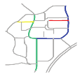
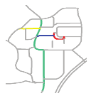
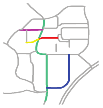
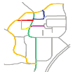
A sketch map represents an individual’s perception of a specific location. However, the information in sketch maps is often distorted and incomplete. Nevertheless, the main roads of a given location often exhibit considerable similarities between the sketch maps and metric maps. In this work, a shape-based approach was outlined to align roads in the sketch maps and metric maps. Specifically, the shapes of main roads were compared and analyzed quantitatively and qualitatively in three levels pertaining to an individual road, composite road, and road scene. An experiment was performed in which for eight out of nine maps sketched by our participants, accurate road maps could be obtained automatically taking as input the sketch and the metric map. The experimental results indicate that accurate matches can be obtained when the proposed road alignment approach Shape-based Spatial-Query-by-Sketch (SSQbS) is applied to incomplete or distorted roads present in sketch maps and even to roads with an inconsistent spatial relationship with the roads in the metric maps. Moreover, highly similar matches can be obtained for sketches involving fewer roads.

1. Introduction

With the widespread availability of the internet, people can create, publish, or query spatial data through web-based geographic information systems (GIS), such as volunteered geographic information (VGI) [1]. Geographic information systems can store, analyze, and visualize a variety of spatial information. They help for resource management, navigation, decision making, etc. Spatial query is one of the commonly used means of manipulating geographic information for individual citizens. It refers to query based on object’s name, location, distance, etc. However, existing spatial query methods for general users are usually based on single attributes, such as the feature’s name—finding a building named “Hotel”, or distance between features–finding the nearest hotel. However, if you want to find a hotel with amenities such as restaurants, shopping malls, etc. in its vicinity, a spatial combination of multiple attributes (distance, name, etc.) is required. However, existing geographic tools for common users cannot perform this query, such as Google Maps. Professional GIS tools, such as QGIS (https://qgis.org/en/site/), implement this query by first creating the hotel’s buffer, and then calculating the intersection of that buffer with the restaurants, shopping malls, etc. This process is obscure for the average users.
The key to solving this problem is whether it is possible to find ways of human-computer interaction that are close to human’s daily communication methods and can be understood by GIS systems, so that humans can communicate with computers in the same way as their counterparts [2].
A sketch map outlines a place/area/region in a drawing where the mappers represent the more characteristic elements according to their point of view. In 1948, Tolman categorized sketch maps as cognitive maps [3]. Sketch maps often reflect a strong correspondence between the spatial relations in the map and the environment and the interaction interfaces between people and their environment [4]. Individuals can create sketch maps simply by drawing an object on a paper or on a touch-sensitive screen by using a drawing software. Spatial-query-by-sketch (SQbS) [5] aligns the objects in a sketch map with those from different spatial databases. It translates a sketch map into a symbolic representation and processes it against a geographic database [6]. For example, the SketchMapia framework [7,8,9] can be used to identify seven invariant sketch features to find out a correspondence between the sketch maps and metric maps. In this framework, qualitative constraint networks based on existing qualitative calculi are compared to match the spatial objects and a new structure involving the local compatibility matrices is used to ensure partial matching and high accuracy. SQbS is a convenient tool for regular individuals owing to the following advantages: (i) individuals can conduct a spatial query without any particular background technical knowledge; (ii) in contrast to traditional query methods, which focus on a single attribute query, the approach supports scene queries; and (iii) in contrast to text queries, this approach is a more intuitive and natural query method that displays all the features. SQbS have the potential application in navigation [10], 3D shape retrieval [11], facilitating crime scene identification [12], etc.
However, according to Blaser [13], only a small quantity of objects (12–17) appears in a sketch, where human-built objects (e.g., roads and buildings) are often given more relevance than natural objects (e.g., green spaces). In addition, in Davies and Peebles [14]’s study, aspects that are visibly, semantically, or emotionally significant for them are usually given more priority, and as Meilinger et al. [15] pointed out, the aspects that mappers consider “uninteresting” are usually simplified. The incomplete, distorted, and schematized features drawn in a sketch map are also challenges for SQbS, because the data quality can significantly affect the computation results. For example, Bindzárová Gergelóvá et al. [16] found that the given hydrodynamic modeling process is sensitive to the changes of the qualitative aspect of the input data. Ślusarski and Jurkiewicz [17] developed cartographic visualization techniques to visualizing data uncertainty in the Database of Topographic Objects (DTO). In their work, three types of uncertainty (positional, attribute, and temporal) were presented using expert know-how and experiences. Hátlová and Hanus [18] reviewed 90 empirical studies published since 1960 to identify the factors which can influence the quality of the sketch map. They found that among a lot of influence factors, some overlooked factors, such as source map characteristics and geographical education, are also of importance to the quality of sketch map.
So, how to achieve the accurate alignment of the sketch map and other data sources is the focus of existing SQbS studies. Anyhow, most of the existing studies focus on the exact or constraint relaxation matching [19] of the objects’ spatial relationships. For example, Egenhofer [6] advocated SQbS based on 9-intersection model for the first time. Then Kurata and Egenhofer [20] and Kurata [21] further demonstrated 9 + -intersection relationships between directed line segments and between directed line segments and regions. Nedas et al. [22] extended the 9-intersection model by capturing metric details for line-line relations through splitting ratios and closeness measures. Lewis and Egenhofer [23] examined the topological relationships through a description of the boundary intersections between sets of objects. This approach preserved the ordering and qualitative length of these intersections. In particular, quantitative characteristics reflect individuals’ direct cognition of places and play a key role in realizing a SQbS.
Previous studies by Tang et al. [24] reported that the spatial relationships among objects, including topological, order, and location relationships, are not completely consistent between sketch maps and metric maps owing to the presence of incorrectly sketched objects or those sketched in a distorted manner. Nevertheless, main roads, as the principal routes of regional traffic, exhibit a high similarity between sketch maps and metric maps, likely because people tend to draw main roads more frequently and accurately than the rest of roads in a sketch map. This aspect can be attributed to the fact that roads and paths connect places and are frequently used for navigation. This finding is consistent with the visual judgement of individuals, specifically, two places are deemed to be similar not only because they have similar spatial relationships but also because they have similar structural characteristics, such as shapes. The roads produced by the participants in the study by Tang et al. [24] were drawn at a planning conceptualization level according to Timpf et al. [25]. The instructional or driver road conceptualizations did not appear maybe because participants were not asked to draw roads, but a place, so detail about road lanes, exits, or entrances was missing. The main goal of this paper is to enhance the correspondence between sketch maps and metric maps. For that, a novel matching approach termed Shape-based Spatial-Query-by-Sketch (SSQbS) is presented, which is based on a SQbS taking into account the road shape. A three-level road alignment model including individual roads, composite roads, and road scenes is developed. This approach is suitable for application to incomplete or distorted roads along with roads with an inconsistent topological relationship matching between the sketched maps and the metric maps.
The remaining paper is structured as follows. Section 2 provides a review of the related work. Section 3 presents the sketched road characteristics in the three considered levels and describes how the main roads are extracted from a sketch. In addition, the descriptors and matching approaches for individual roads, composite roads, and road scenes are also explained in this section, respectively. Section 4 describes the conducted experiment and presents and discusses the matching results. The conclusions and scope for future work are presented in Section 5.

2. Related Work

Shape-based query-by-sketch techniques have been widely used for image retrieval. Gottfried [26] asserted that the shape of a sketched object is useful to identify other images containing similarly shaped objects by considering their spatial structures. For that, Gottfried [27,28,29] proposed a global feature scheme based on a qualitative representation in which tripartite line tracks were used to describe polygons and bipartite arrangements were used to describe the relation between two disconnected objects. Bai et al. [30] applied the discrete curve evolution (DCE, [31]) to decompose complete contours and created the MPEG-7 (Moving Picture Experts Group) database of contour segments. Their representation of object parts was invariant to scaling, rotation, and translation; moreover, smaller misalignments in the contours have a robust shape context that allows shape matching. Falomir et al. [32] presented a Qualitative Shape Descriptor (QSD) to describe the contour of an object shape extracted from any digital image and also a computational approach to compare the QSDs obtained in order to identify shape correspondences. Cao et al. [33] built the multimodal MindFinder system, which can retrieve sketches from millions of images. Their system allowed users to outline the main shapes by tagging and colouring. Xiao et al. [34] improved the MindFinder framework using a shape word descriptors for sketch-based image retrieval and they employed the classical Chamfer Matching Algorithm by [35] to address the shape word matching problems. Furthermore, Xiao et al. [34] proposed the use of an inverted index structure to extend the shape word expression to a wide range of image databases.
In addition, shape-based road alignment has been applied for vector road network matching. Zhang [36] adopted a turning function as the descriptor of the road shapes. Touya et al. [37] proposed a framework based on the least squares adjustment [38,39] and position constraints to match object geographic shapes. Tong et al. [40] formulated a logistic regression matching method named OILRM (Optimization and Iterative Logistic Regression Matching), which is used to determine the distance between two lines based on their vertices for road matching. Kim et al. [41] compared the angles and directions of linear features and obtained high accuracy results by further comparing the topological relationships between the matched features. To carry out shape comparison in images, Ali Abbaspour et al. [42] studied three functions (turning, signature, and tangent functions) and three shape descriptors (shape context, LORD, and shape signature). In addition, Ali Abbaspour et al. [42] demonstrated that the turning function can be used to efficiently distinguish objects in terms of their shapes. In particular, the existing studies on shape-based query-by-sketch for image retrieval [26,27,28,29,30,31,33,34] focused on a small number of objects for comparison, whereas a sketch map may contain typically 12–17 objects [13]. Furthermore, the spatial relationships among objects also must be aligned to carry out Spatial-Query-by-Sketch. In the approach presented in this paper, the main roads from sketch maps are extracted, because they have been demonstrated to exhibit considerable similarities between sketch maps and metric maps [24]. In addition, the characteristics of the main roads are further analyzed and compared quantitatively and qualitatively at three levels: individual road, composite road, and road scene. Consequently, the approach presented here is different from those reported by Zhang [36] and Tong et al. [40], in which only quantitative characteristics (e.g., turning functions or distances between vortices) were adopted for road matching. The proposed approach differs from the work by Kim et al. [41] as we surveyed more than one spatial relationship (topological relationship). Moreover, owing to the particularity of sketch maps, the approach presented in this paper varies from the traditional vector road data query (e.g., Touya et al. [37], Ali Abbaspour et al. [42]) as it overcomes the following aspects: (1) inaccuracy of drawn objects: in sketch maps, roads are often distorted, partially drawn, or missing local details; (2) omitted objects: the number of objects in a sketch map is often not the same as that in a metric map because people tend to sketch only the objects that are meaningful to them; and (3) the inaccurate representation of spatial relationships (e.g., distance and orientation): for example, a sketch can qualitatively indicate that one road is longer than another road; however, the quantitative distance between the two roads may not be accurately described.

3. Materials and Methods

A multilevel road model is proposed for road alignment in Section 3.1. Based on this multilevel road model, the characteristics of individual road (Section 3.2), composite road (Section 3.3), and road scene (Section 3.4) are described and compared between the sketch map and the metric map, respectively.

3.1. Multilevel Road Classification

The multilevel road model employed in the approach presented in this paper includes three levels: individual road, composite road, and road scene.
  • A individual road refers to a road in a given location. For example, R0’, R1’, R2’, and R3’ are individual roads in the road network shown in Figure 1a.
  • A composite road contains two individual and intersected roads. For example, the yellow line composed of R0’ and R1’ is a composite road in the road network shown in Figure 1a.
  • A road scene represents the combination of all the roads in a given location. The green line composed of R0’, R1’, R2’, and R3’ in Figure 1a represents a road scene.
First, the individual roads are extracted from a sketch map. Then, roads in sketch maps are aligned with those in a metric map progressively in three levels. In the first level, individual roads are compared between the sketch maps and the metric map, based on three characteristics: shape distance, number of critical turning points, and circulation direction. Next, according to the matching results of the individual roads and considering the first matching priority, composite roads from the sketch maps and metric map are matched in terms of the topological relationship among their characteristics, order of appearance along one intersection, and relative positions of the intersections. In the third level, road scene matching is performed with respect to (w.r.t.) the road with the second matching priority, characteristics’ frequency for a matched road, intersection order along the road, and topological relation between the roads without matching priorities. The details are presented in the following subsections.
The framework used for sketched road matching is illustrated in Figure 2.

3.2. Characteristics and Matching Approach for Individual Roads

In this section, the descriptors that represent a individual road are introduced. Furthermore, the approach of matching individual roads between a sketch map and a metric map is presented. The extraction of main roads from the sketch map is described in Section 3.2.1. To represent a individual road, the following three features are adopted: (i) shape distance, which indicates the distance between two roads in terms of the shape (Section 3.2.2); (ii) number of critical turning points, which describes the curvature of individual roads (Section 3.2.3); and (iii) circulation direction, which indicates the direction of two adjacent road segments (Section 3.2.4). The calculation for individual road matching is described in Section 3.2.5.

3.2.1. Extraction of Main Roads

Main roads are the principal routes for regional traffic. According to analysis by Tang et al. [24], main roads exhibit a high similarity between a sketch map and a metric map. The proposed approach attempts to extract the main roads from sketch maps and match them with the roads shown in a metric map. The method reported by Jiang and Claramunt [43] is considered, which is an expansion of the approach proposed by Freeman [44] to classify streets in an urban street network using three factors:
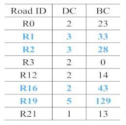
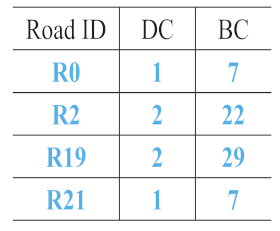
  • The degree centrality ( D C ), also known as the connectivity, indicates the number of roads connected to a certain road. A given road is considered more important if a larger number of roads are connected to it. In Figure 1a, R2’ has three roads connected to it (R0’, R1’, and R3’); therefore, the D C of R2’ is 3. R3’ has only one road (R2’) connected to it, and therefore, the corresponding D C is 1. Consequently, R2’ is more important than R3’ in terms of D C .
  • The betweenness centrality ( B C ) is a measure of the frequency at which a certain road is passed in all the shortest paths of a given location. A higher frequency indicates a greater connectivity of a road. In the proposed approach, B C is determined by calculating the shortest path from one endpoint of a certain road to the endpoints of all the other roads and considering the occurrence frequency of a road in all the shortest paths as the B C in that road in a given location. According to Figure 1b, the occurrence frequencies for each road that appeared in all the shortest paths are 4 (R0’), 4 (R1’), 6 (R2’), and 4 (R3’). This demonstrates that R2’ is more important than the other roads in this location, in terms of the B C .
  • The closeness centrality ( C C ), in graph theory, is based on the degree to which a point is close to all the other points. In terms of roads, the C C indicates the shortest distance from a given road to all the other roads. Because the objective of this study is to determine the main roads in a given location, this factor is not calculated when extracting the main roads.
Specifically, the proposed approach adopts the D C and B C to extract the main roads from a sketch map. Roads with higher values of D C and B C can be considered as the main roads in a location. For example, according to the above analysis, R2’ is a main road in the considered location, as it corresponds to the highest D C and B C values.
Figure 3 shows a road from a sketch (represented by R0) and the corresponding road from OpenStreetMap (OSM, OpenStreetMap: https://www.openstreetmap.org/). Note that, OSM is a map of the world, and the roads in it are models of real-world roads.
Certain roads extracted from OSM (represented by R1, R2, R3, R4, and R5 in Figure 4) were extracted for further calculation and comparison, as discussed in the subsequent sections.

3.2.2. Shape Distance

The shape distance ( S D ) describes the shape difference between two roads. The approach proposed by Vatavu et al. [45] was adopted, in which unordered points are used to represent the stroke shape, and the stroke number, order, and direction are ignored. To match two point clouds, an approximation of the Hungarian algorithm [46] is used to obtain the aligned points. Subsequently, the Euclidean distance between each aligned point is computed, and the sum of the distances is considered as the dissimilarity between the two points. Based on this method, in the proposed approach, the dissimilarity is calculated as the S D between two roads, as shown in Formula (1):
S D ( S k e t c h , O S M ) =   d i s ( R S k e t c h , R O S M )
where S D ( S k e t c h , O S M ) represents the S D between two roads, R S k e t c h represents a road from a sketch; R O S M represents a road from OSM, and d i s ( R S k e t c h , R O S M ) represents the dissimilarity of the roads from the sketch map and OSM, based on the approach of Vatavu et al. [45]. When comparing two roads, a smaller value of S D indicates that the shapes of two roads are more similar. Table 1 lists the S D between R0 and R1–R5. Of the five roads (R1–R5), R3 and R4 are the most similar to R0 because they have smaller S D (4.21 and 4.74). In addition, R3 and R4 in Figure 4 have higher visual similarities to R0 in Figure 3a.

3.2.3. Number of Critical Turning Points

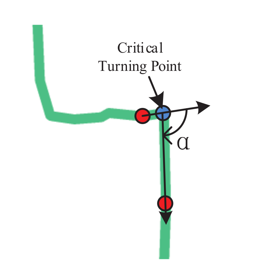
The number of critical turning points ( N C T P ) outlines the structure of a road. A critical turning point is a point at which the direction difference (represented by α in Figure 5) between two neighboring line segments is greater than a certain threshold, as represented by the blue circle in Figure 5. The threshold is based on the features of the road itself, and the minimum value of all the large corner points along a road line is typically selected as the threshold.
It is reasonable to consider that two roads are likely to be similar only when the N C T P of one road from OSM is equal to or exceeds that of a road from a sketch, as shown by Formula (2):
S i m N C T P ( S k e t c h , O S M ) N C T P O S M N C T P S k e t c h ? T r u e : F a l s e
where S i m N C T P ( S k e t c h , O S M ) ) represents the similarity in terms of the N C T P between two roads; N C T P O S M and N C T P S k e t c h respectively represent the N C T P of a road from OSM and that of a road from a sketch. Table 2 shows the N C T P for R0–R5, considering a threshold of 36 . It can be observed that R3–R5 (which can be visually observed to be more similar to the sketched road) have N C T P values that are equal to or more than those of R0.

3.2.4. Circulation Direction

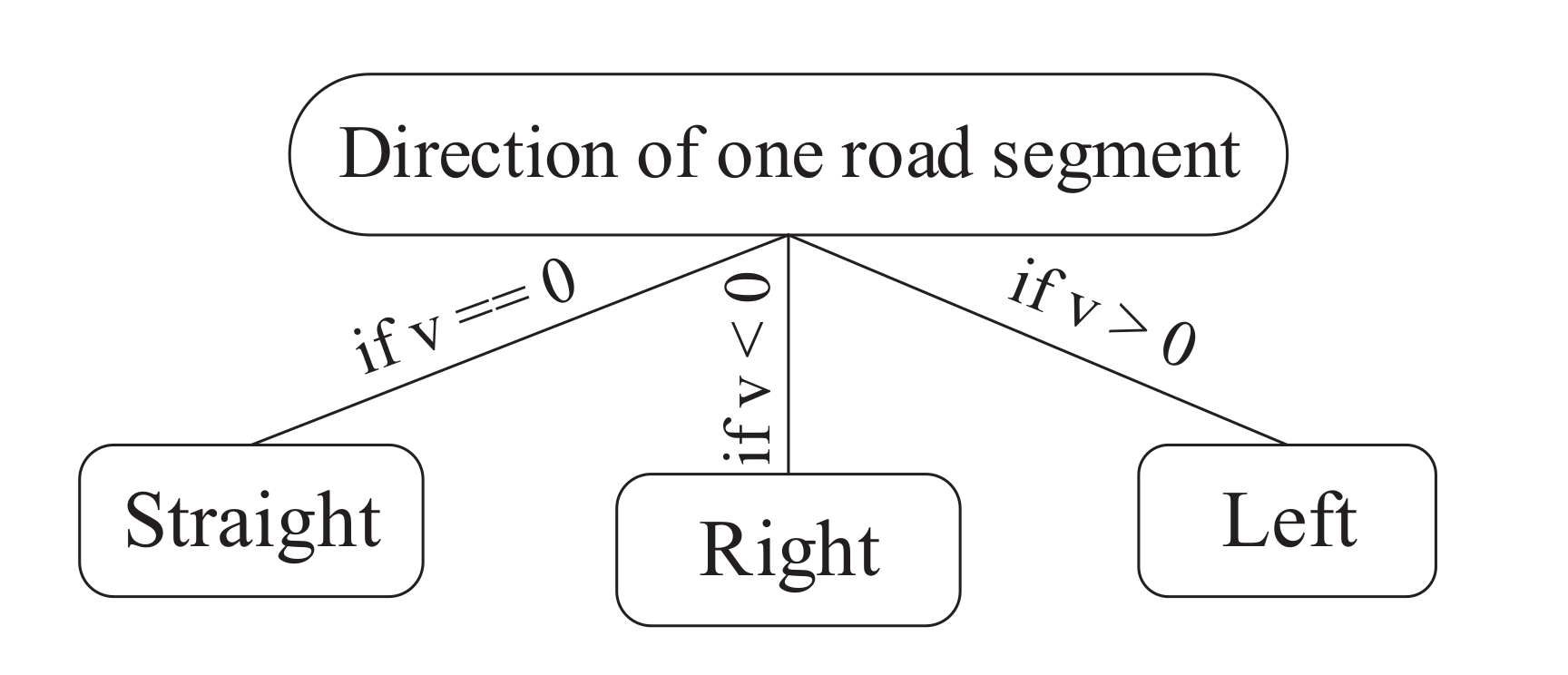
The circulation direction [29] of a individual road ( C D ) identifies the direction of each road segment w.r.t. to its previous road segment. The proposed approach firstly computes the direction difference for two adjacent road segments with Formula (3) and then obtains the circulation direction of one road segment as depicted in Figure 6.
v = ( x p 0 x p 1 ) ( y p 1 y p 2 ) ( x p 1 x p 2 ) ( y p 0 y p 1 )
where p 0 represents the start vertex of the first road segment; p 1 is the end vertex of the first segment and also the start vertex of next road segment; p 2 is the end point of the next road segment.
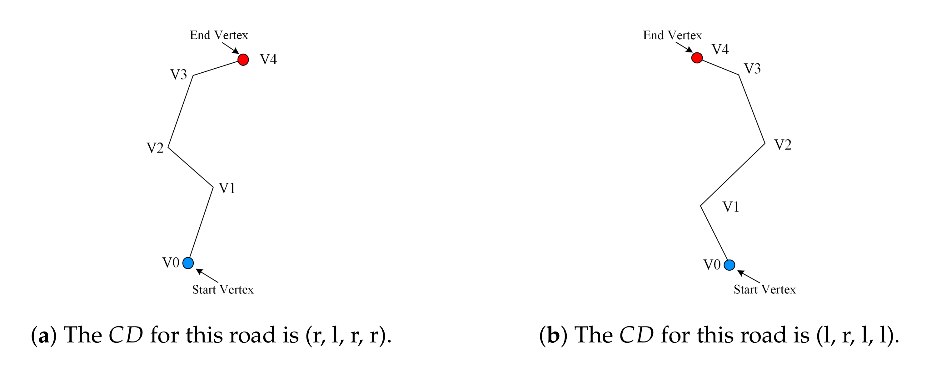
The left and right directions for each road segment are represented as “l” and “r”, respectively. Figure 7 shows the C D of two roads. The road in Figure 7a turns right, then left, then right, and finally right again. The road in Figure 7b turns left, then right, then left, and finally left again.
If the C D of one road is the same as that of another road, the two roads are considered to be similar in terms of the C D . If the C D of one road is part of that of another road, the two roads are considered to be partially similar. Formula (4) shows the computation of similarity in terms of the C D .
S i m C D ( S k e t c h , O S M ) C D S k e t c h C D O S M ? T r u e : F a l s e
where S i m C D ( S k e t c h , O S M ) represents the similarity between two roads in terms of the C D ; C D S k e t c h and C D O S M represent the C D of a road from a sketch and that of a road from OSM, respectively. Table 3 presents the C D of R0 and R1–R5. The C D of R1 is null, as it is a straight road. The C D of R0 is the same as that of R3 and R4. Moreover, the C D of R0 is part of that of R5, which means that R0 is partially similar to R5. These findings are consistent with those of a visual inspection.

3.2.5. Computation of Similarity between Individual Roads

The similarity between two individual roads is the sum of the similarities w.r.t. the shape distance ( S D ), number of critical turning points ( N C T P ), and circulation direction ( C D ) described in the above sections. Formula (5) can be used to compute the similarity between two roads:
S i m R = w 1 · ( S a m p l e N U M S D ) + w 2 · S i m N C T P + w 3 · S i m C D
where S i m R represents the similarity between two individual roads. S a m p l e N U M is the number of sampling points involved in the S D computation, which was assigned a value of 32 in the approach by Vatavu et al. [45]. w 1 , w 2 , and w 3 respectively represent the weight assigned to the similarity in terms of the S D , N C T P , and C D . It holds that w 1 + w 2 + w 3 = 1.0 . S i m N C T P and S i m C D respectively represent the similarity between two roads in terms of the N C T P and C D . Furthermore, a larger value of S i m R indicates a higher similarity between two roads. In this work, as all the features in Formula (5) have the same importance, the weights are assigned the same value: 1 3 . These weights may be tuned according to different research needs.

3.3. Characteristics and Matching Approach for Composite Roads

A composite road is formed by two individual and intersected roads. The characteristics of a composite road include: (i) the first matching priority (Section 3.3.1); (ii) the topological relationship between the roads (Section 3.3.2); (iii) the order of appearance along an intersection (Section 3.3.3); and (iv) the relative intersection positions in the roads (Section 3.3.4). The approach to compute the similarity between composite roads is described in Section 3.3.5.

3.3.1. First Matching Priority

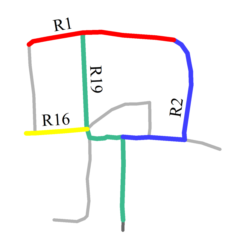
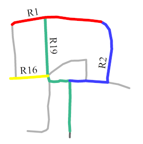
The first matching priority ( F M P ) refers to the priority of a individual road during the process of matching a composite road. The accuracy of the matching results obtained by different individual roads differs owing to the particularities of individual roads. The F M P is thus adopted to narrow the search range and increase the matching accuracy. The F M P can be assigned to an individual road that has a higher shape specificity and a higher degree centrality. For example, in Figure 8, R2 and R19 are more curved than R1 and R16; therefore, the F M P will be assigned to R2 or R19. Furthermore, the degree centrality of R19 is 5 and that of R2 is 3, so F M P can be assigned to R19.

3.3.2. Topological Relationship of Composite Roads

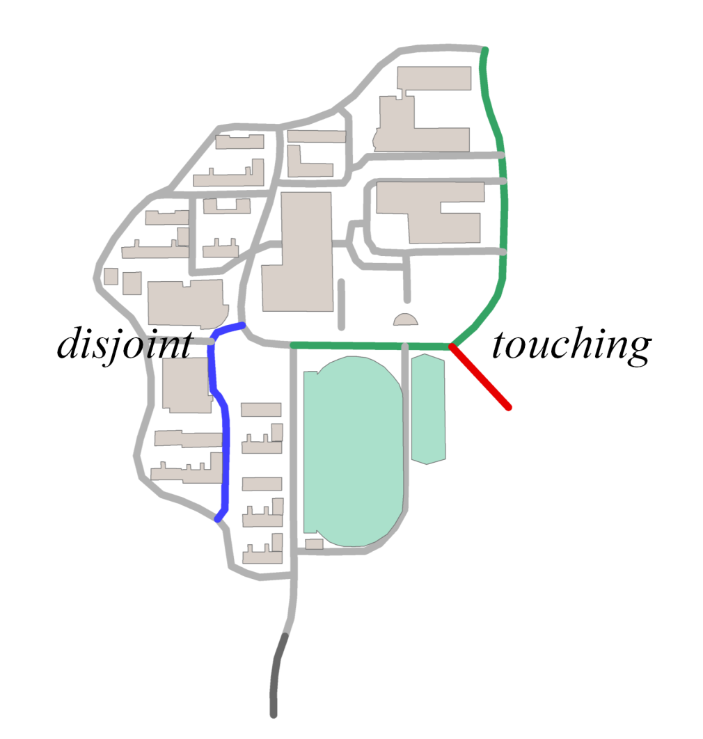
The topological Relationship ( T R ) characterizes the connection between two individual roads. According to analysis by Tang et al. [24], the topological relationships of main roads are highly similar between sketch maps and the metric map. The 9-intersection model reported by Egenhofer and Herring [47] is adopted to describe the topological relationship between roads. This model uses a 3 × 3 intersection matrix to describe the relationship between two features in the inner part (I), boundary (B), and external part (E). Figure 9 shows an example of two topological relationships, namely, touching and disjoint. Open source lib geos (geos: https://github.com/libgeos/geos/) is adopted to compute the topological relationship between two vector roads.
If the topological relationships between the two roads that constitute a composite road are the same between the sketch map and metric map, the two composite roads are considered to be similar in terms of the T R . Formula (6) can be used to calculate the similarity in terms of the T R between two roads:
S i m T P ( S k e t c h , O S M ) T P O S M T P S k e t c h ? T r u e : F a l s e
where S i m T P ( S k e t c h , O S M ) represents the similarity in T R between two composite roads derived from a sketch and OSM; T P S k e t c h represents the T R of the composite road from a sketch; and T P O S M represents the T R of the composite road from OSM.

3.3.3. Order of Appearance of Roads along an Intersection

The order of appearance of connected roads along an intersection ( O D ), as defined by Herring [48], describes the orientation relationship between connected roads.
As shown in Figure 10, the proposed approach first computes the buffer (represented by Buffer) of a certain radius at the intersection (represented by P) of two roads.
In this case, the order of appearances of the connected roads along P are represented by the x-coordinate values (represented by x 1 , x 2 , and x 3 ) of the intersections (represented by p 1 , p 2 , and p 3 ) between the roads and Buffer. In Figure 10, the O D along P is R S k e t c h 2 , R S k e t c h 1 , and R S k e t c h 1 , because the corresponding x-coordinate values of the intersections between Buffer and the roads are x 1 , x 2 , and x 3 , respectively.
If the orders of appearance along an intersection are the same between the roads from the sketch and those from OSM, the roads are considered to be similar in terms of the O D , as shown in Formula (7):
S i m O D ( S k e t c h , O S M ) O D O S M O D S k e t c h ? T r u e : F a l s e
where S i m O D ( S k e t c h , O S M ) represents the similarity between two composite roads from a sketch and OSM, in terms of the O D ; O D O S M represents the O D of one composite road from the sketch; and O D S k e t c h represents the O D of one composite road from OSM.

3.3.4. Relative Positions of Intersections

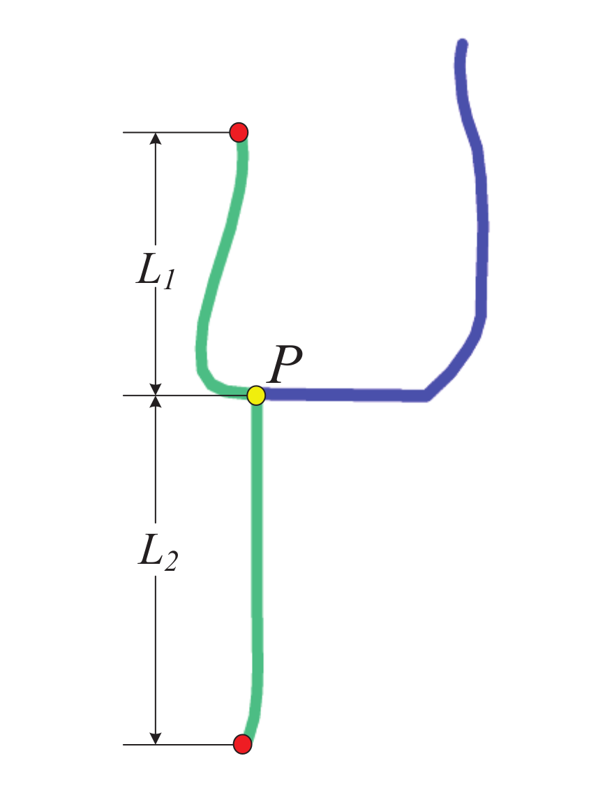
The relative positions of the intersections ( R P I ) in two connected roads can further clarify the connection between two roads. As shown in Figure 11, P is the intersection of two connected roads (green and blue lines). L 1 and L 2 refer to the lengths of two parts of the road (in green) separated at P.
The similarity between two roads in terms of the R P I can be determined using the following process:
  • The lengths of two parts of a road separated by P are computed for both the sketch and OSM aspects to obtain L 1 OSM , L 2 OSM , L 1 Sketch , and L 2 Sketch ;
  • The absolute distances Δ d OSM and Δ d Sketch are computed using Formulas (8) and (9):
    Δ d O S M =   L 1 O S M L 2 O S M
    Δ d S k e t c h =   L 1 S k e t c h L 2 S k e t c h
  • Δ d OSM and Δ d Sketch are normalized on the basis of the length of the roads in OSM and sketches to obtain Nor OSM and Nor Sketch (see Formulas (10) and (11)), respectively:
    N o r O S M = Δ d O S M / L O S M
    N o r S k e t c h = Δ d S k e t c h / L S k e t c h
  • The distance D Nor between Nor OSM and Nor Sketch is compared to obtain S i m P I ( S k e t c h , O S M ) in terms of the R P I . If D Nor is smaller than or equal to T h r e s h o l d P I , the composite roads from a sketch and OSM are considered similar, as expressed in (12) and (13):
    D N o r =   N o r O S M N o r S k e t c h
    S i m R P I ( S k e t c h , O S M ) D N o r T h r e s h o l d P I ? T r u e : F a l s e
    where S i m R P I ( S k e t c h , O S M ) represents the similarity between two composite roads from the sketch and OSM, in terms of the R P I , and T h r e s h o l d P I is the threshold defined to compare the similarity in terms of the R P I .

3.3.5. Computation of Similarity between Composite Roads

The similarity between two composite roads is the sum of the similarities in terms of topological relationship ( T R ), order of appearance of connected roads along one intersection ( O D ) and relative positions of intersections ( R P I ) depicted in the above sections. Formula (14) can be used to compute the similarity between composite roads from OSM and a sketch.
S i m C R = w 4 · S i m R 1 + w 5 · S i m R 2 + w 6 · S i m T P + w 7 · S i m O D + w 8 · S i m R P I
where S i m C R represents the similarity between two composite roads. S i m R 1 and S i m R 2 denote the similarities between two individual roads that constitute the composite road. w 4 and w 5 denote the weights assigned to S i m R 1 and S i m R 2 , respectively. S i m T P , S i m O D , and S i m R P I respectively represent the similarity between two composite roads in terms of the T R , O D , and R P I . w 6 , w 7 , and w 8 respectively represent the weights assigned to S i m T P , S i m O D , and S i m R P I . It holds that w 4 + w 5 + w 6 + w 7 + w 8 = 1.0 . A larger S i m C R corresponds to a higher similarity between two composite roads. As all the features in Formula (14) have the same relevance, the weights are assigned the same value 1 5 . In other works, these weights may be tuned differently.

3.4. Characteristics and Matching Approach for Road Scenes

A road scene consists of all the roads in a given location. The characteristics of a road scene include:(i) the second matching priority (Section 3.4.1); (ii) the frequency of a matched individual road appearing in all the resulting composite road matches (Section 3.4.2); (iii) intersections ordered along a individual road with priority (Section 3.4.3); and (iv) the topological relationship between roads without matching priorities (Section 3.4.4). The computation of the road scene similarity is described in Section 3.4.5.

3.4.1. Second Matching Priority

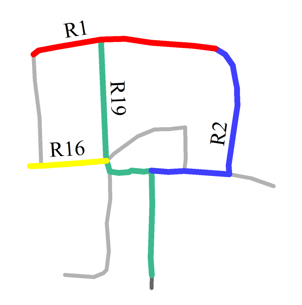
The second matching priority ( S M P ) is adopted to assign a matching priority to the second road that forms the composite road with the road that has the first matching priority ( F M P , see Section 3.3.1), to reduce the matching range. For example, in Figure 12, R19 and R2 are more curved than R1 and R16; therefore, S M P can be assigned to R2 if F M P is assigned to R19. Scene matching is performed on the basis of a composite road with F M P and S M P .

3.4.2. Frequency of a Matched Road

The frequency of a matched road ( F M R ) represents the frequency of a matched individual road that appears in all the resulting composite road matches. If a individual road from OSM appears in the composite road matches with a higher frequency, it is more likely that the road scene including this road is similar to the road scene from the sketch. For example, in Figure 13, R156137559 appears in all the composite road matches: “Sketch R19 Touches R2”, “Sketch R19 Touches R1”, and “Sketch R19 Touches R16”. It can be inferred that the road scene that includes R156137559 in OSM is more similar to that including R19 in the sketch.

3.4.3. Intersection Order of Roads along One Main Road

The intersections order ( I O ) represents the orientation relationship of other roads along the road with the first matching priority. If the I O along the road with the first matching priority ( F M P , see Section 3.3.1) is consistent between two road scene, the two road scenes are considered to be similar in terms of the I O . If the I O of a road scene is part of that of another road scene, the two road scene are considered to be partially similar.
First, the intersections between all the other roads and the road with F M P are determined. Then, all the other roads are sorted according to the coordinate values of these intersections. For example, in Figure 14a, I O along road R19 is {R1, R16, R2}. In Figure 14b, I O along road R19 is {R1, R16, R2, R1}. Because {R1, R16, R2} is part of {R1, R16, R2, R1}, it can be inferred that I O along R19 in Figure 14a is part of I O along R19 in Figure 14b; therefore, the two road scenes are considered to be partially in similar terms of the I O .
The similarity of two road scenes in terms of the I O can be computed as follows.
S i m I O ( S k e t c h , O S M ) I O S k e t c h I O O S M ? T r u e : F a l s e
where S i m I O ( S k e t c h , O S M ) represents the similarity in I O between two road scenes from a sketch and OSM; I O S k e t c h represents the I O of a road scene from a sketch; and I O O S M represents the I O of a road scene from OSM.

3.4.4. Topological Relationship between Roads without Matching Priorities

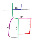
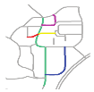
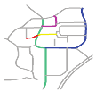
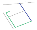
The topological relationship between roads without matching priorities ( T R M P ) describes the spatial relationship between roads without matching priorities and can further distinguish the similarity between road scenes in terms of the topological relationships. For example, in Figure 15, the green road is a road assigned with matching priority, and the yellow and blue roads are roads without matching priorities. The T R M P between the yellow and blue roads in Figure 15b (touching) is the same as that between the yellow and blue roads in Figure 15a (touching) and different from that between the yellow and blue roads in Figure 15c (disjoint). The similarity between two road scenes in terms of the T R M P can be computed as follows:
S i m T R M P ( S k e t c h , O S M ) T R M P S k e t c h T R M P O S M ? T r u e : F a l s e
where S i m T R M P ( S k e t c h , O S M ) represents the similarity in T R M P between two road scenes from a sketch and OSM; T R M P S k e t c h represents the T R M P of a road scene from a sketch; and T R M P O S M represents the T R M P of a road scene from OSM.

3.4.5. Computation of Similarity between Road Scenes

The similarity of two road scenes is the sum of the similarities in each composite road that constitute the road scene, intersection order ( I O ) and topological relationship between roads without matching priorities ( T R M P ) detailed in above sections. The similarity between two road scenes can be obtained as follows:
S i m S R = w 9 · i n S i m C R i + w 10 · S i m I O + w 11 · S i m T R M P
where S i m S R represents the similarity between two road scenes; S i m C R i represents the similarity of the i-th composite road that constitutes the road scene; and n is the number of composite roads that constitute the road scene. w 9 is the weight assigned to the sum of all S i m C R i . S i m I O and S i m T R M P respectively represent the similarity of two road scenes in terms of the I O and T R M P . w 10 and w 11 respectively represent the weight assigned to S i m I O and S i m T R M P . It holds that w 9 + w 10 + w 11 = 1.0 . A larger S i m S R corresponds to more similar road scenes. In our paper, the weights in Formula (17) have been all assigned the same value ( 1 3 ) since all the features have the same relevance. Other studies may turn these weights differently.

4. Results and Discussion

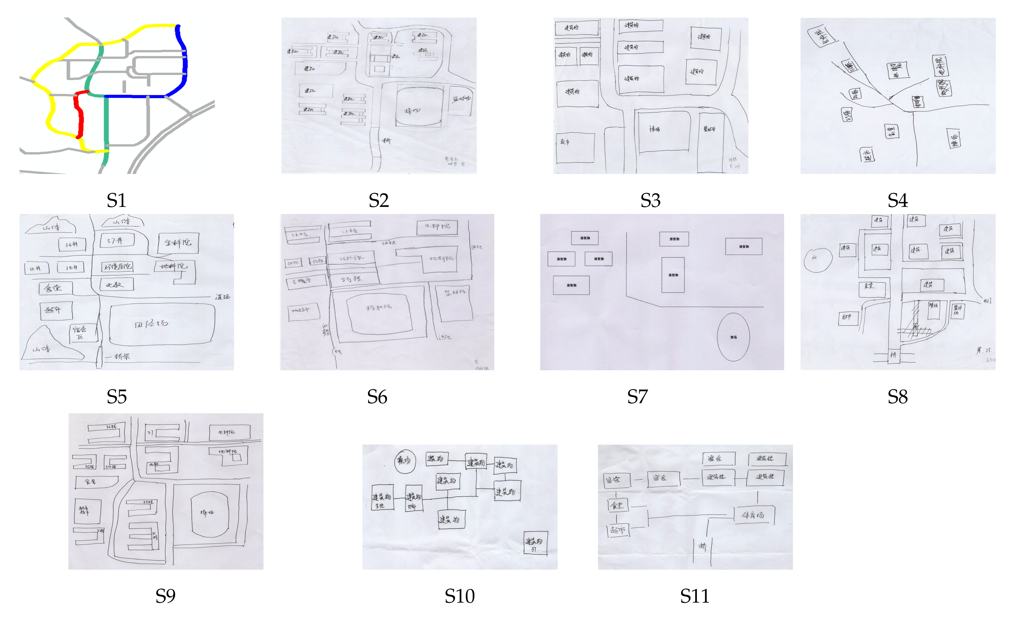
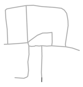
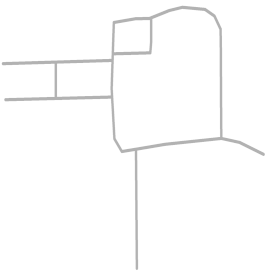
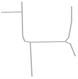
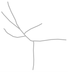
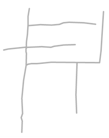
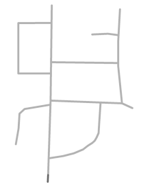
We invited participants to draw a sketch of the northern campus of the Xianlin University District of Nanjing Normal University, Nanjing, China (see https://www.openstreetmap.org/relation/9356340\#map=17/32.11603/118.91191), as shown in Figure 16. Eleven participants (four male and seven female participants) with ages ranging from 20 to 30 years sketched the same experimental area. Nine participants had geographical knowledge as their major was in the GIS domain, whereas two participants had no geographical background but had used Google Maps before. Figure 17 shows the sketches, numbered S1–S11, drawn by the 11 participants. OpenStreetMap (OSM) data was taken as the reference data for alignment. The sketches were digitized manually to build the road network. Main roads in each sketch were extracted and adopted for the test application. The approach described above was used to do matching experiments between each sketch and OSM data, as discussed in Section 4.2.

4.1. Extracting Main Roads

All these sketch maps refer to the same place, but their similarity is low. This might be due to the fact that each participant reflected his/her particular understanding of the place [49]. Therefore, it was necessary to extract the main roads from the sketch maps. It should be noted that certain sketched roads such as those appearing in sketches S10 and S11 are schematic and do not reflect the shapes of the roads. These schematic roads only represent the accessibility or connection between two places/buildings. Therefore, the roads in these sketches were not included in our subsequent road-related matching calculations.
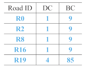
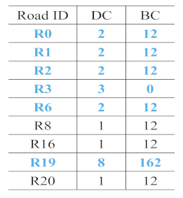
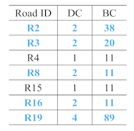
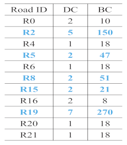
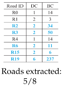
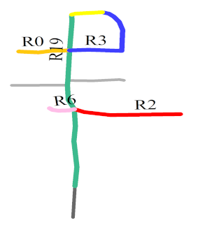
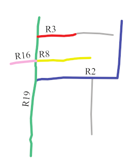
The parameters of degree centrality ( D C ) and betweenness centrality ( B C ) were adopted, as described in Section 3.2.1, to extract the main roads from the sketches. Roads with high values of both D C and B C were considered as the main roads. Figure 16d presents all the roads in the experimental area, as extracted from OSM, and the main roads, which are central roads in the experiment area. Table 4 shows all the roads drawn in each sketch except sketch S7, and the main roads extracted from each sketch according to their D C and B C . Only two roads were drawn in sketch S7, so both of them were extracted as main roads.
From Table 4, the following observations could be made:
  • R2 and R19 were most frequently extracted as the main roads. These roads are consistent with the main roads in OSM, as shown in Figure 16d. The same ID was assigned to the same roads in each sketch to facilitate the analysis.
  • The number of main roads extracted from each sketch was different, as shown in the lower part of the second column in Table 4. The maximum number was 6 (S5), and the minimum number was 2 (S7); however, almost half the roads in each sketch were extracted as the main roads.
  • In sketches S3, S4, and S7, all the roads were extracted as the main roads. In S3, the D C and B C values were the same for R2 and R19 and for R0 and R21. In S4, all the roads except for R19 had the same D C and B C . In S7, only two roads were drawn.
  • In S5, R0, R1, R2, R3, R6, and R19 were selected as the main roads as they had the same values of D C and B C . In S9, although R1, R2, R3, R6, and R15 had similar D C values, R1 was not chosen as a main road owing to its lower B C . This aspect also holds for R0 and R16 in S8.

4.2. Road Scene Matching

After extracting the main roads from each sketch, as shown in Table 4, matching experiments were performed between each sketch and OSM to compute the road similarities. The experiments included three steps: individual road matching, composite road matching, and road scene matching. A shapefile containing 15,242 roads of Nanjing, China, from OSM was used as a matching database. The computation time was between 58.2 s and 1803 s. Table 5 presents the matching results from this database.
  • Each row in Table 5 shows the main roads extracted from each sketch, the matching parameters, and the matching results from OSM.
  • The first column in Table 5 lists the IDs of the sketches, corresponding to those in Figure 17.
  • The second column lists the main roads extracted from the sketches. In addition, the matching parameters are listed, including MaxMN, which represents the maximum number of roads from OSM involved in the matching of the road from one sketch with the first matching priority ( F M P , see Section 3.3.1), and ThresholdCon, which represents the threshold of the direction difference for comparing the circulation direction ( C D , see Section 3.2.4) values.
  • The remaining columns show the top-ranked matching results from the database based on the main roads extracted from each sketch. The similarity between each road scene from OSM and that from each sketch is also presented. The greater the similarity, the more similar are the roads between the sketch and OSM.
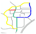
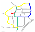
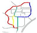
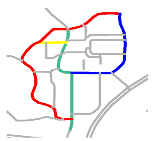
Formula (17) was used to align roads between the sketch map and the metric map. A value of 100 was adopted to quantitatively compute the similarity if the similarity between two roads in Formulas (2)–(4), (6), (7), (13), (15) and (16) was True. In contrast, a value of 0 was used if the similarity between two roads in these formulas was False. The weights involved in in Formulas (5), (14) and (17) were averaged: the values of w 1 , w 2 , and w 3 in Formula (5) were set to 0.33 ; the values of w 4 , w 5 , w 6 , w 7 , and w 8 in Formula (14) were set to 0.2 ; and the values of w 9 , w 10 , and w 11 in Formula (17) were set to 0.33.
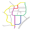
Furthermore, it should be noted that two different matching results are shown for S5 in Table 5, as the topological relationships of the red and green roads are varied between OSM (disjoint) and S5 (touching). The matching results of the first row for S5 corresponds to the top three results obtained without considering the topological relationship of these two roads. The matching results for the second row for S5 correspond to the top three results obtained considering the topological relationship of these two roads.
Figure 18 shows the whole time cost of each sketch in roads matching. It can be found that:
  • matching of sketch S9 costs the shortest time, because the quantity of main roads extracted in sketch S9 is the least (3), and also two main sketched roads in scene S9 are curved. Note that there are only two sketched roads in sketch S7, so the time cost for matching of sketch S7 is just used for composite road matching.
  • matching of sketch S6 costs the longest time. As it can be seen from Table 4, sketch S6 has only one curved main road, and the remaining main roads in sketch S6 are all nearly straight. Moreover, there were five roads extracted as main roads in sketch S6 for matching, which correspondingly increased the matching time.

4.3. Discussion

As indicated in Table 5, all the sketch maps could be used to query the accurate corresponding roads from OSM, except for S7. The key experimental results are as follows.
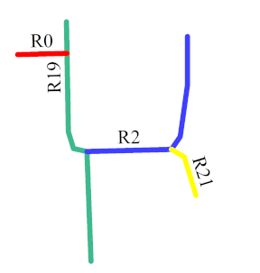
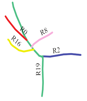
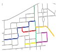
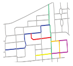
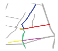
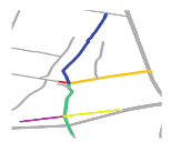
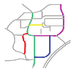
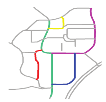
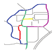
Although the roads were drawn partially or distorted in several sketch maps, accurate matching results could be obtained, including those for sketches S1, S2, S4–S6, S8, and S9. In Table 5, S1 has one partially drawn road (red line), but an accurate metric road map was observed in the top matching result. This finding also holds for S2, S4, S5, and S9 (having a partially drawn road in red, blue, green, and purple, respectively). Furthermore, the accurate matching results of these sketch maps were in the top three results.
Accurate matching results could also be obtained for sketch maps with distorted roads. For example, in S4, all the main roads were drawn in a distorted manner except for the one in blue; nevertheless, the exact match was in the second place (see Table 5). S6 (distorted road in green) and S8 (distorted road in purple) also exhibited accurate matching results in the third and first places, respectively.
Accurate matching results could be obtained for sketch maps involving inconsistent topological relationships between roads with those in the metric map. In S5, two roads (in red and blue) were drawn inconsistently with those in the metric map, which led to an inconsistent topological relationship see Figure 19. Thus, two rows of matching results were shown for sketch S5, in which one row shows the matching results obtained considering the topological relationship between these two roads, while the other row shows the results obtained not considering this relationship (see the two rows of matching results for S5 in Table 5). Nevertheless, an accurate matching result ( S i m S R = 201.744) was obtained, even when the topological relationship between the two roads was not considered (see the first row of matching results for S5 in Table 5).
Accurate road maps could not be obtained for S7 from OSM, as shown in Table 5. This can be attributed to the small number of roads (only 2) drawn in the sketch and the fewer curves of these roads (see Table 4).
In particular, the characteristic first matching priority ( F M P , see Section 3.3.1) can be assigned to a road with more shape curves and a higher degree centrality value in one sketch map. More curved shape can improve the similarity in computing shape distance. A higher degree centrality value means more roads connected to this road as we discussed in Section 4.1 and correspondingly involves more composite roads matchings. For example, in sketch S1, green road is more curved than other main roads extracted. Furthermore, its degree centrality value (3) is the highest as Table 5 shows. This holds for the same road in sketches S2–S7 and S9. Whereas in sketch S8, the same road (in purple) is a straight line, so F M P was assigned to the road in green. Characteristic F M P can help narrow the search range, as demonstrated in Section 3.3.1.

5. Conclusions and Future Work

This paper proposes a shape-based approach for spatial-query-by-sketch, known as Shaped-based Spatial-Query-by-Sketch. In the work by Tang et al. [24], it was noted that main roads exhibit considerable similarities between the sketch maps and the metric map. Considering this aspect, in this work, the data for main roads were obtained from sketch maps based on two factors, namely, the degree centrality and betweenness centrality. Subsequently, the main roads were compared in three levels quantitatively and qualitatively—individual road, composite road, and road scene. In the first level, we calculated the similarities between two individual roads considering quantitative characteristics, such as the shape distance, and qualitative characteristics such as the circulation direction. In the second level, the topological relationship and quantitative characteristics of a composite road (i.e., composed of two individual roads), such as the relative positions of the intersections, were aligned between the sketch maps and the metric map. In the third level, all the main roads extracted from a sketch map were further quantitatively and qualitatively compared with those in the metric map based on the road scene characteristics, e.g., the frequency of a matched road. Next, the matching results were sorted based on the sum of the characteristic similarities. An experiment was performed, in which nine sketch maps drawn by nine participants were aligned with the metric map derived from OSM. The results indicated that for eight out of nine sketch maps, accurate road maps could be obtained from the metric map. The inaccurate matching of the remaining sketch map was a result of the small number of roads in the sketch (only 2) and the presence of only a few shape curves in the roads. Furthermore, it was noted that accurate matching results could be obtained for sketch maps with partially drawn roads or distorted roads and even for roads with an inconsistent topological relationship with those in the metric map.
The following aspects are expected to be a part of future work:
  • Comparison of the spatial relationship between roads and buildings, such as the orientation relationship, topological relationship, and ordering relationship. In particular, in some sketches, only a few roads are drawn, which makes it challenging to match these roads. Combining the sketched roads with buildings may improve the accuracy of matching.
  • Development of a method to match the sketched places with discrete sketched roads. Discrete sketched roads are road segments generated during the process of digitization. Specifically, in this work, the roads in the sketch maps were digitized manually and the road integrity was guaranteed. In future work, the digitization will be conducted automatically, by decomposing the roads in the sketch maps into several line segments. Note that the shape of a discrete sketched road may be different from that of a completely sketched road, and the topological relationship between such roads may also be different. Therefore, in future work, we intend to realize matching between discrete sketched roads and complete roads in the metric map.
  • Application of the proposed model to an unknown experimental area. In this study, the road similarity was examined considering roads in familiar places. An objective of future work is to study the characteristics and consistency of roads in unfamiliar scenes.

Author Contributions

Conceptualization, M.T., Z.F., and Y.S.; methodology, M.T. and Z.F.; software, M.T.; validation, M.T.; formal analysis, M.T.; investigation, M.T. and Z.F.; resources, M.T.; data curation, M.T.; writing—original draft preparation, M.T.; writing—review and editing, Z.F. and Y.S.; visualization, M.T.; supervision, Z.F. and Y.S.; project administration, Z.F. and Y.S.; funding acquisition, Y.S. All authors have read and agreed to the published version of the manuscript.

Funding

This research was funded by the Key Fund of National Natural Science Foundation of China (grant number 41631175), the National Key Research and Development Program of China (grant number 2017YFB0503500).

Acknowledgments

Part of this work was carried out while M.T. was a doctoral research fellow at the Bremen Spatial Cognition Center. Z.F. acknowledges funding by the Cognitive Qualitative Descriptions and Applications (CogQDA) project at the University of Bremen and also the Ramon y Cajal fellowship (RYC2019-027177-I/AEI/10.13039/501100011033) awarded by the Spanish Ministry of Science, Innovation and Universities. We particularly thank all those who participated in our experiment, as well as our colleagues who provided helpful and significant comments.

Conflicts of Interest

The authors declare no conflict of interest.

Abbreviations

The following abbreviations are used in this manuscript:
VGIVolunteer Geographic Information
GISGeographic Information System
SQbSSpatial-Query-by-Sketch
SSQbSShape-based Spatial-Query-by-Sketch
DCEDiscrete Curve Evolution
QSDQualitative Shape Description
DCDegree Centrality
BCBetweenness Centrality
CCCloseness Centrality
OSMOpenStreetMap
SDShape Distance
NCTPNumber of Critical Turning Points
CDCirculation Direction
FMPFirst Matching Priority
TRTopological Relationship
ODOrder of Appearance of connected roads along one intersection
RPIRelative Positions of Intersections
SMPSecond Matching Priority
FMRFrequency of a Matched Road
IOIntersection Order
TRMPTopological Relationship between roads without Matching Priorities

References

  1. Goodchild, M.F. Citizens as sensors: The world of volunteered geography. GeoJournal 2007, 69, 211–221. [Google Scholar] [CrossRef] [Green Version]
  2. Guo, D. Geospatial Analysis Based on Spatial Scene Similarity; China Science Publishing & Media Ltd. (CSPM): Beijing, China, 2016. [Google Scholar]
  3. Tolman, E.C. Cognitive maps in rats and men. Psychol. Rev. 1948, 55, 189. [Google Scholar] [CrossRef] [PubMed] [Green Version]
  4. Freksa, C.; Moratz, R.; Barkowsky, T. Schematic maps for robot navigation. In Spatial Cognition II; Springer: Berlin/Heidelberg, Germany, 2000; pp. 100–114. [Google Scholar] [CrossRef]
  5. Egenhofer, M.J. Spatial-query-by-sketch. In Proceedings of the 1996 IEEE Symposium on Visual Languages, Boulder, CO, USA, 3–6 September 1996; pp. 60–67. [Google Scholar] [CrossRef]
  6. Egenhofer, M.J. Query processing in spatial-query-by-sketch. J. Vis. Lang. Comput. 1997, 8, 403–424. [Google Scholar] [CrossRef] [Green Version]
  7. Schwering, A.; Wang, J.; Chipofya, M.; Jan, S.; Li, R.; Broelemann, K. SketchMapia: Qualitative representations for the alignment of sketch and metric maps. Spat. Cogn. Comput. 2014, 14, 220–254. [Google Scholar] [CrossRef] [Green Version]
  8. Chipofya, M.C.; Schultz, C.; Schwering, A. A metaheuristic approach for efficient and effective sketch-to-metric map alignment. Int. J. Geogr. Inf. Sci. 2016, 30, 405–425. [Google Scholar] [CrossRef]
  9. Jan, S.; Schwering, A.; Schultz, C.; Chipofya, M. Cognitively plausible representations for the alignment of sketch and geo-referenced maps. J. Spat. Inf. Sci. 2017, 2017, 31–59. [Google Scholar] [CrossRef]
  10. Jia Wang, R.L. An Empirical Study on Pertinent Aspects of Sketch Maps for Navigation. Int. J. Cogn. Inform. Nat. Intell. 2013, 7, 26–43. [Google Scholar] [CrossRef]
  11. Wang, F.; Kang, L.; Li, Y. Sketch-based 3D shape retrieval using convolutional neural networks. In Proceedings of the IEEE Conference on Computer Vision and Pattern Recognition, Boston, MA, USA, 7–12 June 2015; pp. 1875–1883. [Google Scholar] [CrossRef]
  12. Dutelle, A.W. An Introduction to Crime Scene Investigation; Jones and Bartlett Learning: Burlington, MA, USA, 2016. [Google Scholar]
  13. Blaser, A.D. Sketching Spatial Queries. Ph.D. Thesis, Spatial Information Science and Engineering, University of Maine, Orono, ME, USA, 2000. [Google Scholar]
  14. Davies, C.; Peebles, D. Spaces or scenes: Map-based orientation in urban environments. Spat. Cogn. Comput. 2010, 10, 135–156. [Google Scholar] [CrossRef]
  15. Meilinger, T.; Riecke, B.E.; Bülthoff, H.H. Local and global reference frames for environmental spaces. Q. J. Exp. Psychol. 2014, 67, 542–569. [Google Scholar] [CrossRef]
  16. Gergelóvá, M.B.; Kuzevičová, Ž.; Labant, S.; Gašinec, J.; Kuzevič, Š.; Unucka, J.; Liptai, P. Evaluation of Selected Sub-Elements of Spatial Data Quality on 3D Flood Event Modeling: Case Study of Prešov City. Appl. Sci. 2020, 10, 820. [Google Scholar] [CrossRef] [Green Version]
  17. Ślusarski, M.; Jurkiewicz, M. Visualisation of Spatial Data Uncertainty. A Case Study of a Database of Topographic Objects. Int. J. Geo-Inf. 2020, 9, 16. [Google Scholar] [CrossRef] [Green Version]
  18. Hátlová, K.; Hanus, M. A Systematic Review into Factors Influencing Sketch Map Quality. Int. J. Geo-Inf. 2020, 9, 271. [Google Scholar] [CrossRef]
  19. Nedas, K.A.; Egenhofer, M.J. Spatial-scene similarity queries. Trans. GIS 2008, 12, 661–681. [Google Scholar] [CrossRef]
  20. Kurata, Y.; Egenhofer, M.J. The head-body-tail intersection for spatial relations between directed line segments. In International Conference on Geographic Information Science; Springer: Berlin/Heidelberg, Germany, 2006; pp. 269–286. [Google Scholar] [CrossRef]
  21. Kurata, Y. The 9+-intersection: A universal framework for modeling topological relations. In International Conference on Geographic Information Science; Springer: Berlin/Heidelberg, Germany, 2008; pp. 181–198. [Google Scholar] [CrossRef] [Green Version]
  22. Nedas, K.A.; Egenhofer, M.J.; Wilmsen, D. Metric details of topological line-line relations. Int. J. Geogr. Inf. Sci. 2007, 21, 21–48. [Google Scholar] [CrossRef]
  23. Lewis, J.A.; Egenhofer, M.J. Oriented regions for linearly conceptualized features. In International Conference on Geographic Information Science; Springer: Cham, Switzerland, 2014; pp. 333–348. [Google Scholar] [CrossRef]
  24. Tang, M.; Falomir, Z.; Freksa, C.; Sheng, Y.; Lyu, H. Extracting invariant characteristics of sketch maps: Towards Place Query-by-Sketch. Trans. GIS 2020, 24, 903–943. [Google Scholar] [CrossRef]
  25. Timpf, S.; Volta, G.; Pollock, D.; Frank, A.; Egenhofer, M. A Conceptual Model of Wayfinding Using Multiple Levels of Abstraction. In Theories and Methods of Spatio-Temporal Reasoning in Geographic Space; Lecture Notes in Computer Science; Springer: Berlin/Heidelberg, Germany, 1992; Volume 639. [Google Scholar] [CrossRef] [Green Version]
  26. Gottfried, B. Shape from Positional-Contrast: Characterising Sketches with Qualitative Line Arrangements; Deutscher Universitäts-Verlag: Wiesbaden, Germany, 2007. [Google Scholar] [CrossRef]
  27. Gottfried, B. Global Feature Schemes for Qualitative Shape Descriptions. In IJCAI-05 Workshop Notes on Spatial and Temporal Reasoning; 2005; Available online: https://citeseerx.ist.psu.edu/viewdoc/download?doi=10.1.1.73.634&rep=rep1&type=pdf (accessed on 26 October 2020).
  28. Gottfried, B. Querying for silhouettes by qualitative feature schemes. In Proceedings of the 2nd International Conference on Document Image Analysis for Libraries (DIAL’06), Lyon, France, 27–28 April 2006; pp. 281–290. [Google Scholar] [CrossRef]
  29. Gottfried, B. Qualitative similarity measures-the case of two-dimensional outlines. Comput. Vis. Image Underst. 2008, 110, 117–133. [Google Scholar] [CrossRef]
  30. Bai, X.; Yang, X.; Latecki, L.J. Detection and recognition of contour parts based on shape similarity. Pattern Recognit. 2008, 41, 2189–2199. [Google Scholar] [CrossRef] [Green Version]
  31. Latecki, L.J.; Lakämper, R. Convexity rule for shape decomposition based on discrete contour evolution. Comput. Vis. Image Underst. 1999, 73, 441–454. [Google Scholar] [CrossRef] [Green Version]
  32. Falomir, Z.; Gonzalez-Abril, L.; Museros, L.; Ortega, J.A. Measures of similarity between objects based on qualitative shape descriptions. Spat. Cogn. Comput. 2013, 13, 181–218. [Google Scholar] [CrossRef] [Green Version]
  33. Cao, Y.; Wang, H.; Wang, C.; Li, Z.; Zhang, L.; Zhang, L. Mindfinder: Interactive sketch-based image search on millions of images. In Proceedings of the 18th ACM International Conference on Multimedia, Firenze, Italy, 25–29 October 2010; ACM: New York, NY, USA, 2010; pp. 1605–1608. [Google Scholar] [CrossRef]
  34. Xiao, C.; Wang, C.; Zhang, L.; Zhang, L. Sketch-based image retrieval via shape words. In Proceedings of the 5th ACM on International Conference on Multimedia Retrieval, Shanghai, China, 23–26 June 2015; ACM: New York, NY, USA, 2015; pp. 571–574. [Google Scholar] [CrossRef]
  35. Borgefors, G. Hierarchical chamfer matching: A parametric edge matching algorithm. IEEE Trans. Pattern Anal. Mach. Intell. 1988, 10, 849–865. [Google Scholar] [CrossRef]
  36. Zhang, M. Methods and Implementations of Road-Network Matching. Ph.D. Thesis, Technische Universität München, Munich, Germany, 2009. [Google Scholar]
  37. Touya, G.; Coupé, A.; Jollec, J.L.; Dorie, O.; Fuchs, F. Conflation optimized by least squares to maintain geographic shapes. ISPRS Int. J. Geo-Inf. 2013, 2, 621–644. [Google Scholar] [CrossRef]
  38. Harrie, L.E. The constraint method for solving spatial conflicts in cartographic generalization. Cartogr. Geogr. Inf. Sci. 1999, 26, 55–69. [Google Scholar] [CrossRef]
  39. Sester, M. Optimization approaches for generalization and data abstraction. Int. J. Geogr. Inf. Sci. 2005, 19, 871–897. [Google Scholar] [CrossRef]
  40. Tong, X.; Liang, D.; Jin, Y. A linear road object matching method for conflation based on optimization and logistic regression. Int. J. Geogr. Inf. Sci. 2014, 28, 824–846. [Google Scholar] [CrossRef]
  41. Kim, I.H.; Feng, C.C.; Wang, Y.C. A simplified linear feature matching method using decision tree analysis, weighted linear directional mean, and topological relationships. Int. J. Geogr. Inf. Sci. 2017, 31, 1042–1060. [Google Scholar] [CrossRef]
  42. Ali Abbaspour, R.; Chehreghan, A.; Karimi, A. Assessing the efficiency of shape-based functions and descriptors in multi-scale matching of linear objects. Geocarto Int. 2018, 33, 879–892. [Google Scholar] [CrossRef]
  43. Jiang, B.; Claramunt, C. A structural approach to the model generalization of an urban street network. GeoInformatica 2004, 8, 157–171. [Google Scholar] [CrossRef]
  44. Freeman, L.C. Centrality in social networks conceptual clarification. Soc. Netw. 1978, 1, 215–239. [Google Scholar] [CrossRef] [Green Version]
  45. Vatavu, R.D.; Anthony, L.; Wobbrock, J.O. Gestures as point clouds: A $P recognizer for user interface prototypes. In Proceedings of the 14th ACM international conference on Multimodal interaction, Santa Monica, CA, USA, 22–26 October 2012; ACM: New York, NY, USA, 2012; pp. 273–280. [Google Scholar] [CrossRef]
  46. Kuhn, H.W. The Hungarian method for the assignment problem. Nav. Res. Logist. Q. 1955, 2, 83–97. [Google Scholar] [CrossRef] [Green Version]
  47. Egenhofer, M.J.; Herring, J.R. Categorizing Binary Topological Relations between Regions, Lines, and Points in Geographic Databases; Technical Report; Department of Surveying Engineering, University of Maine: Orono, ME, USA, 1990. [Google Scholar]
  48. Herring, J. The mathematical modeling of spatial and non-spatial information in geographic information systems. In Cognitive and Linguistic Aspects of Geographic Space; Springer: Dordrecht, The Netherlands, 1991; pp. 313–350. [Google Scholar] [CrossRef]
  49. Eden, C. On the nature of cognitive maps. J. Manag. Stud. 1992, 29, 261–265. [Google Scholar] [CrossRef]
Figure 1. Representation of a road scene and its corresponding connectivity matrix. (a) A road scene showing four individual roads (black line segments: R0’, R1’, R2’, and R3’); one composite road (yellow line: R0’ and R1’); and five individual road endpoints (blue circles) and their IDs (black and blue colors correspond to roads and endpoints, respectively). (b) Connectivity matrix of the road network shown in Figure 1a.
Applsci 10 07685 g001
Figure 2. Framework for sketched road matching.
Applsci 10 07685 g002
Figure 3. A road from a sketch and the corresponding road from OSM.
Applsci 10 07685 g003
Figure 4. Individual roads extracted from OSM.
Applsci 10 07685 g004
Figure 5. Direction difference (represented by α ) of two neighboring road segments. The blue circle represents a critical turning point; the two red circles represent two adjacent points of the critical turning point.
Applsci 10 07685 g005
Figure 6. Direction of one road segment. Note that, v is the difference value in direction of two adjacent road segments obtained in Formula (3).
Applsci 10 07685 g006
Figure 7. C D of two roads. Note that V0–V4 represent the vertices of the roads. V0 and V4 respectively represent the starting and end vertices of the road.
Applsci 10 07685 g007
Figure 8. Main roads (in color) with different curves.
Applsci 10 07685 g008
Figure 9. Topological relationships between roads. T R between the green and red roads corresponds to the touching facet. T R between the blue road and the two other roads (green and red) corresponds to a disjoint relationship.
Applsci 10 07685 g009
Figure 10. P is the intersection of two roads R S k e t c h 1 and R S k e t c h 2 . Buffer is the buffer of a certain radius at P. Points p 1 , p 2 , and p 3 indicate the intersections between Buffer and the two roads. x 1 , x 2 , x 2 are the x-coordinate values of points p 1 , p 2 , and p 3 , respectively.
Applsci 10 07685 g010
Figure 11. P (yellow circle) is the intersection of two roads (green and blue). L 1 and L 2 denote the lengths of two parts of one road (green) separated at P.
Applsci 10 07685 g011
Figure 12. Roads (in color) with different curves.
Applsci 10 07685 g012
Figure 13. R156137559 appears in all the composite road matches. The first level of each tree view in the resulting composite road matches represents each composite road from the sketch. The child nodes represent the matched composite roads from OSM sorted according to the roads’ similarities to the parent composite road from the sketch.
Applsci 10 07685 g013
Figure 14. Roads R1, R2, and R16 (red, yellow, and blue lines, respectively) intersect with road R19 (green line) at I1, I2, I3, and I4, respectively.
Applsci 10 07685 g014
Figure 15. Road scene from the sketch (left), and two road scenes from OSM (middle and right). The topological relationship between the roads with T R M P in Figure 15a is the same as that in Figure 15b and different from that in Figure 15c. (a) Road scene from a sketch. The green road has matching priority. The topological relationship between the yellow and blue roads is that of touching. (b) Candidate road scene from OSM. The topological relationship between the yellow and blue roads is that of touching. (c) Another candidate road scene from OSM. The topological relationship between the yellow and blue roads is disjoint.
Applsci 10 07685 g015
Figure 16. Experiment area and the roads in the experiment area. (a) Northern campus of Xianlin University District of Nanjing Normal University (taken by Da-Jiang unmanned aerial vehicle Phantom 4). (b) Metric map of the experiment area in Chinese (from OSM© OpenStreetMap) contributors. (c) Metric map of the experiment area in English (from OSM© OpenStreetMap contributors). The annotations in (c) are the English explanations of corresponding objects’ annotations in (b). (d) Roads from OSM. The numbers represent the road IDs. The green and blue roads are two main roads.
Applsci 10 07685 g016
Figure 17. Sketches drawn by participants. Note that, the Chinese annotations in the sketches are the categories or names of the objects labeled by volunteers. S10 and S11 were not included in the subsequent analysis because the sketched roads in these two sketches were schematic and did not reflect the road shapes.
Applsci 10 07685 g017
Figure 18. Time cost for roads matching in each sketch.
Applsci 10 07685 g018
Figure 19. Different topological relationships of the corresponding two roads in OSM and S5.
Applsci 10 07685 g019
Table 1. S D between R0 and R1–R5. Note that 4.21 and 4.74 are in bold because R3 and R4 have the smaller SD w.r.t. R0.
Road IDR1R2R3R4R5
S D btw the sketched
road (R0) and roads from OSM
6.947.584.214.745.00
Table 2. N C T P of R0 and R1–R5. (The threshold of the direction difference is 36 ).
Road from a SketchRoads from OSM
Road IDR0R1R2R3R4R5
N C T P 201243
S i m N C T P ( Sketch , OSM ) -NoNoYesYesYes
Table 3. C D of R0 and R1–R5.
A Road
in a Sketch
Roads from OSM
Road IDR0R1R2R3R4R5
C D l, r-rl,rl,rr,l,r
S i m C D ( S k e t c h , O S M ) -NoNoYesYesYes
Table 4. Main roads extracted from each sketch w.r.t. D C and B C . Note that roads in sketch S7 were all extracted as main roads, because there are only two roads in the sketch.
Roads in
each sketch
Applsci 10 07685 i001
S1
Applsci 10 07685 i002
S2
Applsci 10 07685 i003
S3
Applsci 10 07685 i004
S4
Applsci 10 07685 i005
S5
Applsci 10 07685 i006
S6
Applsci 10 07685 i007
S8
Applsci 10 07685 i008
S9
DC and BC Applsci 10 07685 i009
Roads extracted:
4/10
Applsci 10 07685 i010
Roads extracted:
4/8
Applsci 10 07685 i011
Roads extracted:
4/4
Applsci 10 07685 i012
Roads extracted:
5/5
Applsci 10 07685 i013
Roads extracted:
6/9
Applsci 10 07685 i014
Roads extracted:
5/7
Applsci 10 07685 i015
Roads extracted:
5/10
Applsci 10 07685 i016
Roads extracted:
5/8
Main roads
(in color)
Extracted
Applsci 10 07685 i017 Applsci 10 07685 i018 Applsci 10 07685 i019 Applsci 10 07685 i020 Applsci 10 07685 i021 Applsci 10 07685 i022 Applsci 10 07685 i023 Applsci 10 07685 i024
Table 5. Matching results for all sketches. F M P is assigned to the green road. MaxMN is the maximum number of matched individual roads from OSM involved in the process of composite road matching. ThresholdCon is the threshold of the direction difference for computing C D of the green road.
Sketch IDMain Roads Extracted
and Matching Parameters
Top Three Matching Results from the Roads of Nanjing,
China, in OSM and Their Similarities
S1 Applsci 10 07685 i025
MaxMN = 30
ThresholdCon = 36
Applsci 10 07685 i026
146.899
Applsci 10 07685 i027
145.066
Applsci 10 07685 i028
144.987
S2 Applsci 10 07685 i029
MaxMN = 30
ThresholdCon = 36
Applsci 10 07685 i030
141.254
Applsci 10 07685 i031
141.216
Applsci 10 07685 i032
134.499
S3 Applsci 10 07685 i033
MaxMN = 10
ThresholdCon = 37
Applsci 10 07685 i034
143.231
Applsci 10 07685 i035
143.039
Applsci 10 07685 i036
141.137
S4 Applsci 10 07685 i037
MaxMN = 50
ThresholdCon = 20
Applsci 10 07685 i038
152.982
Applsci 10 07685 i039
152.933
Applsci 10 07685 i040
152.751
S5 Applsci 10 07685 i041
MaxMN = 50
ThresholdCon = 16
Applsci 10 07685 i042
201.744
Applsci 10 07685 i043
195.268
Applsci 10 07685 i044
195.061
S5 Applsci 10 07685 i045
MaxMN = 50
ThresholdCon = 16
Applsci 10 07685 i046
166.823
Applsci 10 07685 i047
153.623
Applsci 10 07685 i048
140.423
S6 Applsci 10 07685 i049
MaxMN = 70
ThresholdCon = 8
Applsci 10 07685 i050
177.137
Applsci 10 07685 i051
172.321
Applsci 10 07685 i052
172.296
S7 Applsci 10 07685 i053
MaxMN = 200
ThresholdCon = 32
Applsci 10 07685 i054
82.505
Applsci 10 07685 i055
82.479
Applsci 10 07685 i056
76.577
S8 Applsci 10 07685 i057
MaxMN = 10
ThresholdCon = 15
Applsci 10 07685 i058
165.756
Applsci 10 07685 i059
145.922
Applsci 10 07685 i060
145.640
S9 Applsci 10 07685 i061
MaxMN = 5
ThresholdCon = 22
Applsci 10 07685 i062
160.303
Applsci 10 07685 i063
153.783
Applsci 10 07685 i064
153.652
Publisher’s Note: MDPI stays neutral with regard to jurisdictional claims in published maps and institutional affiliations.