Bridge Health Monitoring via Displacement Reconstruction-Based NB-IoT Technology

Abstract

An aged bridge’s performance is affected by degradation and becomes one of the major concerns in maintenance. A preliminary, simple and workable procedure of bridge damage detection is required to minimize maintenance costs. In the past, frequency is one of the most common indicators to detect damage occurrence. Recent research found that using frequency as a health indicator still has room to improve. Alternatively, dynamic displacement is used as an indicator in the current study. These dynamic displacements are reconstructed based on measured acceleration records from micro electro mechanical system (MEMS) sensors. The Newmark-beta method with Windows is proposed to acquire the reconstructed displacements of considered bridges. To demonstrate the accuracy and applicability of the proposed approach, three different experiments are carried out; (i) A small scale bridge with the implementation of MEMS acceleration sensors; (ii) a numerical complex finite element method (FEM) bridge model; (iii) an actual bridge with the implementation of MEMS acceleration sensors and narrow bandwidth Internet of things (NB-IoT) technology. The first experiment shows that the proposed method can successfully identify the difference between damaged/undamaged bridges and determine damage location. The second experiment indicates that the proposed method is able to identify the difference between stiffened/unstiffened bridges. The last experiment shows the applicability of the proposed method on an actual bridge health monitoring project.

1. Introduction

Over a decade, many researchers have attempted to address the issue of bridge health monitoring, in which one of the main focuses is to deliver a simple and sustainable monitoring procedure. Often, the monitoring procedure is required not only accurately to detect the damaged status but also to minimize the cost, including no interruption in transportation. Rytter [1] classify four damage identification levels, in which Level 1 detects damage occurrence; Level 2 localizes bridge damage; Level 3 quantifies the severity of the damage, and Level 4 predicts the remaining service life of a bridge structure. Various approaches are developed to accomplish their own goals of either only Level 1 or up to Level 4 identification. Most approaches could be classified into two groups: model update-based and featured-based approaches.

Model update-based methods require users to construct a numerical structural model either using simplified multiple degrees of freedom (MDOF) or a complex finite element method (FEM) model. The numerical model is built using the initial undamaged bridge property, and its dynamic property is kept updated based on the extract information from the monitored bridge. Through the identified difference between the updated and original models, one could detect the damage occurrence and location [2,3,4,5]. Dynamic properties such as frequency, mode shape, and damping ratio are often adopted for damage detection. Farrar et al. [6] performed a comparative analysis among several damage identification indicators in an actual bridge for identifying damage occurrence and location. However, for a challenging task such as a bridge with insignificant damage status, their methods did not provide consistent outcomes. Farrar et al. [6] also indicate that variations of a fundamental frequency and mode shape are poor indicators for damage detection. Other researchers proposed to incorporate the update-based method with an artificial neural network (ANN) for damage identification. In this case, various FEM damage scenarios were trained, and the mode shape was used to determine the damage location and severity level [7]. For example, Neves et al. [8] constructed their ANN using a large set of bridge FEM, and the built ANN is used to predict future accelerations and to calculate the damage indices. In addition to utilizing ANN in the approach of a model update-based method, Li et al. [9] adopted an optimization technique to enhance the accuracy of the simulated model. In their optimization task, the objective is to minimize the difference between the extracted features from the actual and simulated bridges. The design variables are bridge material properties. It is seen that the accuracy of the model update-based method heavily relies on the selected extracted features from actual/simulated bridges. Besides the extracted features, environmental effects sometimes play an important role and need to be considered.

Unlike the model update-based method, the featured-based approach does not require the construction of a numerical bridge model. Similar to the model update-based method, important feature information from the actual bridge is needed. However, instead of incorporating the feature information with the simulated model, the extracted feature information is directly processed to diagnose bridge conditions. One of the most commonly used features is the fundamental frequency [9], which can be obtained through acceleration records or other motion sensors using any available time–frequency transformation tools. Besides the frequency indicator, bridge strain information could be another reasonable indicator [10,11]. Huseynov et al. [12] adopted a gravity sensor to measure the tilt angle to differentiate the damaged and original bridges. Another innovative featured-based approach is proposed by Zhang et al. [13]; the damage index was calculated through time series analysis combining autoregressive with the exogenous prediction model. Another time series featured-based approach is introduced by Liao et al. [14], in which the damage index is extracted from vibration signals and processed using the maximum-likelihood method. Besides tracking dynamic features, other researchers [15,16,17] constructed a static influence line deflection induced by a moving truck under quasi-static velocity to deliver a reliable indicator. Another notable featured approach is conducted by Mei et al. [18]; motion sensors are attached to a passing vehicle, the Mel-frequency cepstral coefficient is then applied, and a damage indicator could be determined. Either model update-based or feature-based approaches require extraction of substantial and measurable information from bridges. Besides selecting the designated feature among many of them, determining an optimal device is another important issue, in which cost and durability are two main concerns. An accelerometer is the most commonly used device compared to other motion sensors due to its low cost. Another applicable monitoring device is the fiber optic sensor suggested by Tennyson et al. [19]. In their approach, the strain fiber optic sensors are embedded in the concrete deck during the construction period of the bridge. Global positioning system (GPS) technology is another possible method to extract bridge feature information [20]. In their conclusion, weather and environmental conditions can affect the measuring deflection of a bridge if GPS is used.

This study proposes to use a micro electro mechanical system (MEMS) accelerometer with an in-house displacement reconstruction technique for bridge health monitoring. In addition, Levels 1 and 2 damage identification are also provided. The fundamental frequency, which is one of the commonly used features, is proved to be a poor indicator by recent research when vibration is induced by passing vehicles [21]. Thus, this study utilizes recorded acceleration data induced by passing vehicles and transforms these records into dynamic displacements as the feature for our study. Based on Lee et al. [22] and the Newmark-beta method, a new formulation of the reconstructed displacement algorithm is proposed here. The proposed algorithm can deliver more accurate results without sacrificing cost, and details are introduced in the section of Methodology. Continuous records of reconstructed displacements are used to diagnose the bridge conditions. If any significant difference is observed, damage may occur. Since such a process is repeatedly performed at different locations, a platform or network should be built to fulfill the needs: a long record at several places. In light of this, the narrow bandwidth Internet of things (NB-IoT) technology is adopted and implemented with MEMS sensors in our study. With NB-IoT implementation, the recorded data could be transported directly to servers that are usually located at offices and not connected to the sensors.

Table 1 provides a summary of the aforementioned approaches. Users can select a suitable method based on their own needs. Detailed comparison of accuracy, noise resistance or sensitivity to different loading conditions is worth investigation; however, it is beyond the scope of the current study.

Table 1. Summary of methods in the literature.

Methods	Descriptions
Time-series damage index [13,14]	Damage index can be extracted from measured accelerations for two different states under identical loading conditions.
Static influence line deflection [15,16,17]	Dynamic properties are not needed. The influencing factors are loading, stiffness, and mass of bridges.
Acceleration sensor attached on passing vehicle [20]	Six damage features are extracted from measured accelerations on the passing vehicle data without using equipment on bridges.
Strain fiber optic sensor [19]	Damage could be distinguished from the increasing recorded strain embedded in concrete.
Tilt-angle sensor [12]	Only accelerations in the gravity direction are measured, and damage status can be distinguished from the constructed rotational influence line.
Global positioning system [20]	Measurement without any contact with bridges.
The proposed method	Reference-free displacements are constructed from measured accelerations for Two different states without interrupting bridge traffic.

To demonstrate the accuracy and applicability of the proposed method, three different experiments are carried out. (i) Small scale bridge testing with passing vehicles under two different bridge conditions (original and damaged) is considered. In this first experiment, the accuracy of the proposed reconstruction algorithm from accelerations will be validated by comparing the calculated displacements with those from linear variable differential transformers (LVDT). The proposed Level 1 damage detection is also performed and compared to that of using frequency indicator. (ii) A numerical model built by FEM with various artificial damage locations is considered. The proposed approach of Level 2 damage detection and the effect of the number of sensors on a bridge damage detection are examined. (iii) Full-scale bridge testing with the implementation of MEMS accelerometers with NB-IoT technology under daily transportation is considered. The third experiment is intended to demonstrate the applicability of the proposed method on a bridge.

2. Methodology

Three subsections are included: Section 2.1 derives the formula for displacements reconstructed from accelerations. The idea behind the formula is also provided. Section 2.2 provides MEMS and NB-IoT information that is needed in our approach. Section 2.3 describes the proposed damage identification method of Levels 1 and Level 2. Basically, the proposed method is not able to distinguish different types of bridge damages. The proposed Levels 1 and 2 indicators only reveal the information of vertical deflections for a damaged bridge due to varied causes, such as foundation settlement or shear failure. To be specific, the Level 1 indicator detects damage occurrence and the Level 2 indicator localizes bridge damage. However, the performance of both indicators depends on the number of sensors mounted in the bridge. The more sensors, the more detailed the damaged location.

2.1. Reconstructed Dynamic Displacement Algorithm

The objective of the reconstructed dynamic displacement algorithm is to translate measured accelerations into dynamic displacements, initially introduced by Lee et al. [23]. The main concept is to minimize the difference between two accelerations: one is from the records, and the other one is transferred from the assumed displacements. Figure 1 illustrates the procedure of the algorithm. As shown in Figure 1, noise-contaminated acceleration data are the input, and the reconstructed displacement is the output. To be specific, at each time of reconstruction, a window length (N_w) of acceleration are chosen, and only a single displacement is reconstructed. The window slides from left to right with the same increment of the acceleration data. Taking window i = 1 as an example, as shown in Figure 1, acceleration data inside window i = 1 are the input for the reconstruction algorithm, and the output is a single displacement termed as d_i=1. Such a process is repeatedly performed until window i = j. The length of the window (N_w) is determined by an optimization process; details are explained later.

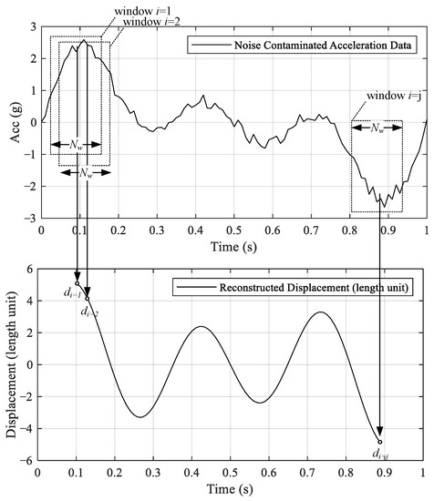
Figure 1. Illustration of displacement reconstruction scheme.

Lee et al. [22] adopted the central difference method to transfer the assumed displacement to acceleration, in which the reconstructed displacement does not contain noise. Instead of using the central difference method, the Newmark-beta method is utilized in this study to explore the possibility of enhancing the accuracy in displacement reconstruction. Equations (1) and (2) show the Newmark-beta equations, where $x_i$, ${\dot{x}}_i$, and ${\ddot{x}}_i$ are the displacement, velocity, and acceleration, respectively. $\Delta t$ refers to the time interval, $\gamma$ and $\beta$ are the Newmark constants. In this study, $\gamma$ and $\beta$ are taken as 1/2 and 1/6, respectively. Such assumption represents a linear acceleration process:

$${\dot{x}}_{i+1}={\dot{x}}_i+\Delta t\left[\left(1-\gamma \right){\ddot{x}}_i+\left(\gamma \right){\ddot{x}}_{i+1}\right]$$

(1)

$$x_{i+1}=x_i+\left(\Delta t\right){\dot{x}}_i+\Delta t^2\left[\left(0.5-\beta \right){\ddot{x}}_i+\left(\beta \right){\ddot{x}}_{i+1}\right]$$

(2)

Equation (1) could be rewritten in a matrix form, as indicated in Equation (3). As shown in Equation (3), matrix a is a set of acceleration data, and in the proposed algorithm, matrix a is the measured acceleration while L_d and L₂ are the constant. The dimension of the matrix a is adjusted to be the same length as each window (from i = 1 to N_w). Thus, the size of matrix L_d and matrix L₂ are N_w × (N_w + 1) and N_w × N_w, respectively. Matrix v in Equation (3) can be considered as the reconstructed velocity. However, it is understood that the exact solution for v is not possible.

$$L_{d}v-L_{2}a=0$$

(3)

where:

$$\begin{gathered} L_{\mathrm{d}}=\left[\begin{array}{ccccccc}-1& 1& & & & & \\ & -1& 1& & & 0& \\ & & & ........& & & \\ & 0& & & -1& 1& \\ & & & & & -1& 1\end{array}\right]L_2=\left[\begin{array}{ccccccc}(1-\gamma )\Delta t& \gamma \Delta t& & & & & \\ & (1-\gamma )\Delta t& \gamma \Delta t& & & 0& \\ & & & ........& & & \\ & 0& & & (1-\gamma )\Delta t& \gamma \Delta t& \\ & & & & & (1-\gamma )\Delta t& \gamma \Delta t\end{array}\right] \\ {v=\left[\begin{array}{ccccc}{\dot{x}}_i& {\dot{x}}_{i+1}& {\dot{x}}_{i+2}& .& .\end{array}\right]}^T a={\left[\begin{array}{ccccc}{\ddot{x}}_i& {\ddot{x}}_{i+1}& {\ddot{x}}_{i+2}& .& .\end{array}\right]}^T \end{gathered}$$

To find the reconstructed velocity, Equation (3) could be transformed into a minimization problem as described in Equation (4). Setting the first derivation with respect to v equals to zero, leading to a new equation, as indicated in Equation (5).

$$Min \left(v\right)={\Vert L_{d}v-L_{2}a\Vert }^2$$

(4)

$$v={L_d}^{-1}{L}_{2}a$$

(5)

Similarly, Equation (3) can be translated to a matrix form, as shown in Equation (6), in which the size of L₃ is N_w × N_w.

$$L_{d}u-\left(\Delta t\right)v-L_{3}a=0$$

(6)

where:

$$\begin{gathered} L_3=\left[\begin{array}{ccccccc}\left(0.5-\beta \right)\Delta t^2& \beta \Delta t^2& & & & & \\ & \left(0.5-\beta \right)\Delta t^2& \beta \Delta t^2& & & 0& \\ & & & ........& & & \\ & 0& & & \left(0.5-\beta \right)\Delta t^2& \beta \Delta t^2& \\ & & & & & \left(0.5-\beta \right)\Delta t^2& \beta \Delta t^2\end{array}\right] \\ u=\left[\begin{array}{ccccc}{x}_i& x_{i+1}& x_{i+2}& .& .\end{array}\right] \end{gathered}$$

where L₃ is a constant and u is defined as the reconstructed displacements, details of obtaining u are provided below. Again, Equation (6) can be considered as a minimization problem as well, in which the objective is formulated, as shown in Equation (7). Equation (7) is differentiated with respect to u to have Equation (2). Using v in Equation (5) and combining it with Equation (8), one can have Equation (9), which is the formula of reconstructed displacement with measured acceleration (a) data as input.

$$Min\left(u\right)={\Vert L_{d}u-\left(v\Delta t+L_{3}a\right)\Vert }^2$$

(7)

$$u=L_d{}^{-1}\left(v\Delta t+L_{3}a\right)$$

(8)

$$u=L_d{}^{-1}\left[\left(L_d{}^{-1}{L}_{2}a\right)\Delta t+L_{3}a\right]$$

(9)

The Thikonov regularization is often used to tackle the ill condition of the matrix inverse problem encountered from the reconstruction process. In this study, instead of using Thikonov regularization, Moore–Penrose pseudo inverse is utilized to handle the inverse of matrix L_d. Please note that although Equation (9) yields a set of displacements, only the middle point will be taken as the reconstructed displacement, then the window will continue to slide to obtain another reconstructed displacement. For a given window, the constructed displacement at the middle is the most accurate one among others. To ensure accuracy, a window-sliding technique is utilized wherein each window, only the outcome at the mid-point data is used. That is, for each window operation, a single point is obtained as the reconstructed displacement.

Besides acceleration data, another parameter needed for Equation (9) is the window size (N_w). N_w is affected by the frequency and interval time of acceleration records. To determine the size of N_w, this study utilizes a metaheuristic optimization technique to determine the appropriate N_w value for each frequency and interval. A single degree of freedom (SDOF) structure with various frequencies from 1–10 Hz with an increment of 1 Hz is generated, in which the accelerations are recorded in different time intervals such as 0.005 s, 0.01 s, and 0.02 s. As a result, 30 different cases are generated, and each SDOF structure is excited by the El Centro earthquake, as shown in Figure 2. Figure 3 shows the ground accelerations of El Centro. Since the structure and excited vibration are given, the exact displacement and acceleration of the structure can be calculated using the numerical integration method. The calculated structural accelerations are then added with noise and transformed to displacements using Equation (9). The added noise is an arbitrary random wave with frequencies between 1 to 200 Hz. In addition, the maximum amplitude of the added noise is twice the absolute mean of structural accelerations.

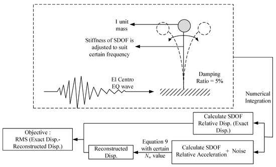
Figure 2. Determination of N_w using optimization and single degree of freedom (SDOF).

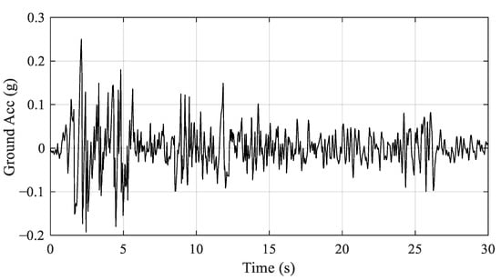
Figure 3. Ground acceleration of El Centro.

Metaheuristic optimization is performed to find the most suitable N_w value for each case. As illustrated in Figure 2, the objective of the optimization is to minimize root-mean-square error (RMSE) between exact and reconstructed displacements. Symbiotic organism search (SOS) [23] is used in this study. Although metaheuristic optimization probably needs more computational time compared to that of the conventional gradient-based optimization, metaheuristic optimization could avoid to trap at a local minimum point. Table 2 summarizes the metaheuristic optimization used in this study, including the values of parameters adopted. Figure 4 shows the optimization results of using the SOS algorithm. Based on the power regression lines, the formula for the N_w value could be formulated as shown in Equation (10), where f is the frequency of acceleration and Δt is interval time.

$$N_w=\frac{1}{\Delta t}{f}^{-8.9\Delta t-1}$$

(10)

Table 2. Summary of metaheuristic optimization used in this study.

Optimization Method	SOS Algorithm
Number of swarms	20
Number of iteration	50
Design variable	Window size (Nw)
Objective	Minimization of RMS between exact and reconstructed displacements

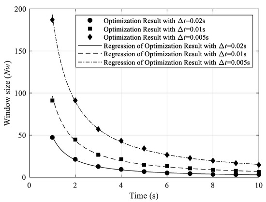
Figure 4. Optimization results of N_w value with respect to various frequencies and interval times.

Please note that the value of f in Equation (10) only has a moderate influence on the reconstructed displacement. Therefore, an approximate value of the fundamental frequency is often enough. To be specific, it should be acceptable to use a value of f with a 10% error. Using the generated 30 cases, the proposed problem is compared to the previous work by H.S. Lee et al. Table 3 shows the required N_w values for the proposed and the literature methods, respectively. It is seen that the proposed method requires less N_w that lessens the computational cost, and reduces the effect of time lag. In addition to the cost, Table 4 shows that the proposed method also delivers displacements with higher accuracy. It is seen that the performance of the current algorithm is able to reduce the required window size and enhance the accuracy of constructed displacement compared to literature. The current algorithm incorporates the Newmark-Beta as the main component to construct the displacement and utilizes the Moore–Penrose pseudo inverse to tackle the non-symmetrical inverse problem. While the window size is optimized using symbiotic optimization search (SOS). However, it is difficult to distinguish the contribution of each component to the increase in performance.

Table 3. Comparison of window size (N_w) between the proposed and the literature methods [22].

	Window Size (Nw)
Frequency	Literature [22]			Proposed Formula
	Δt = 0.02 s	Δt = 0.01 s	Δt = 0.005 s	Δt = 0.02 s	Δt = 0.01 s	Δt = 0.005 s
1	150	300	600	50	100	200
2	75	150	300	22	47	97
3	50	100	200	14	30	63
4	38	75	150	10	22	47
5	30	60	120	8	17	37
6	25	50	100	6	14	31
7	21	43	86	5	12	26
8	19	38	75	4	10	23
9	17	33	67	4	9	20
10	15	30	60	3	8	18

Table 4. Root-mean-square error (RMSE) between the proposed and the literature methods [22].

Freq.	Error in the Literature (1 × 10−3)			Error in the Proposed (1 × 10−3)
	Δt = 0.02 s	Δt = 0.01 s	Δt = 0.005 s	Δt = 0.02 s	Δt = 0.01 s	Δt = 0.005 s
1	7.27	6.67	6.5	5.41	4.36	4.18
2	3.74	3.09	3.05	1.52	1.41	1.41
3	1.95	1.65	1.6	0.73	0.65	0.63
4	1.29	1	0.89	0.5	0.41	0.38
5	0.89	0.69	0.57	0.38	0.25	0.24
6	0.65	0.44	0.39	0.27	0.19	0.18
7	0.46	0.35	0.28	0.19	0.15	0.14
8	0.37	0.28	0.21	0.17	0.11	0.11
9	0.31	0.2	0.17	0.19	0.09	0.08
10	0.24	0.17	0.13	0.13	0.08	0.07

2.2. MEMS Accelerometer and NB-IoT Technology

As described earlier, to have continuous or stable records in the period of the bridge health monitoring, NB-IoT technology is utilized to transmit the acceleration signals from the bridge site to the server. In this study, the ADXL355 acceleration sensor is used, as shown in Figure 5a. ADXL is selected due to its affordable cost and its adequate ability to sense the motion of the bridge. ADXL355 requires power around 3.6 V and has a sensing range of ±3 g that is suitable for this study. The sampling frequency is 125 Hz, and the working temperature is from −40 °C up to 125 °C, which is suitable for bridge monitoring tasks. The acceleration sensor ADXL355 is mounted to Nordic Semiconductor nRF9160, as shown in Figure 5b that will read the input signal from the sensor.

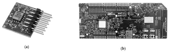
Figure 5. (a) ADXL 335 accelerometer; (b) Nordic Semiconductor nRF9160.

nRF9160 is equipped with long term evolution (LTE) with bandwidth 700–960 MHz and 1710–2200 MHz that will send the signal to base transceiver station (BTS) and to the off-site server as shown in Figure 6. The low-cost sensor and NB-IoT package with low power requirements enable the bridge monitoring to be performed at an acceptable price at length.

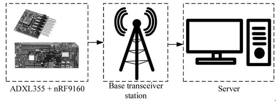
Figure 6. General scheme of signal transmission from an on-site sensor to an off-site server.

2.3. Proposed Level 1 and Level 2 Damage Detection

This section explains the proposed method that intends to detect damage occurrence and location. The proposed method utilizes the displacement reconstruction algorithm explained in an earlier section. In the bridge monitoring task, accelerometers often spread along a bridge span, as illustrated in Figure 7. Assuming that i number of sensor points (SP) spread along a bridge, as shown in Figure 7 and each sensor records acceleration data. If there is damage occurred, the collected accelerations naturally include two sets of records. Namely, the original and observed sets. These two sets of accelerations are then transformed into reconstructed displacements (RDisp) using Equation (10). The root-mean-square (RMS) of RDisp for each sensor point (RMSD_i) is calculated as formulated in Equation (11).

$$RMS{D}_i=\sqrt{\frac{{\displaystyle \sum _{j=1}^{all}RDis{p}^2\left(j\right)}}{n}}$$

(11)

where n is the quantity of data.

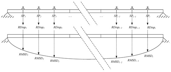
Figure 7. Illustration of sensor points and damage index 1.

Each original and observed sets consist of i number of RMSD, and for either set and is normalized with its own maximum value if shown by a diagram with respect to the sensor position will create a deflection shape as shown in Figure 7. Level 1 damage indicator is the shape difference between the original and observed RMSDs, as shown in Figure 8. Once there is a significant difference between these two RMSDs, the bridge will be diagnosed as a damaged one. The larger the damage indicator, the more severely damaged the bridge. A threshold could be suggested based on available data. As shown in Figure 8, the difference between two RMSDs at the SP₄ position is zero since two sets of data are normalized with respect to the same midpoint.

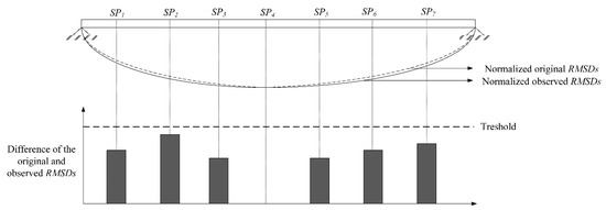
Figure 8. Illustration of Level 1 damage indicator.

For Level 2 damage indicator, the dRMSD, which is the difference between adjacent RMSDs as formulated in Equation (12), is calculated ( $RMS{D}_i \mathrm{is} \mathrm{Zero}$ ). Same as Level 1 damage indicator, original and observed dRMSDs are computed as illustrated in Figure 9. Subsequently, the difference between original and observed dRMSDs are plotted with respect to the sensor point, as shown in Figure 9. Each segment of the bridge is represented by a single value of damage indicator (i.e., dRMSD) and If one of the values is particularly prominent, indicating that a particular segment is in a damaged status. The more sensors, the more accurate in locating the damaged position.

$$dRMSD=\left[\begin{array}{l}\left|RMS{D}_1\right|,\left|RMS{D}_2-RMS{D}_1\right|,\left|RMS{D}_3-RMS{D}_2\right|,\dots ,\\ \left|RMS{D}_i-RMS{D}_{i-1}\right|\end{array}\right]$$

(12)

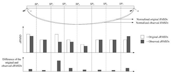
Figure 9. Illustration of Level 2 damage indicator.

3. Bridge Health Monitoring Experiment

To validate the aforementioned displacement reconstruction method and damage indicators, three different experiments are introduced in this section.

3.1. Small-Scale Bridge with Vibration Induced by Passing Vehicle

3.1.1. Experiment Setup

The experiment setup is shown in Figure 10, where the bridge has a 5.6 m span. During the testing, the excitation of the bridge is induced by a moving cart on the bridge span, as indicated in Figure 10. MEMS accelerometer with a sampling rate of 125 Hz and LVDT with a sampling rate of 200 Hz is equipped at the first quarter, middle, and the third quarter of the bridge as shown in Figure 10.

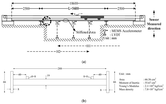
Figure 10. (a) General scheme of a small-scale bridge with passing vehicles; (b) cross-section of section A-A.

For bridge frequency, the span length of small scale bridge is set so that its first three mode frequencies are 3.7 Hz, 15 Hz, and 30 Hz, respectively. As shown, these three frequencies are reasonable compared to those of a real bridge. For the mass ratio, two different types of ratios are used: light and heavy. The bridge weight is 291 kg, and the weights of vehicles are 30 kg and 47 kg, respectively. The mass ratio for the light case is around 10%, and the mass ratio for the heavy case is 16%. The heavy case is intended to model two consecutive trucks or a trailer truck with full loading. For the length ratio, the light case is 7%, and the heavy case is 16%. For the speed ratio (α), the similarity ratio adopted is described in Equation (13), where v is the vehicle speed (m/s), f refers to the fundamental frequency (Hz), and l_b is bridge span length (m). Assuming the real bridge has 40 m in span and 3.7 Hz of the fundamental frequency, in this case, the small scale vehicle speeds of 0.4, 0.8, and 1.2 m/s are equivalent to 10, 20, and 30 km/h for a real bridge

$$\alpha =\frac{v}{\left(2.f.l_b\right)}$$

(13)

To simulate various conditions of bridge and passing vehicle, 12 different scenarios are designed as indicated in Table 5. Two different bridge conditions are used, namely the original and the stiffened ones. The stiffened bridge refers to a stiffener is attached to one of the bridge spans to increase its stiffness, as shown in Figure 11b. Figure 10a indicates the location of the stiffened span. Two vehicles with different weights are used, namely heavy and light carts. The weights are 30.4 kgf and 47.3 kgf for the light and heavy carts, respectively. Three different speeds are used, and they are 0.4, 0.8, and 1.2 m/s, respectively. In total, 12 different scenarios are considered as listed in Table 5. For each scenario, the test will be repeated 10 times; each time, the cart will run back and forth once, as shown in Figure 10a.

Table 5. List for small scale bridge experiments.

No	Scenario Name	Bridge Type	Vehicle Mass	Vehicle Speed (m/s)
1	LVB0S1	Original	Light	0.4
2	LVB0S2	Original	Light	0.8
3	LVB0S3	Original	Light	1.2
4	HVB0S1	Original	Heavy	0.4
5	HVB0S2	Original	Heavy	0.8
6	HVB0S3	Original	Heavy	1.2
7	LVB1S1	Stiffened	Light	0.4
8	LVB1S2	Stiffened	Light	0.8
9	LVB1S3	Stiffened	Light	1.2
10	HVB1S1	Stiffened	Heavy	0.4
11	HVB1S2	Stiffened	Heavy	0.8
12	HVB1S3	Stiffened	Heavy	1.2

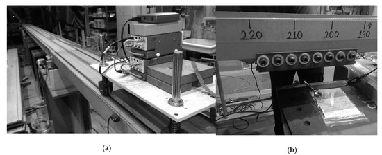
Figure 11. (a) Small scale bridge experiment; (b) a bridge span with a stiffened plate.

Table 6 shows the dynamic bridge properties, such as the first three frequencies for the original and stiffened bridges. It is seen that although this is a small scale bridge, its dynamic property is adjusted so that it is similar to an actual bridge condition. In Table 6, frequency is measured under free vibration 5 times. It is shown that the stiffened bridge only slightly increases its frequency from 3.733 to 3.867 Hz. Table 6 also displays the coefficient of variation (cov) among 5 testing data. It is shown that covs are very small, indicating the measurement is very accurate. Table 7 shows the damping ratio for the original and stiffened bridges under free vibration. Similar to frequency measurement, the number of measurements is 5.

Table 6. Bridge frequency for the first three modes.

	Original Bridge				Stiffened Bridge
Mode	Frequency Statistical Properties (Hz)				Frequency Statistical Properties (Hz)
	Max.	Min.	Mean	cov	Max.	Min.	Mean	cov
1	3.733	3.733	3.733	0	3.867	3.867	3.867	0
2	15.067	14.933	14.987	0.005	14.533	14.533	14.533	0
3	32.000	29.600	30.800	0.037	31.867	30.667	31.493	0.015

Table 7. Damping ratio for original and stiffened bridges.

Bridge	First Mode Damping Ratio Statistical Properties
	Max.	Min.	Mean	cov
Original	0.025	0.019	0.023	0.114
Stiffened	0.018	0.016	0.017	0.047

3.1.2. Level 1 Detection Using Frequency

From 10 experiments of each scenario, statistics of the fundamental frequency are shown in Table 8. The fundamental frequency is calculated using the direct fast Fourier transform (FFT). Mean, Maximum, and Minimum among 10 experiments are presented. It is shown that frequencies are changed accordingly due to varied vehicle speeds and masses. The increasing vehicle can reduce the fundamental frequency while increasing vehicle mass tends to decrease fundamental frequency. In addition, the position of the vehicle also could affect the mass matrix of the entire bridge, resulting in a different frequency. For the current state, this study only reports the phenomena found in our small scale experiment; no further statement is concluded for other small scale or real bridge conditions.

Table 8. Fundamental frequency for each case.

Scenario	Frequency Mode 1 Statistical Properties (Hz)
	Max.	Min.	Mean	cov
LVB0S1	4.027	3.973	4.002	0.004
LVB0S2	3.978	3.822	3.9	0.021
LVB0S3	3.927	3.293	3.58	0.073
HVB0S1	4.069	3.997	4.02	0.008
HVB0S2	3.964	3.809	3.871	0.021
HVB0S3	3.894	3.622	3.821	0.031
LVB1S1	4.057	4.003	4.035	0.005
LVB1S2	3.994	3.864	3.97	0.01
LVB1S3	3.931	3.84	3.883	0.01
HVB1S1	4.086	3.908	3.979	0.011
HVB1S2	3.956	3.801	3.816	0.013
HVB1S3	3.925	3.623	3.847	0.029

Instead of using direct FFT, FFT with window is performed. Results of windowed FFT are normalized to 1. Figure 12 and Figure 13 show the displacements and FFT spectrogram for scenario LVB0S1 and LVB0S3, respectively. Figure 12 and Figure 13 contain three plots. The first plot shows the dynamic displacement at mid-span under a moving load where the static displacement has been filtered out, and the second plot shows the FFT spectrogram, where each window contains 1000 data and 999 of them are overlapped with the next windows. The third plot presents two FFTs at different times indicated in the second plot. Figure 12 and Figure 13 show that different cart positions could yield different fundamental frequencies. Using frequency as a bridge health indicator with passing vehicles should be cautious.

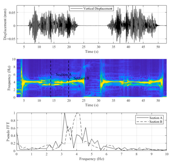
Figure 12. Windowed fast Fourier transform (FFT) of LVB0S1.

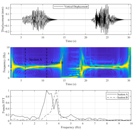
Figure 13. Windowed FFT of LVB0S3.

3.1.3. Level 1 Detection Using Reconstructed Displacements

This subsection introduces the results of the Level 1 detection using reconstructed displacements explained in Section 2.1. As described, both MEMS accelerometers and LVDT are used for measurement, as shown in Figure 10a; comparisons between two devices are conducted to validate the accuracy of the proposed approach. Figure 14 and Figure 15 (top) shows the measured accelerations using MEMS for scenarios of LVB0S1 and LVB0S3, respectively. Figure 14 and Figure 15 (bottom) shows the displacements from LVDT and reconstructed displacement using MEMS for scenarios of LVB0S1 and LVB0S3, respectively. It is shown that reconstructed displacement is almost identical to those of LVDT. Note that noise has been filtered out in the reconstructed displacements.

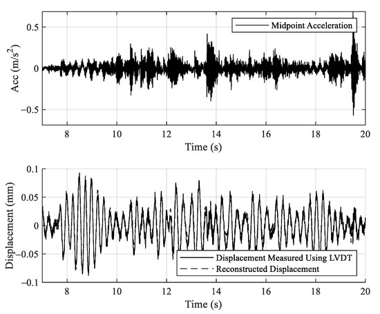
Figure 14. Linear variable differential transformers (LVDT) displacements and reconstructed displacements (bottom) from accelerations (top) on scenario LVB0S1.

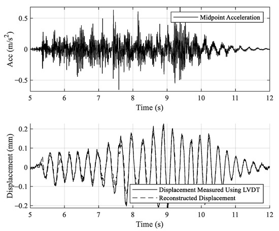
Figure 15. LVDT displacements and reconstructed displacements (bottom) from accelerations (top) on scenario LVB0S3.

As shown in Figure 10, three accelerometers are attached to the bridge. To demonstrate the proposed approach, the mean value of RMSDs between original and stiffened bridges in the H1 direction is compared with those of the H2 direction. Figure 16 shows the mean RMSDs in H1 and H2 directions for (a) original (Cases 1 to 6) and (b) stiffened bridge (Cases 7 to 12). Points No. 1 and No. 5 represent the two ends of the test bridge, while points No. 2, No. 3, and No. 4 represent the sensor location at the first, second, and third quarters of the bridge. Figure 16 (top) clearly shows that the shapes created by the RMSD value have no significant change between H1 and H2 directions since both plots have identical conditions (only the cart moving direction is opposite). Level 1 damage indicator between H1 and H2 directions is less than 5 × 10⁻³. However, if the Level 1 damage indicator is compared between the original and stiffened bridges, the shapes are quite different from those of Figure 16. As shown in Figure 17, the Level 1 damage indicator is around 1.8 × 10⁻² up to 3.5 × 10⁻². The proposed indicator could recognize the occurrence of the stiffened plate while the frequency indicator could not. Need to be noted, the comparison is performed between Cases 1 to 6 and Cases 7 to 12 to reproduce the actual bridge conditions, in which a bridge is often passed by various vehicle types and vehicle speeds.

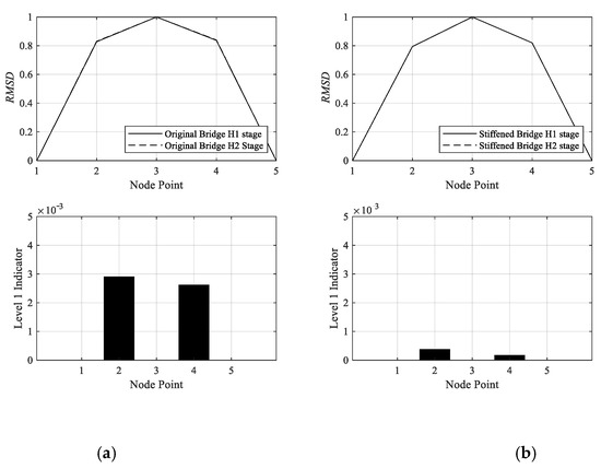
Figure 16. Level 1 damage indicator of (a) original bridge with H1 and H2 directions; (b) stiffened bridge with H1 and H2 directions.

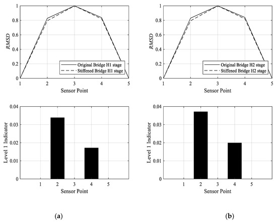
Figure 17. Level 1 damage indicator of (a) original and stiffened bridges in H1 direction; (b) original and stiffened bridges in H2 direction.

3.2. Analysis of a Numerical Bridge

In this section, a numerical model is created to demonstrate the proposed method in recognizing the damage position for a given bridge, that is, the Level 2 damage detection. Because the accuracy of Level 2 damage detection depends on the number of sensors, a numerical model is more convenient to fulfill this requirement and is therefore adopted here. Only the vertical direction is considered in the numerical model. Both ends are fixed. Mass and stiffness are divided into 200 increments, and 9 sensors are uniformly distributed along the span. Figure 18 shows the bridge dimension and accelerometer positions. As shown, on a 40-m bridge, sensors are arranged every 4 m. The bridge consists of 200 finite elements with assigned mass and stiffness. For the given mass and stiffness, the mass and stiffness matrix could be constructed, and together with the damping matrix, the governing equation is displayed in Equation (13). The bridge property is listed in Table 9.

$$M\ddot{x}\left(t\right)+C\dot{x}\left(t\right)+Kx\left(t\right)=M{\ddot{x}}_a$$

(14)

where M, C, and K are the structural mass, damping, and stiffness matrix, respectively. Dynamic analysis is conducted using the state–space method provided by MATLAB SIMULINK, where only displacement in the gravity direction is calculated. The vibration source in this numerical analysis is ambient vibration (${\ddot{x}}_a$), which is simulated by white noise with a frequency ranging from 1 to 10 Hz. Figure 19 shows the first three modes of the bridge, where the frequencies of the first three modes are 3.497, 6.994, and 10.490 Hz, respectively.

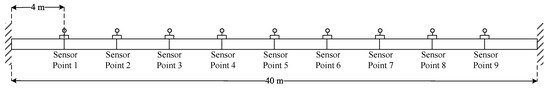
Figure 18. Configuration of numerical bridge model.

Table 9. Bridge properties.

Bridge Property	Value	Unit
Young’s modulus	20,000	MPa
Moment inertia	3.27 × 105	mm4
Total weight	10	tonf

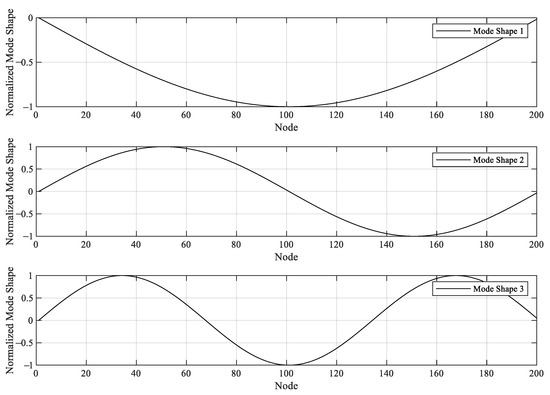
Figure 19. The first three mode shapes of a numerical bridge.

To demonstrate the proposed Level 2 damage detection method, 6 cases of damage scenario are artificially created as listed in Table 10. In cases 1 to 4, a bridge with single damage is considered. On the other hand, a bridge with two damages is considered in cases 5 and 6. The damage is generated by reducing the stiffness of the original bridge by a factor of 0.9 with one-meter-long, as shown in Table 10. For each damage case, the obtained acceleration data from original and damage bridges are used to calculate the Level 2 damage indicator. Figure 20, Figure 21, Figure 22, Figure 23, Figure 24 and Figure 25 display the Level 2 damage indicators for each case, indicating that the proposed Level 2 indicator is able to provide a promising prediction for the damage location, either with a single or double damages.

Table 10. Damage case for a numerical bridge.

Case	Damage Location
1
2
3
4
5
6

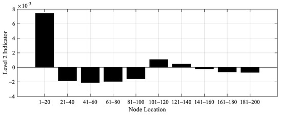
Figure 20. Level 2 damage indicator for Case 1.

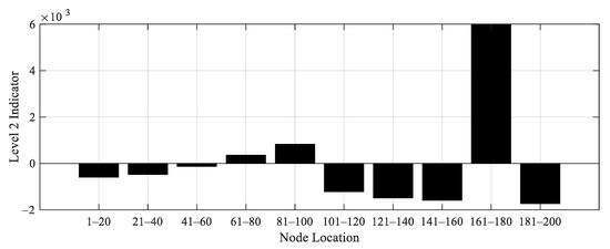
Figure 21. Level 2 damage indicator for Case 2.

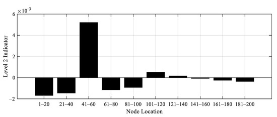
Figure 22. Level 2 damage indicator for Case 3.

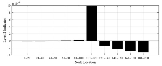
Figure 23. Level 2 damage indicator for Case 4.

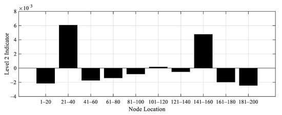
Figure 24. Level 2 damage indicator for Case 5.

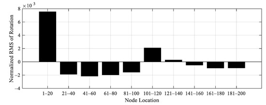
Figure 25. Level 2 damage indicator for Case 6.

3.3. Full-Scale Bridge Experiment

A full-scale bridge is used to demonstrate the implementation of the proposed Level 1 damage detecting method. Wenzhou Bridge, located in Taipei city, is selected as the test bridge because it is an important bridge, and the riverside park under the bridge provides test personnel to facilitate the assembly of test equipment. Wenzhou bridge is constructed in the Year 2000. It is a prestressed girder bridge with four lanes. No damage is visually detected before our testing. The experiments are initiated at the beginning of April 2020, and field data are continuously collected until now. Due to lack of information and based on the visual inspection, the status of the bridge in April 2020 is assumed to be in a healthy condition. Wenzhou Bridge is an RC prestress girder bridge with dimensions shown in Figure 26. Accelerometers integrated with NB-IoT are attached along the bridge span at the first, second, and third quarters. The power of the equipment is supported by several detached batteries that need to be refilled regularly. The sampling rate is 125 Hz, and acceleration data are recorded every 12 min. Each record consists of 4096 points. That is, each record is approximately 33 s-long. The collected acceleration data are transformed into displacements based on the proposed algorithm. Because the proposed reconstructed displacement algorithm requires the bridge’s fundamental frequency, FFT analysis is first performed to obtain the frequency, as shown in Figure 27. It is seen that a technical problem occurred from 6/15 to 6/30 (month/date), causing a gap in collecting data. However, such a gap does not affect the following analysis. The frequency of the bridge is assumed to be 4 Hz that is calculated based on the mean of the calculated FFTs. As explained in Section 3.1.2, different frequencies are observed, as shown in Figure 27, where the frequency is ranging from 3.5 Hz to 4.5 Hz.

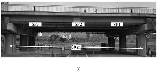
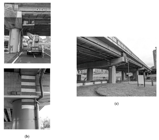
Figure 26. (a) Sensor positions and bridge dimension; (b) power supply for accelerometer and NB-IoT; (c) side view of Wenzhou bridge.

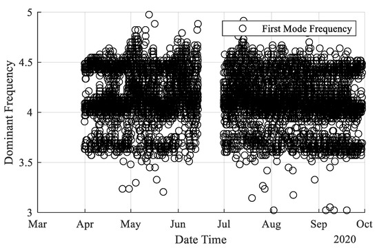
Figure 27. Calculated fundamental frequencies for each set of data.

When applying the proposed Level 1 damage detection to the Wenzhou Bridge, the condition in April is assumed to be the original condition, which is considered as a reference point for calculating the Level 1 damage indicator. Damage indicator is calculated for each month except June. Figure 28, Figure 29 and Figure 30 show the Level 1 damage indicator for the Wenzhou Bridge. It is shown that the bridge still remains in the same condition as that in April. Figure 28, Figure 29, Figure 30 and Figure 31 depict the proposed Level 1 indicator by comparing the normalized RMSD in April. If the difference is large, indicating that there is damage occurrence. As shown, the largest RMSD difference is 8 × 10^−3, which is considered a relatively small value compared to those of the small-scale experiments. It is, therefore, concluded that the bridge condition from May to September does not significantly change from April.

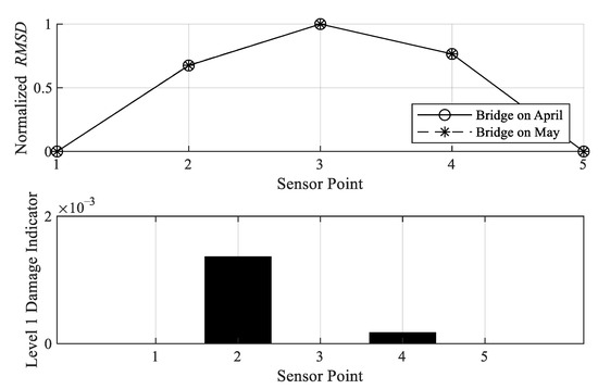
Figure 28. Level 1 damage indicator of Wenzhou bridge in May.

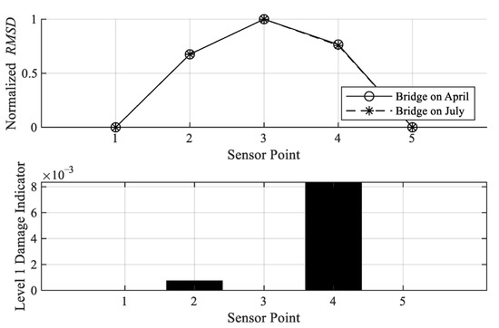
Figure 29. Level 1 damage Indicator of Wenzhou Bridge in July.

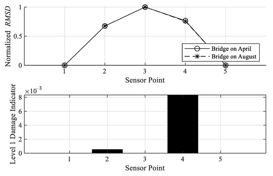
Figure 30. Level 1 damage indicator of Wenzhou bridge in August.

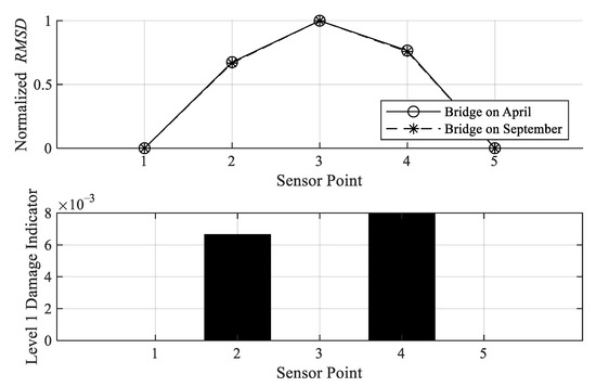
Figure 31. Level 1 damage indicator of Wenzhou bridge in September.

4. Conclusions

This study introduces a novel approach for bridge health monitoring utilizing a displacement reconstruction algorithm. The algorithm is developed utilizing the Newmark-beta method, the Moore–Penrose pseudo inverse and the sliding window technique. Level 1 and Level 2 damage detections are considered in this study. Three experiments are carried out to validate and demonstrate the proposed method. Several brief conclusions and discussions could be drawn as described below:

• The proposed displacement reconstruction algorithm requires less computational time and has higher accuracy compared to the previous study, as provided in Section 2.1. The input parameters of the proposed algorithm are recorded accelerations, fundamental frequency and window size;
• Level 1 damage detection is performed by first using FFT to identify the fundamental frequency of a bridge. It is shown that various vehicle weights and velocities could affect the dominant frequency. Window-slide FFT is also performed to examine the variation of the dominant frequency per window, and it shows that dominant frequency varies as different vehicle position and speed;
• Although the stiffness difference between the original and the stiffened bridge in the small-scale bridge experiment is slight, the proposed Level 1 damage detection using reconstructed displacement is able to distinguish the difference between the two;
• The proposed Level 2 damage detection is successfully to predict the damage location for either case: single or double damages for the numerical examples;
• To apply the proposed damage detection approach to an actual bridge, MEMS accelerometer and NB-IoT are integrated with the proposed methodology. On-site monitoring was conducted from April until November. Based on the proposed Level 1 damage detection, the monitored bridge shows no indication of degradation since April. The proposed method enables on-site monitoring to be conducted without interrupting traffic activity at an acceptable cost.

Please note that the input of the proposed reconstructed displacement algorithm is the measured accelerations. That is, the proposed method cannot consider the effect of each individual factor, including environmental factors, separately. However, the effects of the environmental factors are included in the measured data, and the corresponding influences are considered. In addition, in a real case, the deformation of a bridge is in 3 directions. Although most failure modes are related to the vertical deflection, some failure modes, such as shear failure, is not, and the proposed method may not be suitable in such case. The proposed method is only suitable for a bridge with failure mode related to the gravity direction. The current approach could only provide an early warning for a bridge system. A mechanical-based model is needed to further clarify the possible failure mechanisms for a bridge.

References

- Rytter, A. Vibrational Based Inspection of Civil Engineering Structures. Ph.D. Thesis, Department of Building Technology and Structural Engineering, Aalborg University, Aalborg, Denmark, 1993. [Google Scholar]
- Schommer, S.; Nguyen, V.H.; Maas, S.; Zürbes, A. Model updating for structural health monitoring using static and dynamic measurements. Procedia Eng. 2017, 199, 2146–2153. [Google Scholar] [CrossRef]
- Yu, S.; Ou, J. Structural Health Monitoring and Model Updating of Aizhai Suspension Bridge. J. Aerosp. Eng. 2017, 30. [Google Scholar] [CrossRef]
- Lee, Y.-J.; Cho, S. SHM-Based Probabilistic Fatigue Life Prediction for Bridges Based on FE Model Updating. Sensors 2016, 16, 317. [Google Scholar] [CrossRef]
- Zong, Z.; Lin, X.; Niu, J. Finite element model validation of bridge based on structural health monitoring—Part I: Response surface-based finite element model updating. J. Traffic Transp. Eng. 2015, 2, 258–278. [Google Scholar] [CrossRef]
- Farrar, C.R.; Jauregui, A.D. Comparative study of damage identification algorithms applied to a bridge: I. Experiment. Smart Mater. Struct. 1998, 7, 704–719. [Google Scholar] [CrossRef]
- Mehrjoo, M.; Khaji, N.; Moharrami, H.; Bahreininejad, A. Damage detection of truss bridge joints using Artificial Neural Networks. Expert Syst. Appl. 2008, 35, 1122–1131. [Google Scholar] [CrossRef]
- Neves, A.C.; González, I.; Leander, J.; Karoumi, R. Structural health monitoring of bridges: A model-free ANN-based approach to damage detection. J. Civ. Struct. Health Monit. 2017, 7, 689–702. [Google Scholar] [CrossRef]
- Li, Z.H.; Au, F.T.K. Damage Detection of a Continuous Bridge from Response of a Moving Vehicle. Shock Vib. 2014, 2014, 1–7. [Google Scholar] [CrossRef]
- Li, H.-N.; Li, D.-S.; Song, G.-B. Recent applications of fiber optic sensors to health monitoring in civil engineering. Eng. Struct. 2004, 26, 1647–1657. [Google Scholar] [CrossRef]
- Wong, K.-Y. Instrumentation and health monitoring of cable-supported bridges. Struct. Control Health Monit. 2004, 11, 91–124. [Google Scholar] [CrossRef]
- Huseynov, F.; Kim, C.; Obrien, E.; Brownjohn, J.; Hester, D.; Chang, K. Bridge damage detection using rotation measurements—Experimental validation. Mech. Syst. Signal Process. 2020, 135, 106380. [Google Scholar] [CrossRef]
- Zhang, Q.W. Statistical damage identification for bridges using ambient vibration data. Comput. Struct. 2007, 85, 476–485. [Google Scholar] [CrossRef]
- Liao, A.S.; Kiremidjian, R.; Loh, C.-H. Structural damage detection and localization with unknown post-damage feature distribution using sequential change-point detection method. J. Aerosp. Eng. 2019, 32, 04018149. [Google Scholar] [CrossRef]
- Zhang, S.; Liu, Y. Damage Detection in Beam Bridges Using Quasi-Static Displacement Influence Lines. Appl. Sci. 2019, 9, 1805. [Google Scholar] [CrossRef]
- Zeinali, Y.; Story, B.A. Impairment localization and quantification using noisy static deformation influence lines and Iterative Multi-parameter Tikhonov Regularization. Mech. Syst. Signal Process. 2018, 109, 399–419. [Google Scholar] [CrossRef]
- Zeinali, Y.; Story, B.A. Framework for Flexural Rigidity Estimation in Euler-Bernoulli Beams Using Deformation Influence Lines. Infrastructures 2017, 2, 23. [Google Scholar] [CrossRef]
- Mei, Q.; Gül, M.; Boay, M. Indirect health monitoring of bridges using Mel-frequency cepstral coefficients and principal component analysis. Mech. Syst. Signal Process. 2019, 119, 523–546. [Google Scholar] [CrossRef]
- Tennyson, R.C.; Mufti, A.A.; Rizkalla, S.H.; Tadros, G.; Benmokrane, B. Structural health monitoring of innovative bridges in Canada with fiber optic sensors. Smart Mater. Struct. 2001, 10, 560–573. [Google Scholar] [CrossRef]
- Yi, T.; Li, H.; Gu, M. Recent research and applications of GPS based technology for bridge health monitoring. Sci. China Ser. E Technol. Sci. 2010, 53, 2597–2610. [Google Scholar] [CrossRef]
- Cantero, D.; McGetrick, P.; Kim, C.; Obrien, E. Experimental monitoring of bridge frequency evolution during the passage of vehicles with different suspension properties. Eng. Struct. 2019, 187, 209–219. [Google Scholar] [CrossRef]
- Lee, H.S.; Hong, Y.H.; Park, H.W. Design of an FIR filter for the displacement reconstruction using measured acceleration in low-frequency dominant structures. Int. J. Numer. Methods Eng. 2010, 82, 403–434. [Google Scholar] [CrossRef]
- Cheng, M.-Y.; Prayogo, D. Symbiotic Organisms Search: A new metaheuristic optimization algorithm. Comput. Struct. 2014, 139, 98–112. [Google Scholar] [CrossRef]
Publisher’s Note: MDPI stays neutral with regard to jurisdictional claims in published maps and institutional affiliations. |
© 2020 by the authors. Licensee MDPI, Basel, Switzerland. This article is an open access article distributed under the terms and conditions of the Creative Commons Attribution (CC BY) license (http://creativecommons.org/licenses/by/4.0/).