Abstract
Study on viscoelastic properties of the multi-layered coarse-grained soil (CGS) is very important for safety assessment and disaster prevention of subgrade engineering. Current research work is mainly focused on the one-layered CGS and the actual pebble inclusion of irregular polyhedron is usually simplified as an ideal shape of sphere or ellipsoid. Very few studies are available for predicting viscoelastic parameters of the multi-layered CGS. In this paper, a new method is proposed to predict viscoelastic parameters of multi-layered CGS based on the homogenization method and elastic–viscoelastic corresponding principle, in which the interface-layer viscoelasticity and the actual shape of pebble inclusion are firstly taken into account. Research results show the creep deformation is decreased with the increase of the shape factor (ρ) of pebble inclusion, and the interface-layer height (h) and numbers (N). ρ is in the range of 1–1.8 and the suitable interface-layer height is 20–30% as much as the height of one-layered CGS. The tested creep curves of the multi-layered CGS agree well with the predicted ones and can prove the existence of the interface-layer (considering at least one interface-layer) and verify the validity of this new interface-layer method.
1. Introduction
Coarse-grained soil (CGS) consists of a pebble (with high elastic modulus) and sand–clay matrix (with rheological properties) surrounding the pebble and pore [1,2,3]. It is easily available in nature and thus widely applied in the subgrade, bridge foundation, and structure foundation engineering [4]. For improving the bearing capacity of the foundation, the CGS of different gradations needs to be artificially filled [5,6,7,8]. The slipping and embedding of different gradations CGS particles would lead to a certain height of interface-layer, i.e., the formation of multi-layered CGS [9,10,11]. Under long-term loading, the multi-layered CGS may cause uneven settlement due to its rheology properties (depending on its microscopic components and structure) and there exists a potential safety hazard for the foundation engineering [12]. Therefore, it is very important to determine the macroscopic rheological parameters of multi-layered CGS with consideration of the interface-layer for predicting its long-term deformation.
Currently, the macroscopic rheological parameters of materials are mainly studied by two theoretical methods: periodic cell method and homogenization method. Since the periodic cell method needs a representative volume unit of a periodic array, it is only used for most metallic alloy materials [13], ceramic material [14], and a few nonmetallic materials with periodic microstructures (e.g., concrete [15]). The homogenization method is widely applied for the geotechnical materials of a few periodic microstructures, with different solution methods. For example, Du et al. [16] and Chang et al. [17] calculated equivalent elastic moduli of the concrete and the sandy soil by hollow sphere model and three-phase sphere method, respectively. Wang [18] and Wang et al. [19] predicted equivalent viscoelastic parameters of the asphalt and the saturated frozen soils by Mori-Tanaka equivalent method and improved Hashin model combined with the elastic–viscoelastic corresponding principle. For the one-layered CGS, some solution methods, Hashin model method (Vallejo and Lobo [20]), Mori-Tanaka equivalent method (by Yang et al. [21]), two-phase model method (by Hu [22]), and numerical simulation method based on homogenization method (by Barbero et al. [23], Xu et al. [24], Li et al. [25]) were adopted to predict its elastic parameters. Its viscoelastic parameters could be also obtained by the elastic–viscoelastic corresponding principle. It is worth to note that in all of these homogenization methods, the inclusion (large pebble particles) were simplified to be an ideal sphere or ellipsoid particles, which is obviously inconsistent with the actual irregular shape of the inclusion (polyhedron). Besides, for the multi-layered materials, most works of literature were focused on laminate composites for predicting the elastic parameters [26,27] and rheological parameters [28] by the homogenization method, regardless of the interface-layers. Very few studies are available on theoretically studying the viscoelastic parameters of the multi-layered CGS.
In addition, triaxial compression test was also used to determine macroscopic elastic parameters of the one-layered CGS. Effects of different factors, content [29,30,31], and sizes [32,33] of the coarse pebble, content of the fine particles [34] on its elastic parameters were measured and analyzed by the statistic method and the estimation method, respectively. Hou et al. [35] adopted the triaxial creep test to measure the viscoelastic parameters of the one-layered CGS varying with the clay content. However, the multi-layered CGS is less studied experimentally.
This paper aims to propose a new method for predicting the viscoelastic parameters of multi-layered CGS with consideration of interface-layer and actual pebble inclusion shape. Firstly, the calculation model of one-layered CGS and multi-layered CGS with interface-layers were established by the homogenization method. Then, the effective elastic parameters of one-layered CGS, interface-layer and multi-layered CGS were calculated to obtain the viscoelastic parameters by elastic–viscoelastic corresponding principle. Finally, the predicted creep strains of the one-layered, two-layered, and three-layered CGS were verified by the triaxial creep tests.
2. Viscoelastic Parameter Model of the Multi-Layered CGS
2.1. Structure Model of the Multi-Layered CGS
Figure 1 shows a diagrammatic sketch of three-layered CGS composite structures with solid phase (pebble, sand–clay matrix) and gas phase (pore) of different gradations, where H is one-layered CGS height, and h1 and h2 are interface-layer height. For determining its macroscopic viscoelastic parameters, its macroscopic elastic parameters need to be firstly obtained based on homogenization principle. This includes four steps: (1) consider the solid phase (sand and clay as matrix, pebble as inclusion) for homogenizing the one-layer CGS without consideration of gas phase (pore), in order to obtain the effective elastic parameters (bulk and shear modulus) of the solid phase, (2) consider both the solid phase (as matrix) and the gas phase (pore as inclusion) for homogenization in order to obtain the elastic parameters (bulk and shear modulus) of the one-layered CGS, (3) consider the interface-layer as two one-layers with different gradations of the solid phase and the gas phase for homogenization, in order to obtain the elastic parameters (bulk and shear modulus) of the interface-layer, (4) superimpose the results of steps (2) and (3) to obtain the effective elastic modulus of multi-layered CGS. Then, apply the elastic–viscoelastic corresponding principle to obtain the viscoelastic parameters of multi-layered CGS, details as follows.
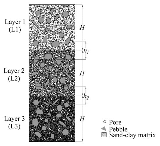
Figure 1.
Diagrammatic sketch model of multi-layered coarse-grained soil (CGS) structure.
2.2. Viscoelastic Parameter Model of One-Layered CGS
Effective elastic parameters of the one-layered CGS can be calculated by those of the solid phase with consideration of the gas phase (pore).
Figure 2 shows the calculation model of the solid phase for one-layered CGS, where Ωp is the region of pebble, Ωm is the region of sand–clay matrix and Ωeq is the region of equivalent media. The pebble is first simplified as isotropic sphere inclusion and completely surrounded by the isotropic sand–clay matrix.
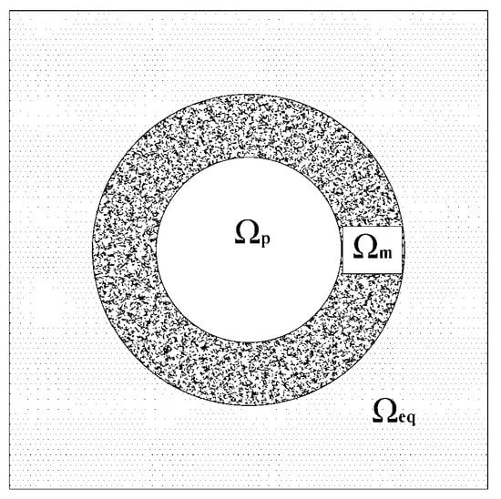
Figure 2.
Calculation model of the solid phase for one-layered CGS.
According to the generalized self-consistent model, the effective bulk modulus (Ks) and shear modulus (Gs) can be obtained [19,36].
where Kp and Km, Gp and Gm are the bulk modulus and shear modulus of pebble and sand–clay matrix, p0 is the volume fraction of pebble, A1, B1, C1 are undetermined coefficients.
It is worth mentioning that the pebble is actually an irregular polyhedron rather than the regular sphere. Under the same volume condition, the sphere has the smallest surface area while the tetrahedron (the simplest convex polyhedrons) has the largest surface area. Since the contacted surface area of pebble with sand–clay matrix affects the mechanical properties of the solid phase greatly, the volume of sphere pebble must be increased in order to match the same surface area of the actual irregular convex polyhedron. Define a shape factor ρ to describe the amplification effect of actual polyhedron on the volume fraction of sphere pebble. For the same surface area, the sphere radius of r and the tetrahedron length of l have the relationship as Equation (2):
where ρmax is the maximum value of shape factor ρ.
For the actually irregular convex polyhedron of pebble, ρ = 1–1.8. Substituting ρ into Equation (1) leads to the effective bulk and shear modulus of the solid phase, as Equation (3):
According to Equation (4):
the effective elastic modulus (Es) of the solid phase is shown as Equation (5):
For calculating the effective elastic modulus of the one-layered CGS, gas phase (pore) must be considered. Figure 3 shows the calculation model of the one-layered CGS, i.e., the hollow sphere model, where Ωp1 is the region of gas phase (pore) as inclusion, Ωm1 is the region of solid phase (sand–clay–pebble matrix) and Ωeq1 is the region of equivalent media.
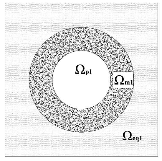
Figure 3.
Calculation model of one-layered CGS.
According to the hollow sphere model, the effective bulk modulus (Ko) and shear modulus (Go) of one-layer CGS with two phases of solid and gas can be obtained [16,36] as Equation (6):
where p1 is pore volume fraction, A2, B2, C2 are undetermined coefficients.
Similarly, the elastic modulus (Eo) is shown as Equation (7).
According to elastic–viscoelastic corresponding principle (the boundary value problem of linear viscoelastic body has the same solution form as that of elastic body in the Laplace space. Therefore, the viscoelastic problem is firstly transformed into Laplace space to calculate its elastic solution and then inversely transformed into Euler space to determine its viscoelastic parameters) [37,38], the viscoelastic parameter of one-layered CGS can be obtained as Equation (8).
where the superscript T means Laplace transform, s is the Laplace transform parameter.
The viscoelastic parameter of one-layered CGS is shown as Equation (9):
2.3. Viscoelastic Parameter Model of the Interface-Layer
Figure 4 shows the calculation model of the interface-layer, where Ωp2 is the region of gas phase (pore) as inclusion, Ωm2 and Ωm3 are the regions of two-layer solid phases and Ωeq2 is the region of equivalent media. Since Ωm2 and Ωm3 are known from the above calculation (Equations (3)–(5)), the interface-layer model can be equivalent to superposition of the hollow sphere model (Ωp2 + Ωm2) and generalized self-consistent model (Ωm3 + Ωp2 + Ωm2).
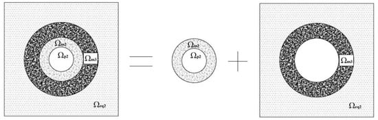
Figure 4.
Calculation model of interface-layer.
According to the hollow sphere model, the equivalent bulk modulus (Ke) and shear modulus (Ge) of Ωp2 − Ωm2 region can be obtained as Equation (10):
where Ke and Ge are the one-layered CGS effective bulk modulus and shear modulus, p2 is the volume fraction of Ωp2 − Ωm2 region, A3, B3, C3 are undetermined coefficients.
According to the generalized self-consistent model, the equivalent bulk modulus (Ki) and shear modulus (Gi) of interface-layer ((Ωp2 + Ωm2) − Ωm3 region) can be calculated as Equation (11):
where p3 is the volume fraction of pore and A4, B4, C4 are undetermined coefficients.
Similarly, effective elastic parameters of the interfacial layer (Ei) is shown as Equation (12):
Similarly, the viscoelastic parameter (Ji) in Laplace space is shown as Equation (13):
The viscoelastic parameter of interface-layer is shown as Equation (14):
2.4. Viscoelastic Parameter Formulae of the Multi-Layered CGS
Since the multi-layered CGS consists of several one-layered CGS and interface-layers, its elastic modulus (E) can be obtained by the series formula as Equation (15):
where Eu, Ei, El are the elastic modulus of the upper layer, interface-layer, and lower layer, respectively.
According to the elastic–viscoelastic corresponding principle, there is the relationship between the elastic parameters (ET) and viscoelastic parameters (JT) (Equation (16)) in the Laplace space:
For determination of the viscoelastic parameters J in Euler space, ET is firstly calculated by the Laplace transform of E (Equation (15)) and then JT is obtained by Equation (16). Finally, J can be calculated by the inverse Laplace transform of JT, as Equation (17):
3. Viscoelastic Parameter Prediction of the Multi-Layered CGS
3.1. Measuring Viscoelastic Parameters of the Sand–Clay Matrix
According to the Code for Design on Subgrade of Railway in China, TB10001-2005 [39], three different mass ratios of sand to clay (Table 1) were selected and uniformly mixed for preparation of the cylindric specimens (Φ 300 mm × 600 mm) by layered compacting method (Figure 5). Triaxial creep tests were conducted by TAJ-2000 triaxial testing system (Figure 6), where the axial stress σ1 was 300 kPa and confining pressure σ3 was 200 kPa (σ3 < σ1).

Table 1.
Mass ratios of sand–clay matrix.
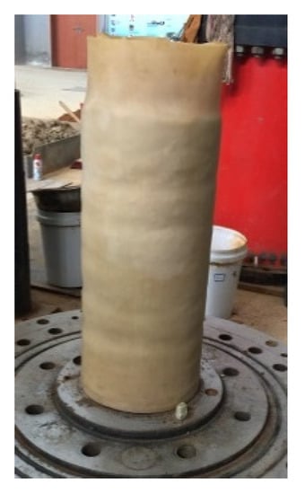
Figure 5.
Sand–clay matrix specimen.
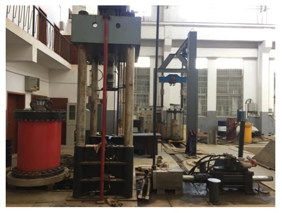
Figure 6.
TAJ-2000 triaxial testing system.
Figure 7 shows the tested creep curves of different sand–clay matrices. They are all composed of three stages: instantaneous deformation (t = 0) stage, attenuation deformation stage (slope is decreased) and stable creep deformation stage (slope is constant). The higher the clay content, the larger the instantaneous deformation and the longer the duration time of the attenuation deformation stage. The clay content has a smaller effect on the stable creep deformation rate, since the elastic properties of the sand–clay matrices are mainly decided by the sand content and the viscous properties by clay content, that is, the viscous properties will play a dominant role as time continues, especially after the attenuation deformation stage, so the creep curves have an almost identical slope on stable creep deformation for viscosity of clay.
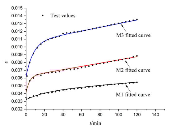
Figure 7.
Fitted curves and test values of different sand–clay matrices.
Burgers rheological model is usually adopted to describe the creep curve as Equation (18):
where Jm is the parameter of Burgers model, E1 and E2 are elastic parameters, η1 and η2 are the viscosity parameters, t is time.
Table 2 lists the fitting viscoelastic parameters of different sand–clay matrices by the Burgers rheological model with high precision (R2 > 0.98). They are all decreased as the clay content increases, indicating that the viscoelastic properties of the sand–clay matrices mainly depend on the clay contents.
Table 2.
Viscoelastic parameters of sand–clay matrix (σ1 − σ3 = 100 kPa).
3.2. Predicting Viscoelastic Parameters of Multi-Layered CGS
In the multi-layered CGS, the pebble and the sand–clay matrix are regarded as elastic and viscoelastic material, respectively. They are exploited from the local area, with the elastic modulus of pebble (Ep = 50 GPa) and density is 2.54 g/cm3, and Poisson’s ratio of pebble (νp = 0.25) and sand–clay matrix (νm = 0.25). Assuming the volume fraction of pore (p1) is 20% [40], the volume fraction of pebble (p0) and sand–clay matrix (p3) can be calculated by the mass-density formula.
Multi-layered CGS consists of several one-layered CGS and interface-layers (Figure 1). The volume fraction of one-layered CGS and the basic parameters of each component are in Table 3.
Table 3.
Basic parameters of one-layered CGS.
Based on Table 3, viscoelastic parameters (ρ = 1) of the multi-layered CGS can be calculated by the following steps:
- Calculate the elastic modulus (ET, superscript T means Laplace space) of the sand–clay matrix by the elastic–viscoelastic correspondence principle as Equation (19).where s is Laplace transform parameter.
- Calculate the equivalent elastic modulus (Ks, Es) of the solid phase (pebble, sand–clay matrix) by Equations (1) and (4).
- Calculate the equivalent elastic modulus (Ko, Eo) of the one-layered CGS by Equations (6) and (7).
- Calculate the equivalent elastic modulus (Ki, Ei) of the interface-layers by Equations (10)–(12).
- Calculate the equivalent elastic modulus (E) of the multi-layered CGS by Equation (15).
- Calculate the equivalent viscoelastic parameters (J) of the multi-layered CGS by Equation (16). and elastic–viscoelastic correspondence principle, as listed in Table 4.
Table 4. Predicted viscoelastic parameters of multi-layered CGS.
4. Experimental Verification
Triaxial creep tests were conducted to verify the viscoelastic parameters of multi-layered CGS (Table 4), since the predicted creep curves could be calculated by the predicted viscoelastic parameters of multi-layered CGS for comparison of test results.
Take three-layered CGS as an example and assume that each single layer has the same heights (H) and each interface-layer (height h1 and h2) has the same proportional height (0.5 h1 or 0.5 h2) in upper and lower layers (Figure 1). Therefore, the actual heights of the top and bottom layers are H′ = H − 0.5 h1 and H − 0.5 h2 and the middle layer is H′′ = H − 0.5h1 − 0.5h2.
The total creep stain (ε) is equal to Equation (20)
where εl1, εi1/2, εl2, εi2/3, εl3 and ul1, ui1/2, ul2, ui2/3, ul3 are creep strain and deformation of the layer 1, interface-layer 1/2, layer 2, interface-layer 2/3 and layer 3, respectively. Jl1, Ji1/2, Jl2, Ji2/3, Jl3 are viscoelastic parameters of the layer 1, interface-layer1/2, layer 2, interface-layer2/3 and layer 3, respectively.
4.1. Triaxial Creep Test
Cylindric specimen of Φ 300 mm × 600 mm in size was adopted in the triaxial creep test. Heights of each layer were 300 mm for two-layered CGS and 200 mm for three-layered CGS. For preparation of one-layered CGS specimen, the pebble was added into the sand–clay matrix (Table 3) to uniformly mixed together by layered compacting method. Table 3 and Figure 8 show their volume fraction and tested gradation curves of pebble, sand, and clay. One-layered, two-layered, and three-layered CGS specimens were tested and their layer combinations were listed in Table 4.
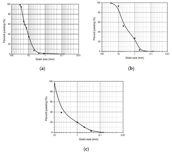
Figure 8.
Gradation curves. (a) pebble; (b) sand; (c) clay.
Similar to Section 3.1, TAJ-2000 triaxial testing system was used in triaxial creep test. The axial stress σ1 was 300kPa and confining pressure σ3 was 200 kPa. Figure 9 shows some specimens after step loading (last step stress is σ1 = 500 kPa) creep tests.
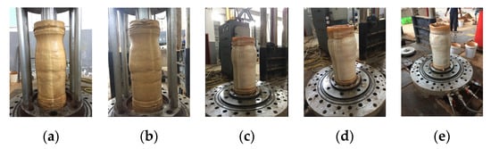
Figure 9.
Deformations of CGS specimens after creep test. (a) L1, (b) L1 + L2, (c) L2 + L3, (d) L1 + L3, (e) L1 + L2 + L3.
4.2. Test Results and Analyses
4.2.1. Creep Curve of One-Layered CGS
Figure 10 shows tested creep curves (ε–t curve) of the one-layered CGS as well as their predicted ones with different values of the shape factor ρ (ρ = 1~1.8, Equation (2)) for comparison. It is seen that all of the tested creep curves consist of three stages: instantaneous deformation, attenuation deformation, and stable creep deformation. Obviously, the higher the content (volume fraction) of pebble (L1 > L2 > L3 in Table 4), the smaller the creep deformation of the one-layered CGS (Figure 10a < Figure 10b < Figure 10c).
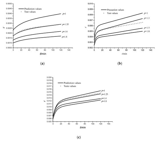
Figure 10.
Tested and predicted creep curves of different one-layered CGS. (a) L1, (b) L2, (c) L3.
It is also found that all of the predicted creep curves of the one-layered CGS decreased with the increase of ρ, since the larger the value of ρ (i.e., the more irregular the shape of pebble), the larger the contacted surface area of pebble with sand–clay matrix and hence the smaller the creep deformation. Furthermore, the predicted curves of ρ = 1 (ideal sphere pebble) are all larger than the tested curves. That is because the actual irregular polyhedron of pebble with a large contacted surface area would lead to small creep deformation.
Comparison of the tested and predicted creep curves of different sand–clay matrix (L1, L2, L3), indicates they are all in good agreement at ρ = 1.35, 1.3, 1.25, respectively. This means the one-layered CGS with a higher content of pebble (L1 > L2 > L3) has a greater possibility of irregular pebble and thus a larger value of ρ.
4.2.2. Viscoelastic Parameter–Time Curves of Interface-Layer
Figure 11 shows viscoelastic parameter–time curves of three one-layered CGS (L1, L2, L3) and their combined interface-layers (L1/L2, L2/L3, L1/L3) which can be drawn by data in Table 4, i.e., J-t curves. Similar to J-t curve of the one-layered CGS, they all consist of three stages: instantaneous deformation, attenuation deformation, and stable creep deformation. The J of the interface-layers (e.g., L1/L2) are between those of the two combined one-layered CGS (e.g., L1 and L2) and smaller than the average values of two one-layered CGS (e.g., (L1 + L2)/2).
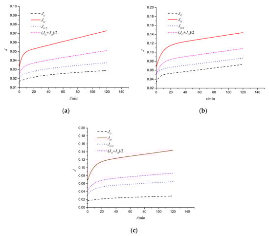
Figure 11.
Viscoelastic parameter–time curves of three one-layered CGS and their combined interface-layers (a) L1, L2, and L1/L2, (b) L2, L3, and L2/L3, (c) L1, L3, and L1/L3.
4.2.3. Creep Curve of Two-Layered CGS
Figure 12 shows the tested creep strains (ε–t) of the two-layered CGS (L1 and L2, L2 and L3, L1 and L3) as well as the predicted ε–t curves with different interface-layer heights, (h = 0~0.5 H, H is the designed height of each layered CGS, H = 300 mm for the two-layered CGS, the total specimen height is 600 mm). They all have the same stages as those of the one-layered CGS: instantaneous deformation, attenuation deformation, and stable creep deformation. In addition, they all decrease as the interface-layer height (h) increases. That is because the interface-layer has a smaller viscoelastic parameter than the average values of the two one-layered CGS, e.g., JL1/L2 < (JL1 + JL2)/2, the total creep strain (ε) is decreased with increase of h according to the following formula (Equation (21)), when H is given. The higher the interface-layer, the weaker the rheological behavior of the two-layered CGS.
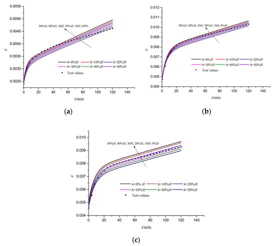
Figure 12.
Tested and predicted creep curves of the two-layered CGS with different interface-layer heights. (a) L1/L2, (b) L2/L3, (c) L1/L3.
It is also found that most of the tested creep strain are between the predicted ε–t curves of 20%H and 30% H, which can prove the existence of the interface-layer and validity of the interface-layer calculation model. The suitable interface-layer height is h = (20–30%)H.
4.2.4. Creep Curve of Three-Layered CGS
Figure 13 shows the tested creep strain of the three-layered CGS (L1, L2 and L3) as well as its predicted ε–t curves with consideration of different interface-layer numbers: N = 1 (L1 + L1/L2 + L2 + L3 or L1 + L2 + L2/L3 + L3) and N = 2 (L1 + L1/L2 + L2 + L2/L3 + L3), where each interface-layer height is h = 0.3 H (H = 200 mm for the three-layered CGS, the total specimen height is 600 mm). Similarly, they all have the same three stages as those both the one-layered and two-layered CGS: instantaneous deformation, attenuation deformation, and stable creep deformation.
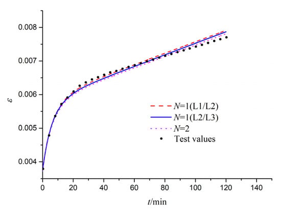
Figure 13.
Tested and predicted creep curves of the three-layered CGS with different interface-layer numbers.
The three-layered CGS has two interface-layers. The more the interface-layers are taken into account in calculation equation (Equation (19)), the predicted creep deformation becomes smaller, since it is known from Section 4.2 that the interface-layer with some height would decrease the deformation of multi-layered CGS, furthermore, three-layered CGS has two interface-layers with the height of 30% H, therefore, two interface-layers has the smallest deformation. The tested results agree well with the predicted results of the three-layered CGS with N = 1 or 2. This proves again the interface-layer really exists in the multi-layered CGS and the established interface-layer calculation model is reasonable and reliable. At least one interface-layer must be considered for predicting viscoelastic parameters of the multi-layered CGS.
4.2.5. Comparing the Creep Curves of Two-Layered and Three-Layered CGS
The above triaxial creep test results of the one-layered, two-layered, and three-layered CGSs have proved the validity of increasing the degree of irregular pebble and height of interface-layer can decrease the creep deformation. For studying the effect of layer number on the creep curve of multi-layered CGS, take two-layered CGS (L1 + L1/L2 + L2 or L2 + L2/L3 + L2) and three-layered (L1 + L1/L2 + L2 + L2/L1 + L1 or L2 + L2/L3 + L3 + L2/L3 + L2) CGS compacted by the same gradation of one-layered CGS (L1 and L2 or L2 and L3) under the same total height (600 mm) for comparison.
Figure 14 shows the predicted creep curves of the two-layered CGS (each layer height H = 300 mm and interface-layer height h = 0.3 H = 90 mm) and three-layered CGS (each layer height H = 200 mm and interface-layer height h = 0.3 H = 60 mm). It is seen that the three-layered CGS has more interface-layer and smaller creep deformation than the two-layered CGS, since the existence of interface-layer decreases the creep deformation (Figure 12). The more the interface-layer, the larger the total height of the interface-layer and thus the smaller the creep deformation. Obviously, the multi-layered CGS of more layer numbers can reduce settlement but also cause difficulty in field compaction and high cost. Both safety and economy must be considered in the design of a pavement or embankment.
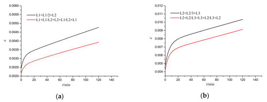
Figure 14.
Predicted creep curves of the two-layered and three-layered CGS compacted by the same gradations of single layer. (a) L1 and L2, (b) L2 and L3.
5. Conclusions
- (1)
- The interface-layer of viscoelasticity and the actual shape of large-particle inclusion were firstly considered and a new interface-layer method was proposed to predict viscoelastic parameters of multi-layered CGS based on homogenization method and elastic–viscoelastic corresponding principle. The tested creep curves of the multi-layered CGS agreed well with the predicted ones and can prove the existence of the interface-layer and verify the validity of this new method.
- (2)
- For the one-layered CGS, the creep deformation decreased as the shape factor (ρ) of pebble inclusion increased and ρ was in the range of 1–1.8.
- (3)
- The viscoelastic parameters of the interface-layer were smaller than the average values of one-layered CGS which consisted of the interface-layer.
- (4)
- For the two-layered CGS, the creep deformation decreased with the increase of the interface-layer height (h) and the suitable interface-layer height was 20–30% as much as the height of one-layered CGS.
- (5)
- For the three-layered CGS, the creep deformation decreased with the increase of the interface-layer number (N) and at least one interface-layer must be taken into account.
- (6)
- For the safety point of view, it is better to use a high degree of irregular pebble and a large difference in gradation of CGS and more layer numbers to reduce the creep deformation of multi-layered coarse-grained soil. Construction costs should be taken into account in design of pavement or embankment.
Author Contributions
Conceptualization, J.Z. and Q.R.; data curation, J.Z.; funding acquisition, Q.R.; methodology, J.Z. and W.Y.; project administration, Q.R.; supervision, Q.R. and W.Y.; validation, J.Z. and Q.R.; writing—original draft, J.Z.; writing—review and editing, Q.R., and W.Y. All authors have read and agreed to the published version of the manuscript.
Funding
National Natural Science Foundation of China under Grant number 51274251.
Acknowledgments
The authors sincerely thank the support of the above fund project and the help of leaders and operators of the test site. Without these supports, the data and field test required by this research would not be able to completed.
Conflicts of Interest
The authors declare no conflict of interest.
References
- Ministry of Water Resources of the People’s Republic of China. GB/T 50145—2007. Standard for Engineering Classification of Soil; Planning Press: Beijing, China, 2008; pp. 94–96.
- Medley, E. The Engineering Characterization of Mélanges and Similar Block-In-Matrix Rocks (Bimrocks). Ph.D. Thesis, University of California, California, CA, USA, 1994. [Google Scholar]
- Wang, T.; Liu, S.; Feng, Y.; Yu, J. Compaction Characteristics and Minimum Void Ratio Prediction Model for Gap-Graded Soil-Rock Mixture. Appl. Sci. 2018, 8, 2584. [Google Scholar] [CrossRef]
- Guo, G.Q. Engineering Characteristics and Application of Coarse Grained Soil; The Yellow River Water Conservancy Press: Zheng Zhou, China, 1998. [Google Scholar]
- Chen, J. Study on Mechanism of Effect of Particle Packing Structure on Engineering Properties of Coarse-Grained Soil Filling High-Speed Railway Embankment. Ph.D. Thesis, Southwest Jiaotong University, Guangzhou, China, 2014. [Google Scholar]
- Ministry of Transport of the People’s Republic of China. Technical Specifications for Construction of Highway Subgrade JTG/T 3610-2019; Communications Press: Beijing, China, 2019.
- Ghalesari, A.T.; Rasouli, H. Effect of Gravel Layer on the Behavior of Piled Raft Foundations. ASCE GSP 2014, 240, 373–382. [Google Scholar] [CrossRef]
- Ghalesari, A.T.; Tabari, M.K.; Choobbasti, A.J.; EsmaeilpourShirvanib, N. Behavior of eccentrically loaded shallow foundations resting on composite soils. J. Build Eng. 2019, 23, 220–230. [Google Scholar] [CrossRef]
- Duong, T.V.; Cui, Y.J.; Tang, A.M.; Dupla, J.C.; Canou, J.; Calon, N.; Robinet, A. Investigating the mud pumping and interlayer creation phenomena in railway sub-structure. Eng. Geol. 2014, 171, 45–58. [Google Scholar] [CrossRef]
- Zhang, S.; Li, Y.; Li, J.; Liu, L. Reliability Analysis of Layered Soil Slopes Considering Different Spatial Autocorrelation Structures. Appl. Sci. 2020, 10, 4029. [Google Scholar] [CrossRef]
- Moayedi, H.; Bui, D.T.; Thi Ngo, P.T. Neural Computing Improvement Using Four Metaheuristic Optimizers in Bearing Capacity Analysis of Footings Settled on Two-Layer Soils. Appl. Sci. 2019, 9, 5264. [Google Scholar] [CrossRef]
- Chen, X.B. Research on the Highway Embankment Granular Soil Fillings’ Rheological Properties. Ph.D. Thesis, Central South University, Changsha, China, 2007. [Google Scholar]
- Feng, Y.; Phillion, A.B. A 3D meso-scale solidification model for metallic alloy using a volume average approach. Materialia 2019, 6, 100329. [Google Scholar] [CrossRef]
- Zheng, H.W.; Peng, X.H.; Ding, J.P.; Tian, Z.A. Micromechanical Model of Ceramic Particulate Reinforced Composites. China Ceram. 2016, 52, 39–42. (In Chinese) [Google Scholar]
- Tang, X.W. Study on Damage and Fracture Behavior of Concrete Based on Macro and Meso Mechanics. Ph.D. Thesis, Tsinghua University, Beijing, China, 2008. [Google Scholar]
- Du, X.L.; Jin, L.; Ma, G.W. Macroscopic effective mechanical properties of porous dry concrete. Cem. Concr. Res. 2013, 44, 87–96. [Google Scholar] [CrossRef]
- Chang, D.; Lai, Y.M.; Zhang, M.Y. A meso-macroscopic constitutive model of frozen saline sandy soil based on homogenization theory. Int. J. Mech. Sci. 2019, 159, 246–259. [Google Scholar] [CrossRef]
- Wang, Z.C. Study on Viscoelastic Properties of Asphalt Mixtures Based on Micromechanics. Ph.D. Thesis, Dalian Maritime University, Dalian, China, 2011. [Google Scholar]
- Wang, P.; Liu, E.L.; Zhi, B. A macro–micro viscoelastic-plastic onstitutive model for saturated frozen soil. Mech. Mater. 2020, 147, 103411. [Google Scholar] [CrossRef]
- Vallejo, L.E.; Lobo, G.S. The elastic moduli of clays with dispersed oversized particles. Eng. Geol. 2005, 78, 163–171. [Google Scholar] [CrossRef]
- Yang, H.; Zhou, Z.; Wang, X.C. Elastic modulus calculation model of a soil-rock mixture at normal or freezing temperature based on micromechanics approach. Adv. Mater. Sci. Eng. 2015, 2015, 1–10. [Google Scholar] [CrossRef]
- Hu, M. Numerical Method to Study the Physical and Mechanical Characteristics of Sandy Pebble Soil and the Response Caused by Shield Tunneling. Ph.D. Thesis, South China University of Technology, Guangzhou, China, 2014. [Google Scholar]
- Barbero, M.; Bonini, M.; Borri, B.M. Three-dimensional finite element simulations of compression tests on bimrock. In Proceedings of the 12th International Conference of International Association for Computer Methods and Advances in Geomechanics, Goa, India, 1–6 October 2008; pp. 31–37. [Google Scholar]
- Xu, W.J.; Yue, Z.Q.; Hu, R.L. Study on the mesostructure and mesomechanical characteristics of the soil–rock mixture using digital image processing based finite element method. Int. J. Rock. Mech. Min. 2008, 45, 749–762. [Google Scholar] [CrossRef]
- Li, X.; Liao, Q.L.; He, J.M. In-situ tests and a stochastic structural model of rock and soil aggregate in the three gorges reservoir area. Int. J. Rock. Mech. Min. 2004, 41, 702–707. [Google Scholar] [CrossRef]
- Li, C.S.; Ellyin, F.; Wharmby, A. A damage meso-mechanical approach to fatigue failure prediction of cross-ply laminate composites. Int. J. Fatigue 2002, 24, 429–435. [Google Scholar] [CrossRef]
- Rashtiyani, H.A.; Hosseini-Toudeshky, H.; Mondal, M. Analytical study of transverse cracking in cross-ply laminates under combined loading based on a new coupled micro-meso approach. Mech. Mater. 2019, 139, 103149. [Google Scholar] [CrossRef]
- Bedzra, R.; Reese, S.; Simon, J.W. Hierarchical multi-scale modelling of flax fibre/epoxy composite by means of general anisotropic viscoelastic-viscoplastic constitutive models: Part II—Mesomechanical model. Int. J. Solids Struct. 2020, 202, 299–318. [Google Scholar] [CrossRef]
- Liu, X.Y.; Liu, E.L.; Zhang, D.; Zhang, G. Study on effect of coarse-grained content on the echanical properties of frozen mixed soils. Cold Reg. Sci. Technol. 2019, 158, 237–251. [Google Scholar] [CrossRef]
- Tabari, M.K.; Ghalesari, A.T.; Choobbasti, A.J.; Afzalirad, M. Large-Scale Experimental Investigation of Strength Properties of Composite Clay. Geotech. Geol. Eng. 2019, 37, 5061–5075. [Google Scholar] [CrossRef]
- Zhang, H.Y.; Xu, W.J.; Yu, Y.Z. Triaxial testsofsoil–rock mixtures with different rock block distributions. Soils Found 2016, 56, 44–56. [Google Scholar] [CrossRef]
- Mohammad, A.; Parviz, M. Failure patterns of geomaterials with block-in-matrix texture: Experimental and numerical evaluation. ARAB J. Geosci. 2014, 7, 2781–2792. [Google Scholar] [CrossRef]
- Hamidi, A.; Salimi, N.; Yazdanjou, V. Shape and size effects of gravel particles on shear strength characteristics of sandy soils. Geoscience 2011, 20, 189–196. [Google Scholar]
- Kouakou, N.M.; Cuisinier, O.; Masrouri, F. Estimation of the shear strength of coarse-grained soils with fine particles. Transp. Geotech. 2020, 25, 100407. [Google Scholar] [CrossRef]
- Hou, F.; Lai, Y.M.; Liu, E.L. A creep constitutive model for frozen soils with different contents of coarse Grains. Cold Reg. Sci. Technol. 2018, 145, 119–126. [Google Scholar] [CrossRef]
- Zhang, Y.; Han, L. Foundation of Mesomechanics; Science Press: Nanjing, China, 2014. [Google Scholar]
- Kovarik, V. Distributional Concept of the Elastic-Viscoelastic Correspondence Principle. J. Appl. Mech. 1995, 62, 847. [Google Scholar] [CrossRef]
- Park, S.W.; Kim, Y.R.; Schapery, R.A. A viscoelastic continuum damage model and its application to uniaxial behavior of asphalt concrete. Mech. Mater. 1996, 24, 241–255. [Google Scholar] [CrossRef]
- Ministry of Railways of the People’s Republic of China. Code for Design on Subgrade of Railway TB10001-2005; Railway Publishing House: Beijing, China, 2005.
- Ding, Y.; Rao, Y.K.; Ni, Q. Effects of gradation and void ratio on the coefficient of permeability of coarse-grained soil. Hydrogeol. Loeng. Geo. 2019, 46, 108–116. (In Chinese) [Google Scholar]


Publisher’s Note: MDPI stays neutral with regard to jurisdictional claims in published maps and institutional affiliations. |
© 2020 by the authors. Licensee MDPI, Basel, Switzerland. This article is an open access article distributed under the terms and conditions of the Creative Commons Attribution (CC BY) license (http://creativecommons.org/licenses/by/4.0/).