
Identification of Pre-Tightening Torque Dependent Parameters for Empirical Modeling of Bolted Joints


Abstract
:1. Introduction
2. Basic Theory
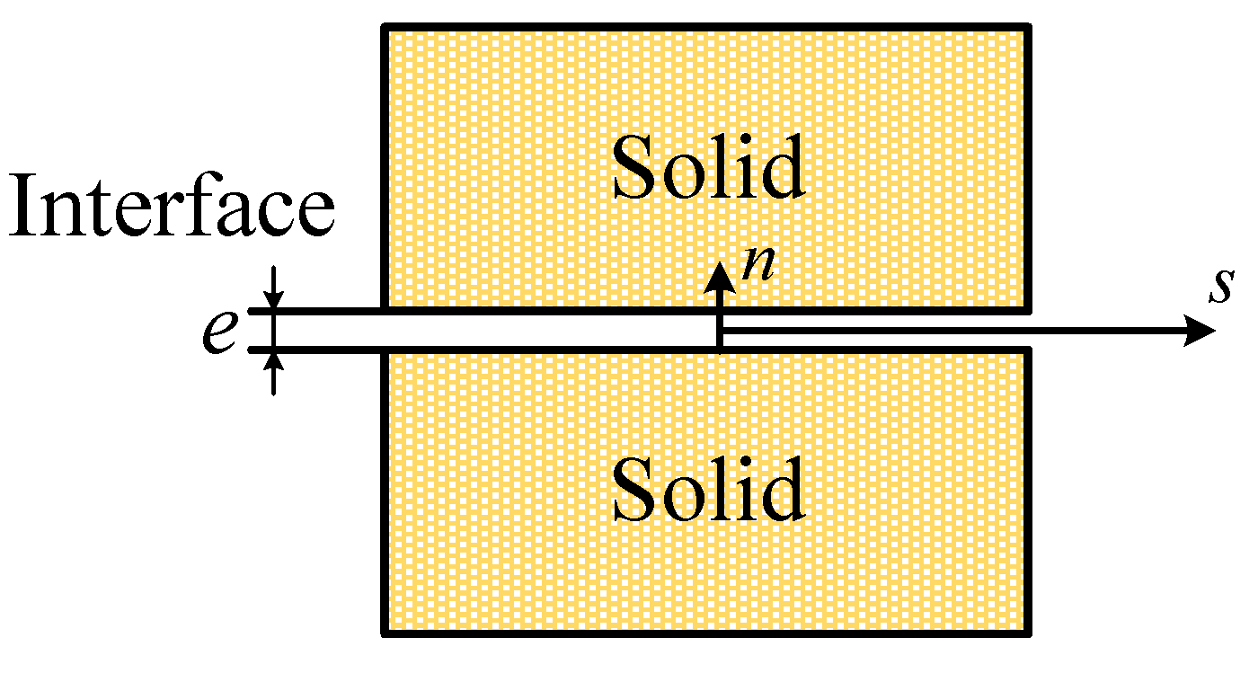
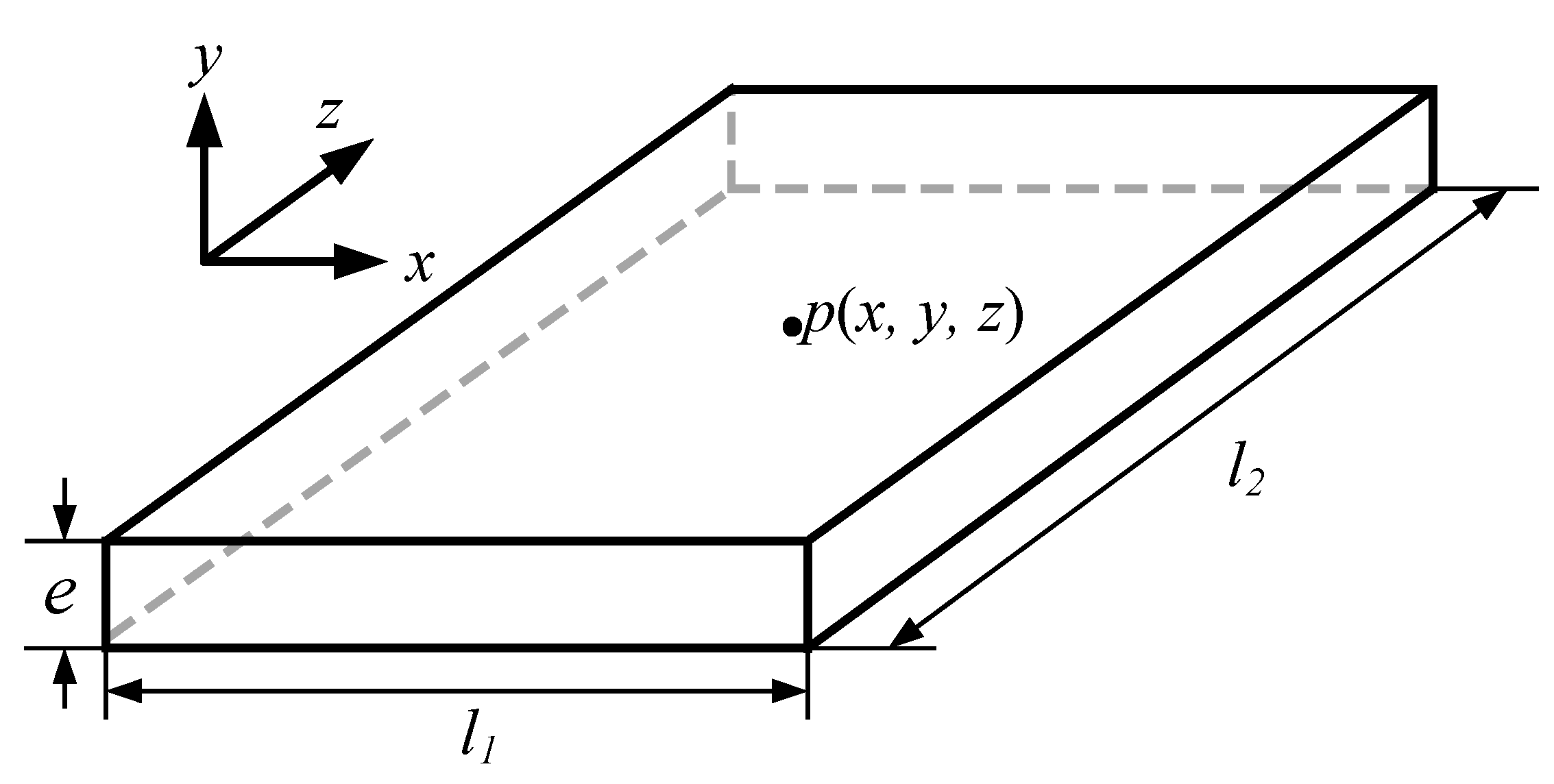
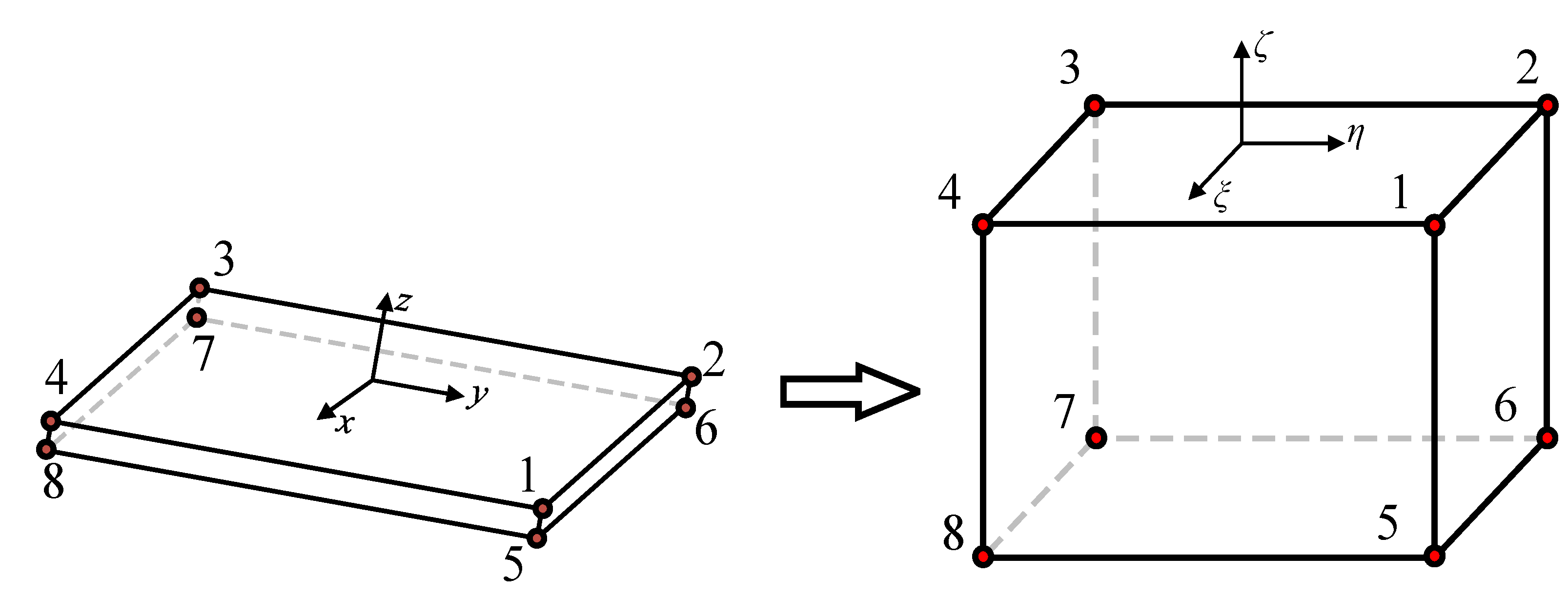
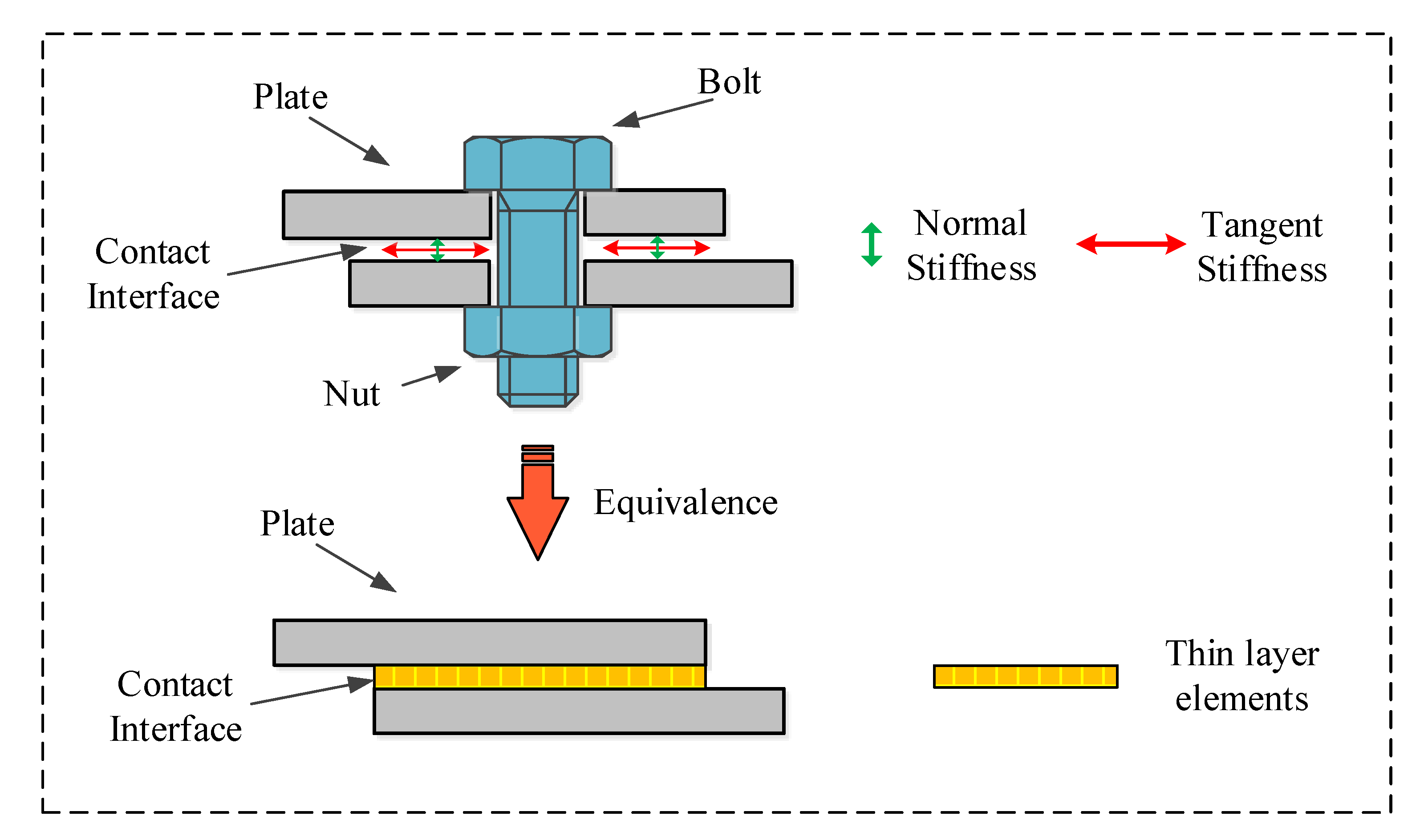
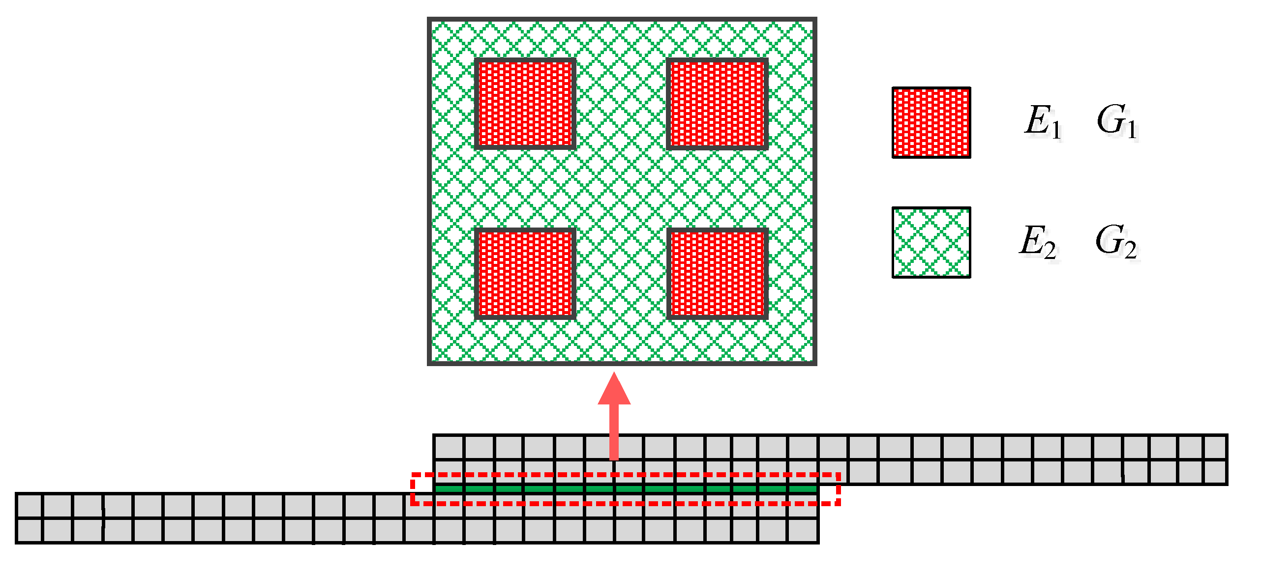
2.1. Thin-Layer Element
2.2. Parameter Identification
- (1)
- Initialize j = 0, construct an initial FE model of the bolt connection using the thin-layer element;
- (2)
- Select the elastic parameters p through relative sensitivity analysis using the initial FE model;
- (3)
- Pair the experimental and numerical modal shapes using modal correlation analysis, calculating the modal assurance criterion (MAC) to achieve this;
- (4)
- Calculate the residual zm − zaj between the experimental and numerical modal data, solve the iteration format Equation (18), and obtain the variation Δp = pj+1 − pj;
- (5)
- If the variables Δp are converged, go to step (6); otherwise set j = j + 1 and go to step (2), with the stop criterion ;
- (6)
- The exact elastic parameters are obtained.
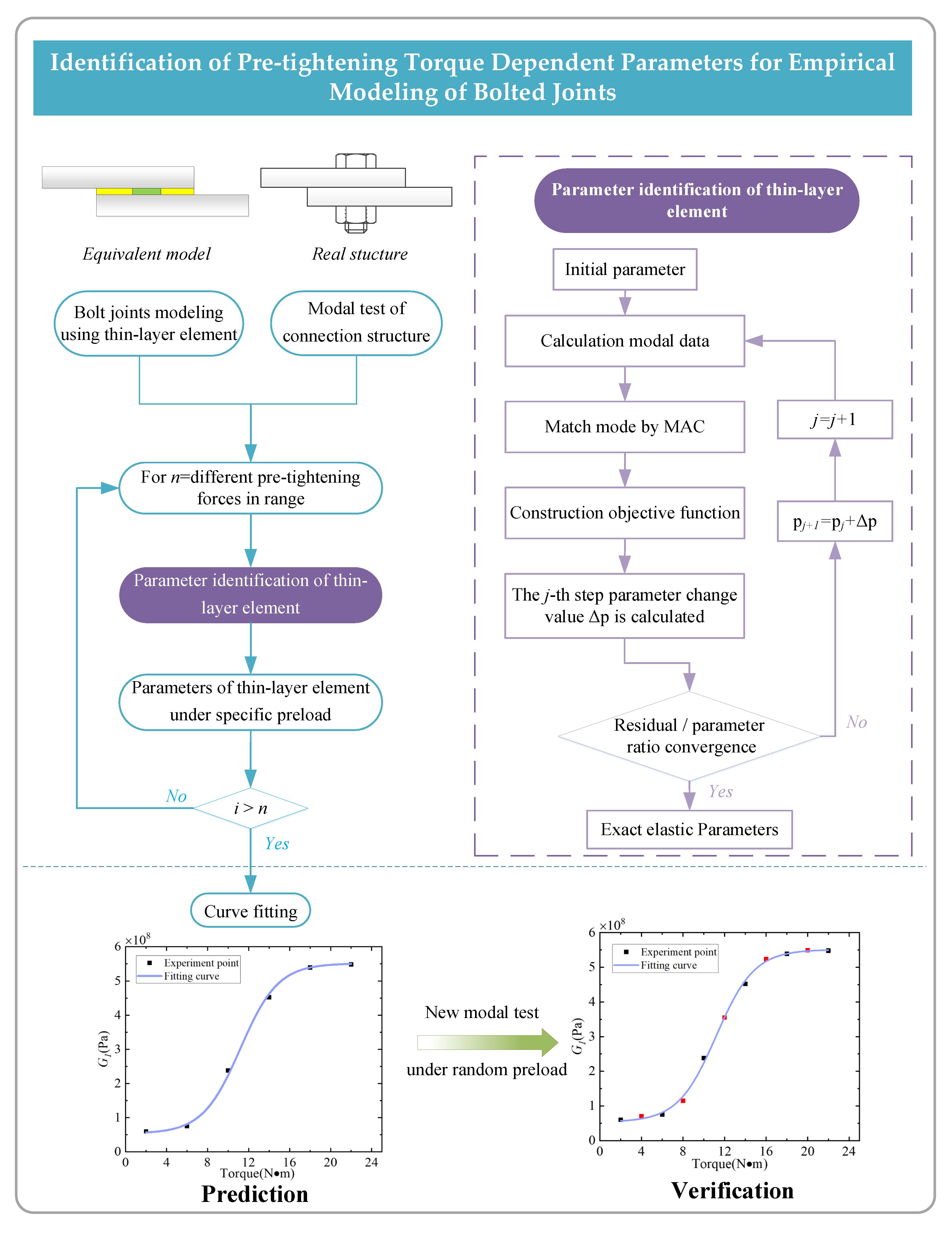
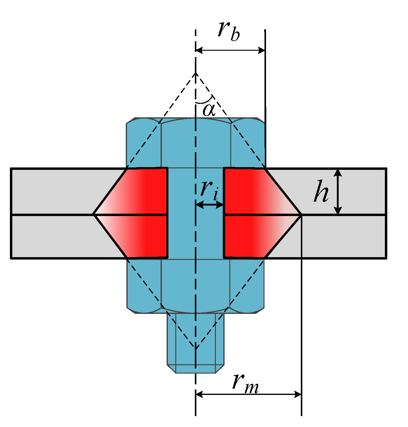
2.3. Pre-Tightening Torque Dependent Parameters
- (1)
- Modelling. The interface of the bolted joint is characterized by the isotropic thin layer element, ignoring the influence of the bolt.
- (2)
- Experiment. The torque wrench is used to get modal data under different pre-tightening torque within a range.
- (3)
- Identification. Under each pre-tightening force, different parameters of the thin layer unit can be obtained through parameter identification, and the precise thin layer element under this pre-tightening force can be obtained.
- (4)
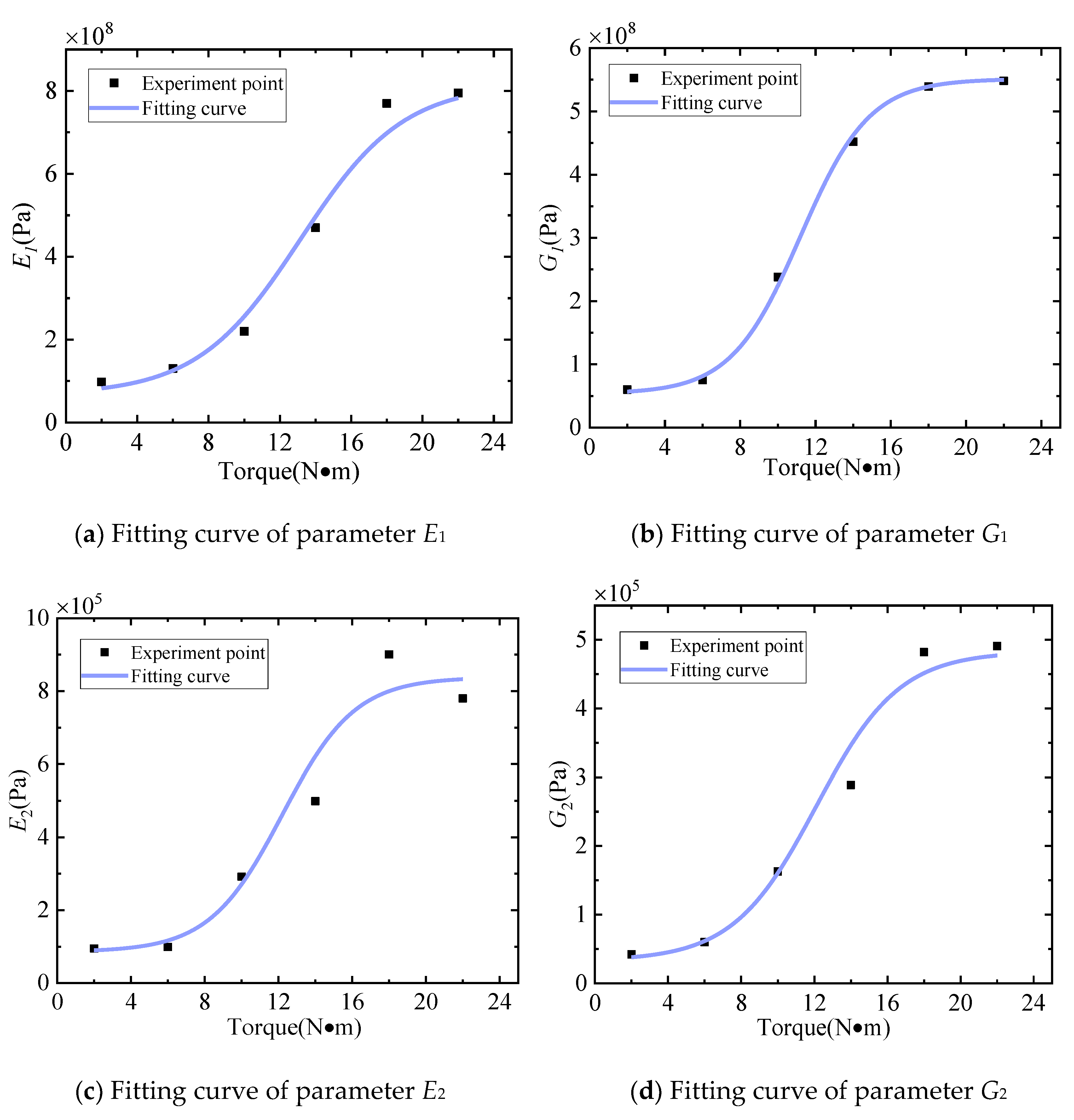
- Prediction. All parameter values of thin-layer elements within a certain range of pre-tightening can be predicted by taking appropriate pre-tightening step and curve fitting.
- (5)
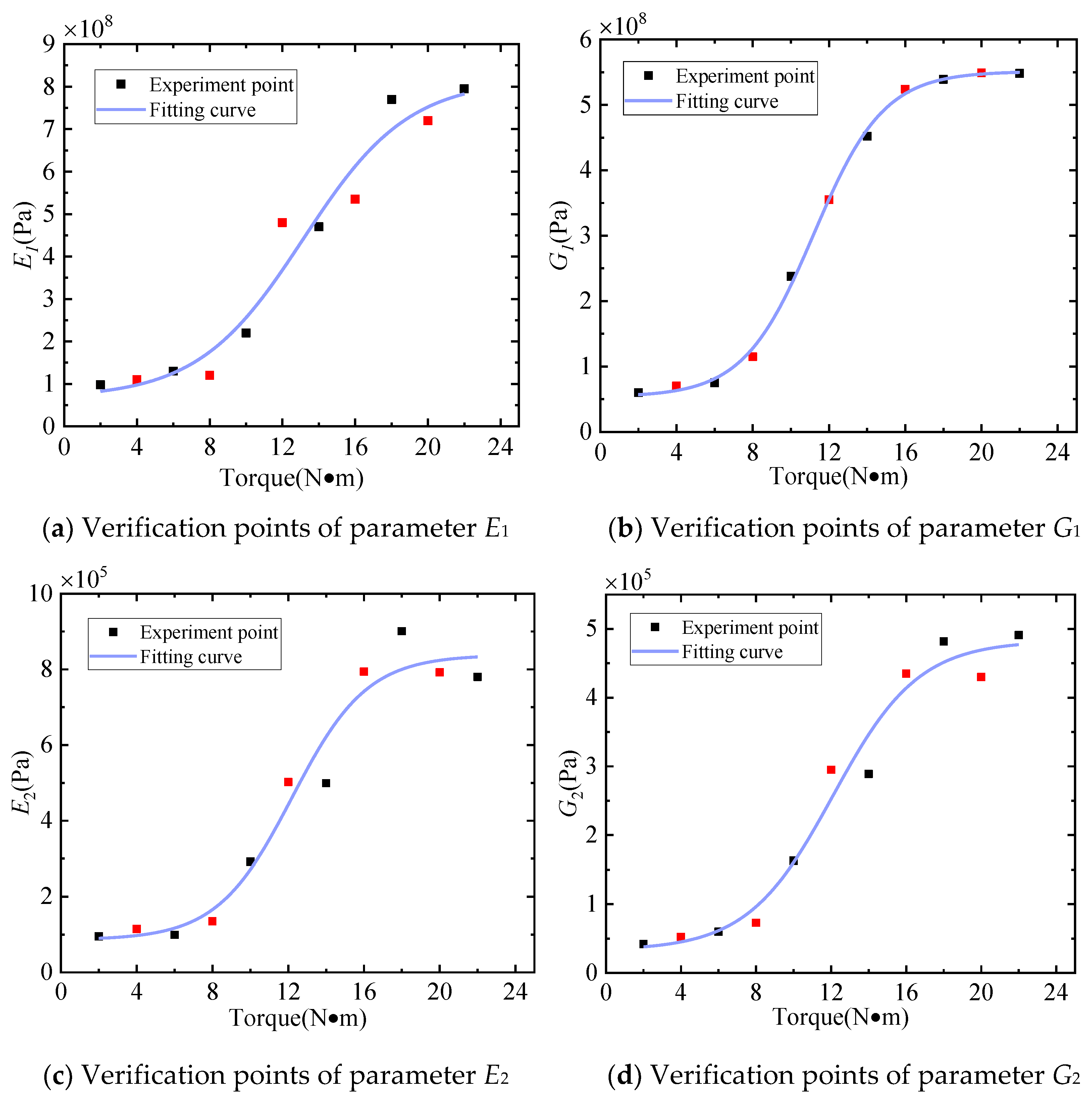
- Verification. New experimental data are used to verify the predictions.
- (6)
- The flowchart of this article is shown in Figure 4.
3. Case Study
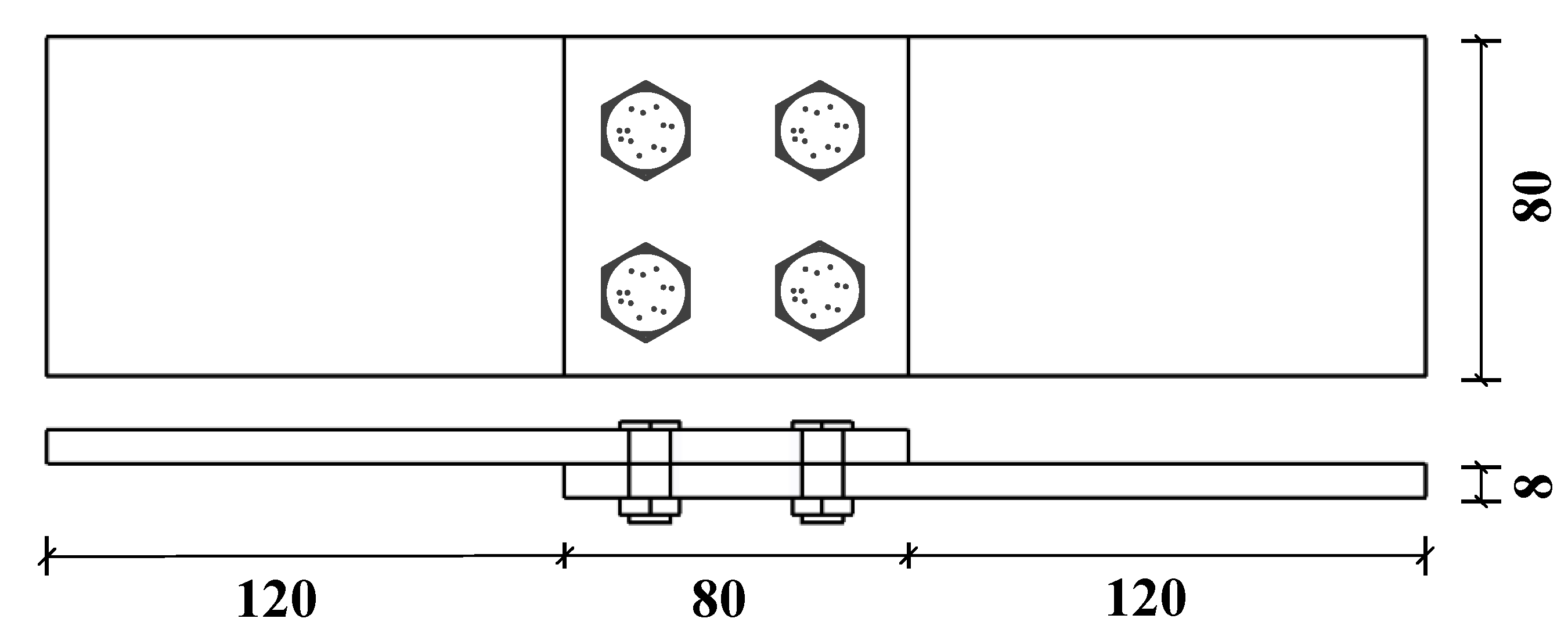
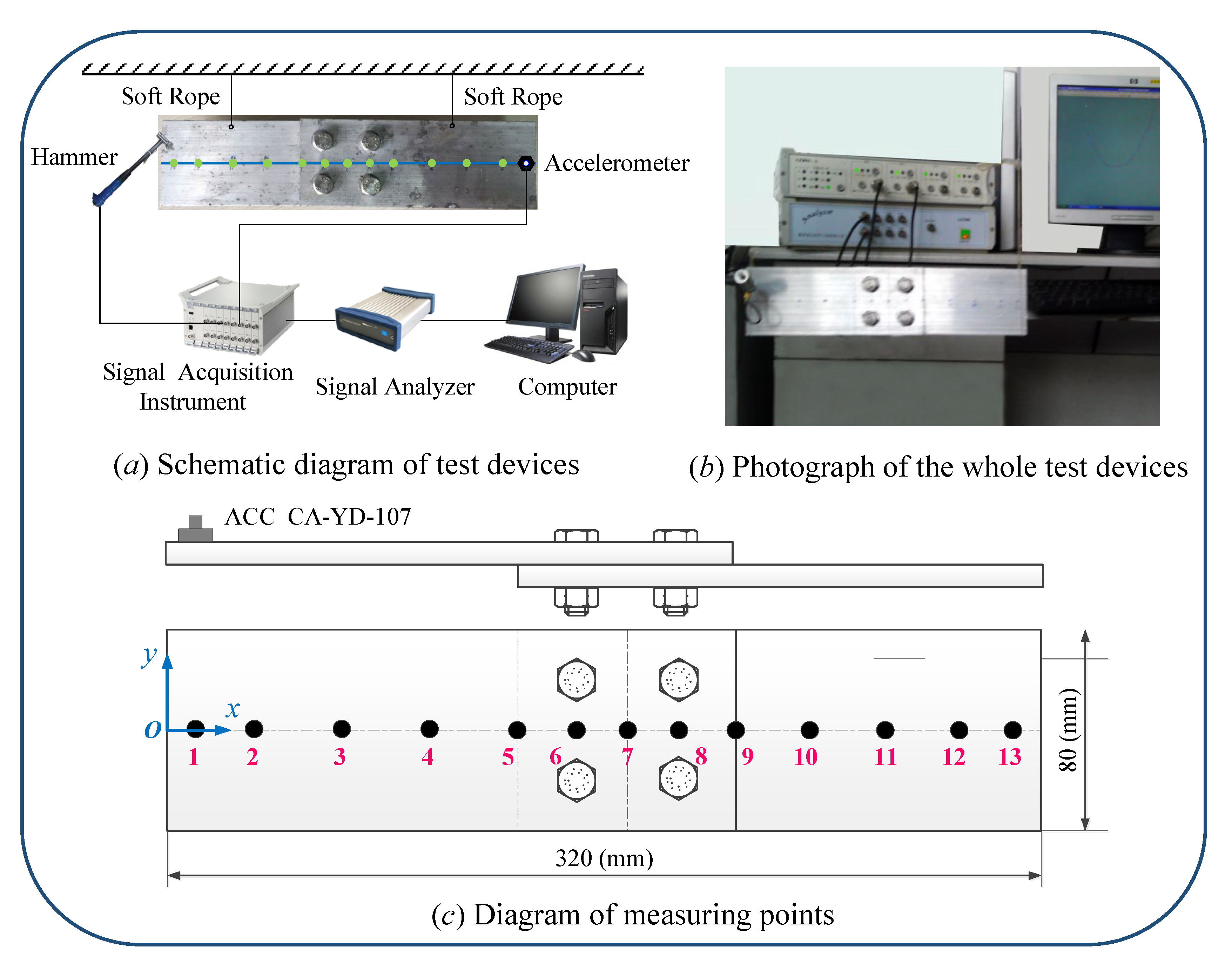
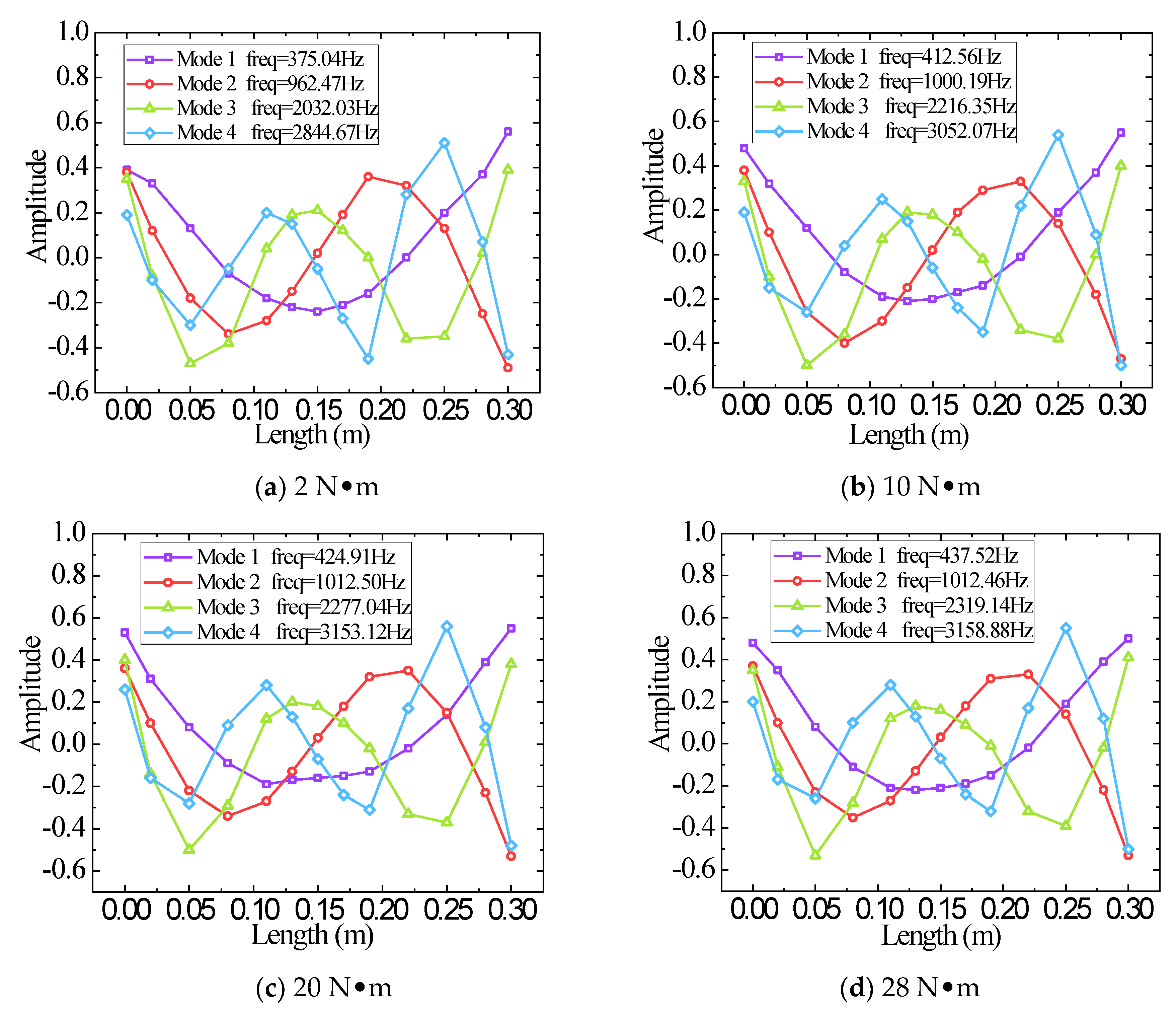
3.1. Modal Test
3.2. Modelling and Parameter Identification
4. Conclusions
- (1)
- Through curve fitting after the parameter identification, the relationship between the pre-tightening torque and the identification parameters can be obtained, which can guide accurate modeling of the same type of bolt connection.
- (2)
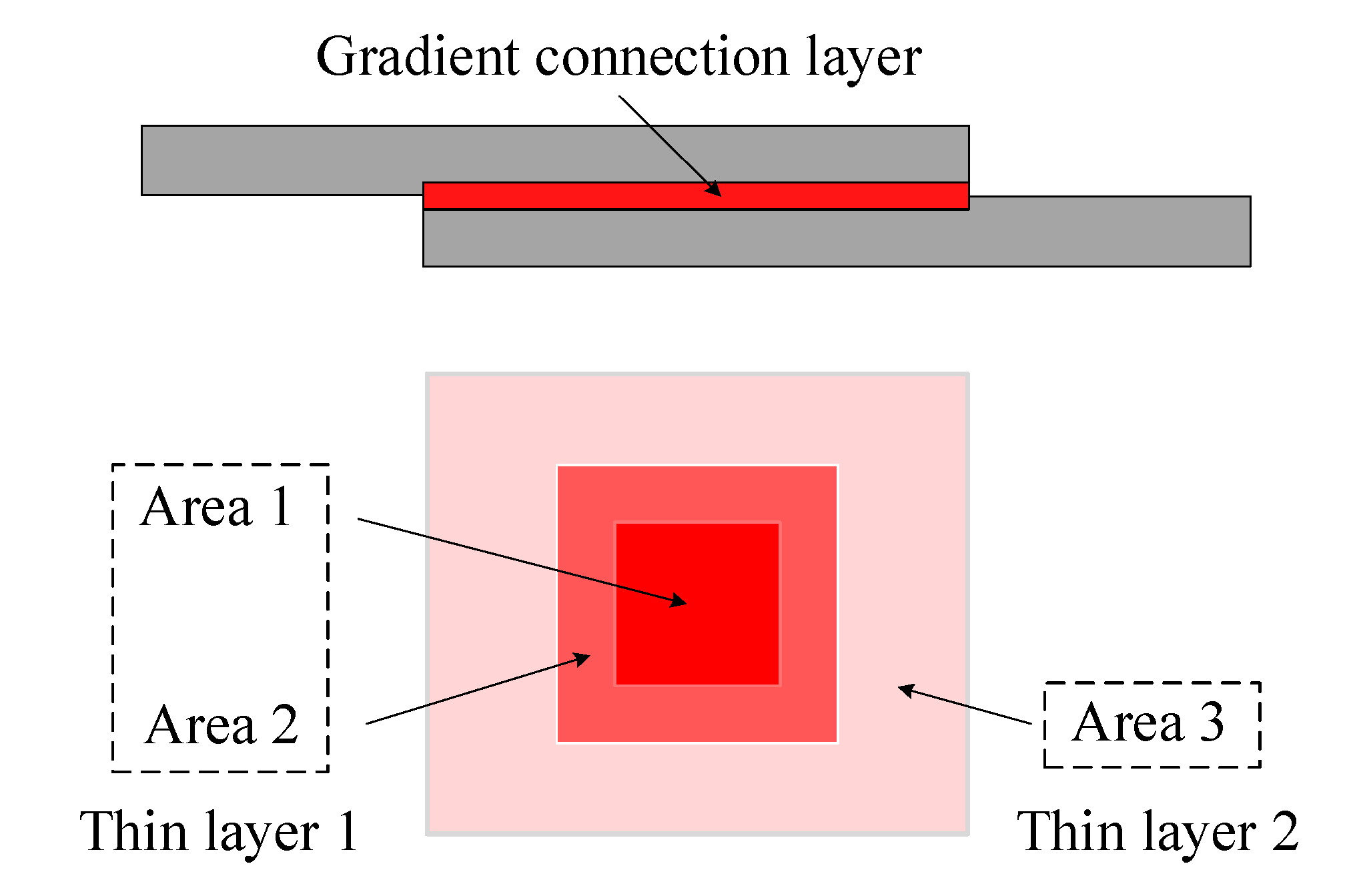
- The thin element method with linear constitutive relation makes modeling and parameter identification very efficient. It can also accurately reflect the contact performance of the joint structure of the bolt lap joint. The identification results for the contact surface material near the bolt area are far greater than for the distance away from the bolt area, which better reflects the inhomogeneity of the contact interface stiffness distribution.
- (3)
- This method can accurately describe the mechanical properties of the contact surface of the bolt lap structure and guide numerical analysis of the bolt connection structure, which has great engineering significance.
Author Contributions
Funding
Institutional Review Board Statement
Informed Consent Statement
Data Availability Statement
Acknowledgments
Conflicts of Interest
References
- Farhad, M.; Majid, M.; Aref, A. Nonlinear behavior of single bolted flange joints: A novel analytical model. Eng. Struct. 2018, 173, 908–917. [Google Scholar] [CrossRef]
- Bograd, S.; Reuss, P.; Schmidt, A.; Gaul, L.; Mayer, M. Modeling the dynamics of mechanical joints. Mech. Syst. Signal Process. 2011, 25, 2801–2826. [Google Scholar] [CrossRef]
- Ibrahim, R.A.; Pettit, C.L. Uncertainties and dynamic problems of bolted joints and other fasteners. J. Sound Vib. 2005, 279, 857–936. [Google Scholar] [CrossRef]
- Luan, Y.; Guan, Z.Q.; Cheng, G.D.; Liu, S. A simplified nonlinear dynamic model for the analysis of pipe structures with bolted flange joints. J. Sound Vib. 2012, 331, 325–344. [Google Scholar] [CrossRef]
- Wang, Z.C.; Xin, Y.; Ren, W.X. Nonlinear structural joint model updating based on instantaneous characteristics of dynamic responses. Mech. Syst. Signal Process. 2016, 76–77, 476–496. [Google Scholar] [CrossRef]
- Li, Z.; Soga, K.; Wang, F.; Wright, P.; Tsuno, K. Behaviour of cast-iron tunnel segmental joint from the 3D FE analyses and development of a new bolt-spring model. Tunn. Undergr. Space Technol. 2014, 41, 176–192. [Google Scholar] [CrossRef]
- Vilela, P.M.L.; Carvalho, H.; Grilo, L.F.; Montenegro, P.A.; Calçada, R.B. Unitary model for the analysis of bolted connections using the finite element method. Eng. Fail. Anal. 2019, 104, 308–320. [Google Scholar] [CrossRef]
- Fukuoka, T. Finite Element Analysis of the Mechanical Behavior of Multibolted Joints Subjected to Shear Loads. J. Press. Vessel. Technol. 2018, 140, 051201. [Google Scholar] [CrossRef]
- Yan, A.M.; Wang, X.F.; Yang, H.; Huang, F.L.; Pi, A.G. Research on the Shock Response Characteristics of a Threaded Connection Using the Thin-Layer Element Method. Appl. Sci. 2021, 11, 5611. [Google Scholar] [CrossRef]
- Ahmadian, H.; Jalali, H. Generic element formulation for modelling bolted lap joints. Mech. Syst. Signal Process. 2007, 21, 2318–2334. [Google Scholar] [CrossRef]
- Yao, X.Y.; Wang, J.J.; Zhai, X. Research and application of improved thin-layer element method of aero-engine bolted joints. Proc. Inst. Mech. Eng. Part G J. Aerosp. Eng. 2017, 231, 823–839. [Google Scholar] [CrossRef]
- Cooper, C.; Turvey, G. Effects of joint geometry and bolt torque on the structural performance of single bolt tension joints in pultruded GRP sheet material. Compos. Struct. 1995, 32, 217–226. [Google Scholar] [CrossRef]
- Zhao, Y.S.; Yang, C.; Cai, L.G.; Shi, W.M.; Hong, Y. Stiffness and Damping Model of Bolted Joints with Uneven Surface Contact Pressure Distribution. Stroj. Vestn. J. Mech. Eng. 2016, 62, 665–677. [Google Scholar] [CrossRef] [Green Version]
- Zhao, G.; Xiong, Z.; Xin, J.; Hou, L.; Gao, W. Prediction of contact stiffness in bolted interface with natural frequency experiment and FE analysis. Tribol. Int. 2018, 127, 157–164. [Google Scholar] [CrossRef]
- Yang, K.T.; Park, Y.S. Joint structural parameter identification using a subset of frequency response function measurements. Mech. Syst. Signal Process. 1993, 7, 509–530. [Google Scholar] [CrossRef]
- Jiang, D.; Wu, S.Q.; Shi, Q.F.; Fei, Q.G. Contact interface parameter identification of bolted joint structure with uncertainty using thin layer element method. Eng. Mech. 2015, 32, 220–227. [Google Scholar] [CrossRef]
- Ren, Y.; Beards, C. Identification of joint properties of a structure using FRF data. J. Sound Vib. 1995, 186, 567–587. [Google Scholar] [CrossRef]
- Tsai, J.S.; Chou, Y.F. Modeling of the dynamic characteristics of two-bolt-joints. J. Chin. Inst. Eng. 1988, 11, 235–245. [Google Scholar] [CrossRef]
- Yang, T.; Fan, S.; Lin, C.S. Joint stiffness identification using FRF measurements. Comput. Struct. 2003, 81, 2549–2556. [Google Scholar] [CrossRef]
- Xu, Y.; Cao, Z.; Jiang, D. Boundary condition identification of a clamped honeycomb sandwich panel based on thin-layer element. J. Vibroeng. 2019, 21, 2286–2295. [Google Scholar] [CrossRef]
- Goodman, R.E. A model for the mechanics of jointed rock. J. Soil Mech. Found. Div. 1968, 94, 637–659. [Google Scholar] [CrossRef]
- Sharma, K.G.; Desai, C.S. Analysis and Implementation of Thin-Layer Element for Interfaces and Joints. J. Eng. Mech. 1992, 118, 2442–2462. [Google Scholar] [CrossRef]
- Givoli, D. Finite element modeling of thin layers. CMES Comput. Modeling Eng. Sci. 2004, 5, 497–514. [Google Scholar] [CrossRef]
- Desai, C.; Zaman, M.; Lightner, J.; Siriwardane, H. Thin-layer element for interfaces and joints. Int. J. Numer. Anal. Methods Geomech. 1984, 8, 19–43. [Google Scholar] [CrossRef]
- Schmidt, A.; Bograd, S.; Gaul, L. Measurement of join patch properties and their integration into finite-element calculations of assembled structures. Shock. Vib. 2012, 19, 1125–1133. [Google Scholar] [CrossRef]
- Jiang, D.; Xu, Y.; Zhu, D.; Cao, Z. Temperature-dependent thermo-elastic parameter identification for composites using thermal modal data. Adv. Mech. Eng. 2019, 11, 1687814019884165. [Google Scholar] [CrossRef] [Green Version]
- Wu, Y.; Zhu, R.; Cao, Z.; Liu, Y.; Jiang, D. Model Updating Using Frequency Response Functions Based on Sherman–Morrison Formula. Appl. Sci. 2020, 10, 4985. [Google Scholar] [CrossRef]
- Jiang, D.; Zhang, D.; Fei, Q.; Wu, S. An approach on identification of equivalent properties of honeycomb core using experimental modal data. Finite Elem. Anal. Des. 2014, 90, 84–92. [Google Scholar] [CrossRef]
- Adel, F.; Shokrollahi, S.; Jamal-Omidi, M.; Ahmadian, H. A model updating method for hybrid composite/aluminum bolted joints using modal test data. J. Sound Vib. 2017, 396, 172–185. [Google Scholar] [CrossRef]


| Gaussian Points | l1 × l2 × e = 1 × 1 × 0.1 | l1 × l2 × e = 5 × 5 × 0.1 | ||||
|---|---|---|---|---|---|---|
| ∂Ni/∂x | ∂Ni/∂y | ∂Ni/∂z | ∂Ni/∂x | ∂Ni/∂y | ∂Ni/∂z | |
| i = 1 | −0.16667 | −0.62201 | −1.66667 | −0.03333 | −0.12440 | −1.66667 |
| i = 2 | 0.16667 | −0.16667 | −0.44658 | 0.03333 | −0.03333 | −0.44658 |
| i = 3 | 0.62201 | 0.16667 | −1.16667 | 0.12440 | 0.03333 | −1.66667 |
| i = 4 | −0.62201 | 0.62201 | −6.22008 | −0.12440 | 0.12440 | −6.22008 |
| i = 5 | −0.04466 | −0.16667 | 1.66667 | −0.00893 | −0.03333 | 1.66667 |
| i = 6 | 0.04466 | −0.04466 | 0.44658 | 0.00893 | −0.00893 | 0.44658 |
| i = 7 | 0.16667 | 0.04466 | 1.66667 | 0.03333 | 0.00893 | 1.66667 |
| i = 8 | −0.16667 | 0.16667 | 6.22008 | −0.03333 | 0.03333 | 6.22008 |
| Material | ρ/(kg/m3) | E/(Pa) | G/(Pa) |
|---|---|---|---|
| Aluminum alloy | 2750 | 6.9 × 10¹⁰ | 2.69 × 10¹⁰ |
| Low-carbon steel | 7900 | 2.1 × 10¹¹ | 8.08 × 10¹⁰ |
| Measuring Point | 1 | 2 | 3 | 4 | 5 | 6 | 7 | 8 | 9 | 10 | 11 | 12 | 13 |
|---|---|---|---|---|---|---|---|---|---|---|---|---|---|
| Position (mm) | 1 | 3 | 6 | 9 | 12 | 14 | 16 | 18 | 20 | 23 | 26 | 29 | 31 |
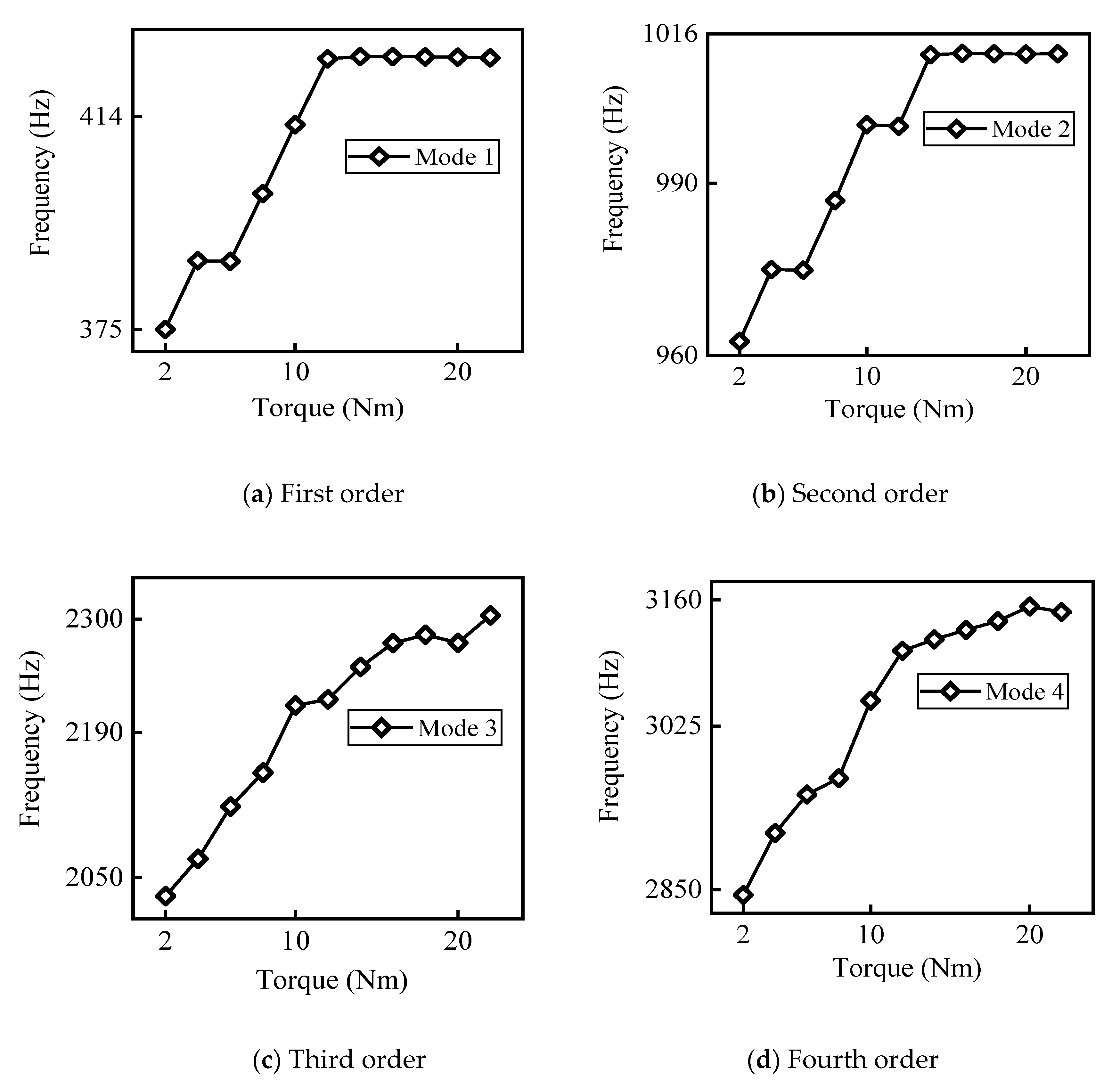
| Pre-Tightening Torque (N·m) | Modal Frequency (Hz) | |||
|---|---|---|---|---|
| Mode 1 | Mode 2 | Mode 3 | Mode 4 | |
| 2 | 375.04 | 962.47 | 2032.03 | 2844.67 |
| 4 | 387.64 | 975.00 | 2068.01 | 2910.88 |
| 6 | 387.50 | 974.89 | 2118.68 | 2952.14 |
| 8 | 399.89 | 986.96 | 2151.37 | 2969.46 |
| 10 | 412.56 | 1000.19 | 2216.35 | 3052.07 |
| 12 | 424.63 | 999.94 | 2222.10 | 3105.54 |
| 14 | 424.99 | 1012.38 | 2253.68 | 3118.02 |
| 16 | 425.00 | 1012.59 | 2276.85 | 3128.10 |
| 18 | 424.96 | 1012.53 | 2284.80 | 3137.43 |
| 20 | 424.91 | 1012.50 | 2277.04 | 3153.12 |
| 22 | 424.80 | 1012.51 | 2303.74 | 3147.28 |
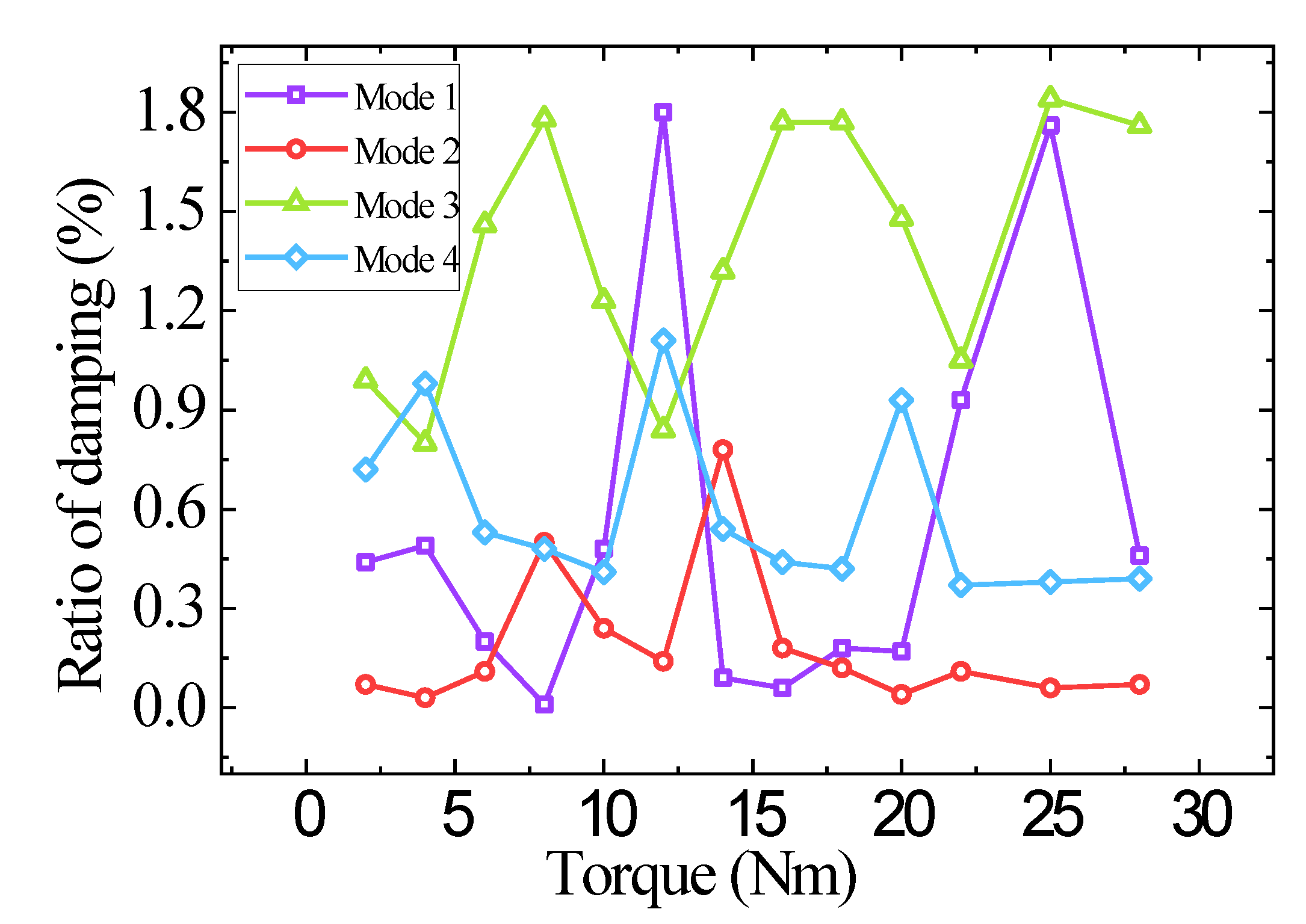
| Pre-Tightening Torque (N·m) | Damping Ratio (%) | |||
|---|---|---|---|---|
| Mode 1 | Mode 2 | Mode 3 | Mode 4 | |
| 2 | 0.44 | 0.07 | 0.99 | 0.72 |
| 4 | 0.49 | 0.03 | 0.80 | 0.98 |
| 6 | 0.20 | 0.11 | 1.46 | 0.53 |
| 8 | 0.01 | 0.50 | 1.78 | 0.48 |
| 10 | 0.48 | 0.24 | 1.23 | 0.41 |
| 12 | 1.80 | 0.14 | 0.84 | 1.11 |
| 14 | 0.09 | 0.78 | 1.32 | 0.54 |
| 16 | 0.06 | 0.18 | 1.77 | 0.44 |
| 18 | 0.18 | 0.12 | 1.77 | 0.42 |
| 20 | 0.17 | 0.04 | 1.48 | 0.93 |
| 22 | 0.93 | 0.11 | 1.05 | 0.37 |
| Identified Parameters (N/m2) | E1 | G1 | E2 | G2 |
|---|---|---|---|---|
| Initial value | 3.00 × 10⁹ | 1.15 × 10⁹ | 3.00 × 10⁶ | 1.15 × 10⁶ |
| Identified value | 8.63 × 10⁸ | 3.42 × 10⁸ | 9.33 × 10⁵ | 4.46 × 10⁵ |
| Order | Experiment (Hz) | Initial (Hz) | Error % | Updated (Hz) | Error % |
|---|---|---|---|---|---|
| 1 | 424.91 | 437.55 | 2.97 | 427.01 | 0.49 |
| 2 | 1012.50 | 1044.80 | 3.19 | 1037.05 | 2.42 |
| 3 | 2277.04 | 2314.00 | 1.62 | 2261.19 | −0.69 |
| 4 | 3153.12 | 3209.10 | 1.78 | 3136.38 | −0.53 |
Publisher’s Note: MDPI stays neutral with regard to jurisdictional claims in published maps and institutional affiliations. |
© 2021 by the authors. Licensee MDPI, Basel, Switzerland. This article is an open access article distributed under the terms and conditions of the Creative Commons Attribution (CC BY) license (https://creativecommons.org/licenses/by/4.0/).
Share and Cite
Tian, Y.; Qian, H.; Cao, Z.; Zhang, D.; Jiang, D. Identification of Pre-Tightening Torque Dependent Parameters for Empirical Modeling of Bolted Joints. Appl. Sci. 2021, 11, 9134. https://doi.org/10.3390/app11199134
Tian Y, Qian H, Cao Z, Zhang D, Jiang D. Identification of Pre-Tightening Torque Dependent Parameters for Empirical Modeling of Bolted Joints. Applied Sciences. 2021; 11(19):9134. https://doi.org/10.3390/app11199134
Chicago/Turabian StyleTian, Yu, Hui Qian, Zhifu Cao, Dahai Zhang, and Dong Jiang. 2021. "Identification of Pre-Tightening Torque Dependent Parameters for Empirical Modeling of Bolted Joints" Applied Sciences 11, no. 19: 9134. https://doi.org/10.3390/app11199134