Article

Development and Validation of Two Intact Lumbar Spine Finite Element Models for In Silico Investigations: Comparison of the Bone Modelling Approaches

1
In Silico Biomechanics Laboratory, National Center for Spinal Disorders, 1126 Budapest, Hungary
2
School of PhD Studies, Semmelweis University, 1085 Budapest, Hungary
3
Department of Orthopaedics, Semmelweis University, 1085 Budapest, Hungary
4
National Center for Spinal Disorders, 1126 Budapest, Hungary
5
Department of Mechatronics, Optics and Mechanical Engineering Informatics, Faculty of Mechanical Engineering, Budapest University of Technology and Economics, 1111 Budapest, Hungary
6
Department of Spine Surgery, Department of Orthopaedics, Semmelweis University, 1085 Budapest, Hungary
*
Author to whom correspondence should be addressed.
These authors contributed equally to this work.
Appl. Sci. 2022, 12(20), 10256; https://doi.org/10.3390/app122010256
Submission received: 15 September 2022 / Revised: 30 September 2022 / Accepted: 9 October 2022 / Published: 12 October 2022
(This article belongs to the Special Issue Medical Imaging: Advanced Techniques and Applications)

Abstract

:
Finite element (FE) analyses contribute to a better understanding of the human lumbar spine’s biomechanics and serve as an effective predictive tool. This study aims to present the development of two L1–L5 FE models using literature-based (LBM) and patient-specific (PSM) bone material assignment approaches. The geometry of the lumbar spine was developed based on quantitative computed tomography scans. The LBM and the PSM were compared under pure and combined loads. Various biomechanical parameters were investigated to validate the models. The total range of motion of the LBM in pure flexion-extension, lateral bending, and axial rotation were 30.9°, 29°, and 13.7°, respectively, while for the PSM, it was 31.6°, 28.6°, and 14.1°. The required computational time of the PSM to complete against pure and combined loads were 12.1 and 16.6 times higher on average compared to the LBM. This study demonstrated that both models agree with experimental and in silico results, although the cumulative distribution of the stress and characterization of strain values showed a noteworthy difference between the two models. Based on these findings, the clinically-focused biomechanical FE studies must perceive the differences in internal mechanical parameters and computational demand between the different bone modelling approaches.

1. Introduction

In recent years, finite element analysis (FEA) has been recognised as an effective predictive tool for assessing spinal biomechanics [1]. The application of FEA can eliminate the difficulties, limitations and ethical concerns associated with in vitro experiments, furthermore, FEA is more cost-effective than in vivo and in vitro experimental studies [2,3]. The possibility of employing complex load cases and boundary conditions allows the investigation of biomechanical parameters that are difficult to measure by experimental methods [4]. Recently, in silico studies and trials using finite element methods are becoming more widespread [5,6,7], enabling patient-specific investigations and the development of new treatments and medical devices [8,9,10].
Numerous validated lumbar spine finite element (FE) models were published in the literature, which have varying degree of patient-specificity depending on the employed modelling strategy [2,11,12]. A commonly used technique is the “hybrid patient-specific” modelling approach, where the geometry is based on the patient’s medical imaging data while the material properties are literature-based [13,14,15]. This approach is frequently employed in various in silico studies, for instance, to determine stress and strain patterns in anatomical components [13], to investigate degenerative lesions [14], to evaluate the effect of surgical procedures [15], or to analyse spinal implants [16]. Shirazi-Adl created an L1–L5 lumbar spine FE model using a 65-year-old male cadaver’s computed tomography (CT) images with material properties taken from the literature to investigate the stress response in soft tissues under various load cases [13]. Park et al. developed an L1-S1 lumbosacral spine FE model utilising the CT scans of a 26-year-old male with literature-based material properties to investigate the biomechanics of disc degeneration [14]. Schmidt et al. created an L1–L5 lumbar spine FE model using the CT scans of a 46-year-old male cadaver, adapting the material properties from the literature to investigate the biomechanical consequences of total disc arthroplasty [15].
Another possible modelling technique is the “fully patient-specific” approach. In this case, both the geometry and bone material properties are defined based on the medical images. Such models can be used to investigate the load-fracture mechanism of bony structures, either with single vertebra models [11,17,18] or motion segments [12,19]. Crawford et al. created a voxel-based vertebral body FE model to investigate vertebral compressive strength with CT-derived bone material properties and geometry [18]. Costa et al. assessed the biomechanical characteristic of vertebrae with lytic lesions using a subject-specific FE model [11]. Xiao et al. developed an FE model of the L4–L5 lumbar motion segment using patient-specific bone material properties to analyse its kinematics by measuring the range of motion (ROM) and comparing it with experimental results [12].
The effects of medical imaging-based bone material properties were evaluated in the literature by comparing their results with simulations employing literature-based material properties. O’Reilly and Whyne compared geometrically parametric models with “fully patient-specific” models to analyse the strain and displacement patterns in healthy and metastatically involved vertebrae in a T6-T8 spinal motion segment. However, only the trabecular bone’s material property was assigned based on the CT scans. They found that both the geometry and material properties have a notable effect on the vertebral strain and displacement [20]. Sapin-de Brosses et al. compared the effect of medical imaging-derived bone material definition with literature-based bone material characteristics using a FEA of fourteen vertebrae. Their study concludes that applying patient-specific bone material properties reduces the relative error of the failure load estimation [21]. As presented, comparative FE studies between patient-specific and literature-based bone material assignment strategies were published in the literature. However, these studies focus mainly on assessing the vertebral strength of the trabecular region and mechanical failure of the bony tissues.
As pointed out, in the field of in silico studies, two main modelling techniques are commonly utilised, the “fully patient-specific” and the “hybrid patient-specific” strategy. Therefore, the current study presents and compares two lumbar spine FE models created according to these modelling strategies. The developed and analysed FE models were the literature-based model (LBM) and the patient-specific model (PSM). Validation was performed using several biomechanical parameters while highlighting these strategies’ specificities, challenges, and limitations. In addition, differences in computational demands and internal mechanical parameters were also assessed.

2. Materials and Methods

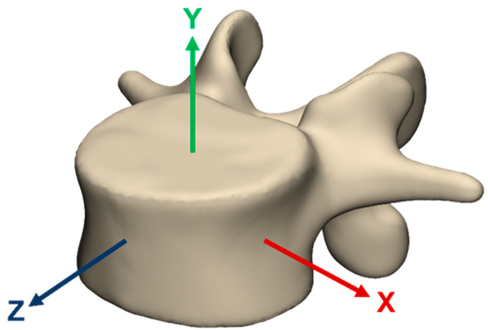
2.1. Geometry of the FE Models

Two finite element models of the intact lumbar spine (L1–L5) were developed using quantitative computed tomography (QCT) images (Hitachi Presto, Hitachi Medical Corporation, Tokyo, Japan) of a 24-year-old male patient without any lumbar spine-related musculoskeletal pathology. The study involving the human participant was reviewed and approved by the National Ethics Committee of Hungary and the National Institute of Pharmacy and Nutrition (reference number: OGYÉI/163-4/2019). Written informed consent was obtained from the individual for the publication of any potentially identifiable images or data included in this article. All methods were carried out in accordance with relevant guidelines and regulations.
The QCT (voxel size of 0.6 × 0.6 × 0.6 mm3) scans were used to obtain the geometry of both FE models, with previously reported imaging protocol [22]. The QCT dataset (in DICOM extension) was acquired from the hospital’s PACS and subsequently anonymised with Clinical Trial Processor software (Radiological Society of North America, https://www.rsna.org/ctp.aspx, accessed on 10 August 2022) [23]. The 2D images of the QCT scans were imported into Materialise Mimics software (Mimics Research, Mimics Innovation Suite v23.0, Materialise, Leuven, Belgium) to create a patient-specific geometry model by Hounsfield Unit-based segmentation, setting the lower and upper threshold to 226 HU and 1712 HU, respectively. The surface mesh was then exported to 3-Matic software (Mimics Research, Mimics Innovation Suite v21.0, Materialise, Leuven, Belgium) in STL (stereolithography) format. The surface mesh was smoothed (smooth factor: 0.7, iteration no.: 6, shrinkage compensation: on) and remeshed with a target edge length of 1 mm to improve mesh quality and remove spikes and cavities on the vertebral surfaces [24] (Figure 1a).
The current study applied two bone material assignment approaches to create the literature-based model (LBM) (Figure 2a) and the patient-specific model (PSM) (Figure 2b). In the LBM, the vertebral body consisted of a 1 mm thick cortical shell, trabecular core, 0.5 mm thick bony endplates, and posterior elements [25,26]. The volumes were meshed adaptively with 1 mm linear tetrahedral elements in HyperWorks software (Altair Engineering, Inc., Troy, Michigan, United States) based on the surface mesh [27]. Vertebrae of the PSM were not further divided, but rather treated as a whole and were meshed with a uniform element size of 1 mm with linear tetrahedral elements.
Soft tissues, such as the facet joints, were identical in both FE models and were modelled as a 0.25 mm thick cartilage layer with an initial gap of 0.5 mm between adjacent surfaces [28] and then meshed with 6-node wedge elements [29]. The intervertebral discs (IVD) consisted of the nucleus pulposus (NP), the annulus fibrosus (AF), including both the ground substance (GS), the fibres, and the 0.5 mm thick cartilaginous endplates (CEP). The AF GS was constructed as six concentric layers [14] around the NP, which accounted for 45% of the IVD [30] and was moved to the posterior direction in accordance with the literature and general anatomy [31]. The AF GS and the NP were represented with 8-node hybrid hexahedral elements [14], while CEP was meshed with linear tetrahedral and pyramid elements (Figure 1b). The fibres were modelled with tension-only truss elements in a criss-cross pattern with an alternating angle of ±30° to the axial plane of the IVD [32]. The cross-sectional area values of the fibre layers were calculated from the volume ratio of the fibres to the ground substance: 23% (outermost), 20%, 17%, 13%, 9%, and 5% (innermost), respectively [33] (Figure 1b). All seven major spinal ligaments were modelled: anterior longitudinal ligament, posterior longitudinal ligament, ligamentum flavum, interspinous ligament, supraspinous ligament, intertransverse ligament, and capsular ligaments (Figure 1c).

2.2. Material Properties

For the LBM, isotropic, homogeneous, and linear elastic material properties from the literature were assigned to the bony elements [16,34,35] (Figure 2a). The moduli of elasticity and the Poisson’s ratios of the bony elements for the LBM are presented in Table 1.
In the PSM, locally defined material properties were applied to model bone heterogeneity, as the mechanical properties of the bone tissues were assigned to each element based on the QCT scans. Hydroxyapatite calibration phantoms (Hitachi Presto, Hitachi Medical Corporation, Tokyo, Japan) were used to determine the relationship between the Hounsfield Units (HU) and elastic moduli.
ϱ Q C T = 5.2 × 10 3 + 8 × 10 4 × H U g c c
ϱ Q C T = ϱ a s h
ϱ a s h = ϱ a p p × 0.6  
ϱ a p p = 8.667 × 10 3 + 1.333 × 10 3 × H U   g c c
E = 4730 × ϱ a p p 1.56 g c c
First, the HU was converted to equivalent bone mineral density (ρQCT) by linear calibration using calibration phantoms (1) with known densities of 50, 100, 150, and 200 mg/cm3 [36]. Equivalent bone mineral density was considered to be equal to ash density (ρash) (2) [11,37,38], while the apparent density (ρapp) was calculated as 60% of ash density (3) [11,39]. The relationship between apparent density and HU (4) was calculated employing the Equations (1)–(3). The isotropic elastic modulus (E) was calculated from apparent density based on a relationship from the literature [40].
To assign the calculated elastic moduli to the elements, the volume meshes were imported into Materialise Mimics software. Elements were placed in ten equal-sized groups based on the average HU value of the voxels contained by an element [41]. Elements with HU < 0 were placed in an eleventh group, representing fat- and marrow-like materials with lower density [42]. The median HU of each group was set as the representative value and was assigned to all elements in the group. The Poisson’s ratio of all bony tissues in the PSM was set to be 0.3 [37,38,39] (Figure 2b).
The material properties of the soft tissues were identical in the two models. The cartilaginous endplates were assigned with linear elastic material property taken from the literature [27]. NP and AF ground substance was modelled with an incompressible 2-parameter hyperelastic Mooney-Rivlin formulation. The mechanical behaviour of the annulus’ collagenous fibres was represented by a nonlinear stress-strain curve from Shirazi-Adl [35]. Since the outer layers of the IVD are stiffer than the inner layers, the collagen fibres were weighted by scalar factors defined for each layer (Figure S1) [43]. The facet cartilage was modelled with a hyperelastic Neo-Hooke formulation [27]. Tension-only, nonlinear uniaxial spring elements [44] were used to simulate the ligament behaviour (Appendix A). The material properties used in the current study are summarised in Table 1.
Table 1. Summary of the material properties and element types of the current study.
ModelMaterialElement TypeConstitutive LawMaterial Properties
LBMCortical BoneC3D4Linear elasticE = 10,000 [MPa], ν = 0.3 [34]
Trabecular BoneC3D4Linear elasticE = 100, ν = 0.2 [35]
Posterior ElementsC3D4Linear elasticE = 3500, ν = 0.25 [35]
Bony EndplateC3D4Linear elasticE = 1200, ν = 0.29 [16]
PSMBoneC3D4Relationship between HU and E was determined using Equations (1)–(5)
ν = 0.3 [37,38,39]
LBM & PSMCartilaginous EndplateC3D4, C3D5Linear elasticE = 23.8, ν = 0.42 [27]
Facet CartilageC3D6Neo-HookeC10 = 5.36; D1 = 0.04 [27]
Nucleus PulposusC3D8HMooney-RivlinC10 = 0.12; C01 = 0.03 [45]
Annulus Fibrosus Ground SubstanceC3D8HMooney-RivlinC10 = 0.18; C01 = 0.045 [43]
Annulus Fibrosus FibresT3D2Nonlinear stress-strain curve;
cross-section area values calculated at each layer from AF volume.
23% (outermost), 20%, 17%, 13%, 9%, 5% (innermost) [35,43,46]
LigamentsSPRINGANonlinear stress-strain curve [47]
LBM: literature-based model, PSM: patient-specific model, E: elastic modulus, ν: Poisson’s ratio, AF: annulus fibrosus, HU: Hounsfield Unit.

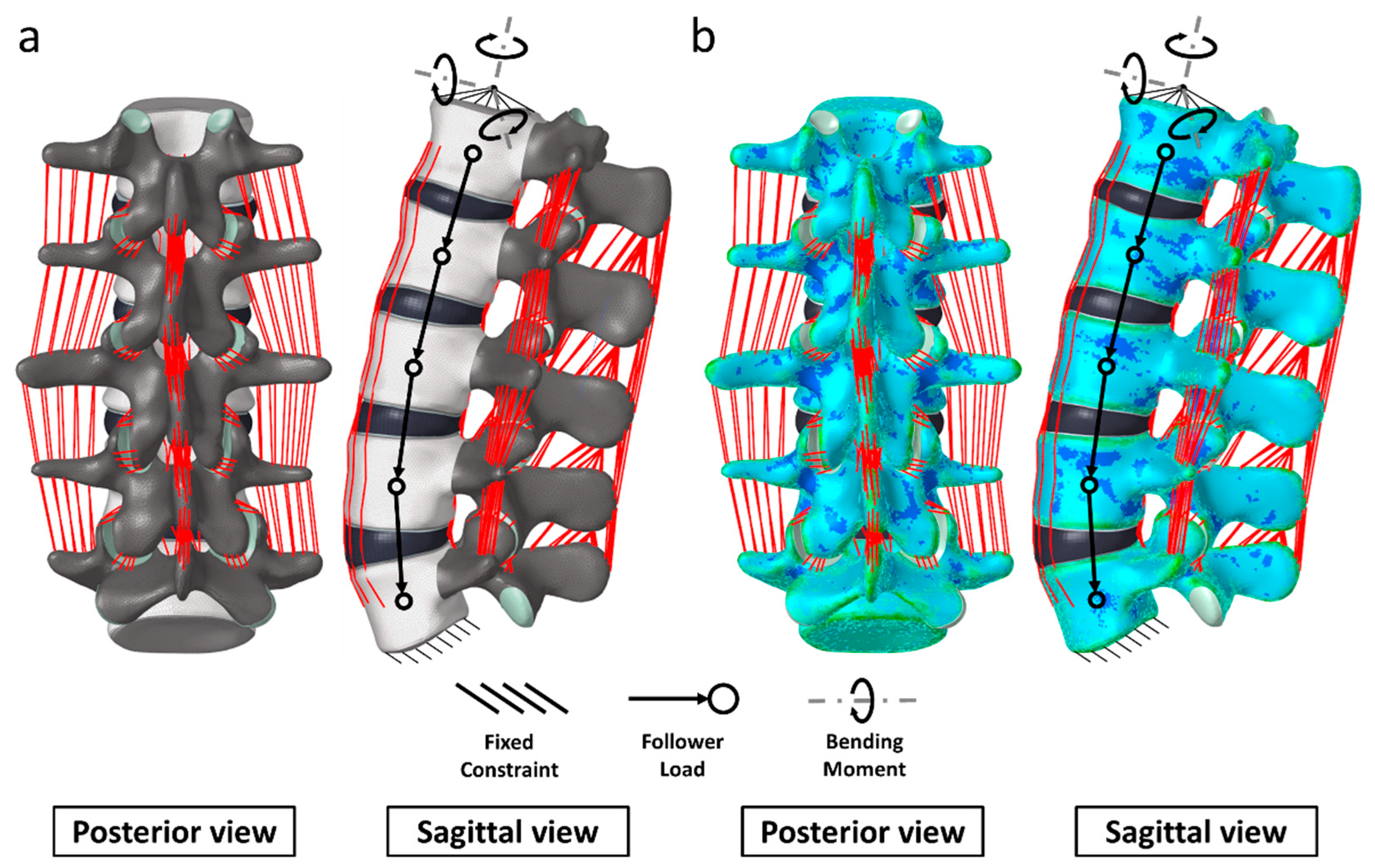
2.3. Loading and Boundary Conditions

To accurately validate the two finite element models, three different loading cases were applied in this study. First, a pure bending moment of 7.5 Nm was applied in the three anatomical planes at the cranial endplate of L1 to simulate flexion, extension, lateral bending, and axial rotation (Figure 2a,b) [48]. Second, to measure the IDP, a compressive follower load of 1000 N [49] was employed without any bending moments. The load was applied along a pre-optimised path through the centre of rotations of the vertebral bodies to minimise the presence of artefact bending moments (Figure 2a,b) [50]. The follower load technique considers both the effect of the upper body weight and the stabilising effect of the local muscle forces in compressive loading modes such as erect standing. Third, a combination of a compressive preload and a bending moment was used. The magnitude of the preload and moment for flexion, extension, lateral bending, and axial rotation were adopted from Dreischarf et al.: 1175 N with 7.5 Nm, 500 N with 7.5 Nm, 700 N with 7.8 Nm, and 720 N with 5.5 Nm, respectively [2]. During the simulations, the most caudal endplate of L5 was fixed in all degrees of freedom. The contact behaviour between the facet joint surfaces was assumed to be frictionless [51].

2.4. Mesh Convergence

To ensure that the mesh resolution did not affect the accuracy of model predictions, all elements of the bony parts of L4 vertebra was investigated with five different element lengths (0.607, 1, 1.65, 2.73, and 4.505 mm) for both modelling methods [11]. The edge length of the most refined mesh was determined based on the resolution of the CT. The mesh was considered convergent when the difference in the von Mises stress values was less than 10% compared to the most refined mesh [11,51]. As the results are most sensitive to axial rotation, a 7.5 Nm was applied on the upper vertebral endplate, while the lower endplate was fixed at all degrees of freedom [51,52].

2.5. Validation

The fully configured PSM and LBM with assigned material properties and applied loading and boundary conditions were exported from the pre-processor software HyperWorks to Abaqus Standard (v2021, Dassault Systemes, Vélizy-Villacoublay, France) to solve the finite element simulations.
Both the literature-based and patient-specific FE models were validated. Outcomes were compared with in vivo [53,54,55,56] and in vitro experimental measurements taken from the literature [57,58,59,60]. Dreischarf et al. have shown that comparison with diverse finite element results can increase the quality and reliability of the FE model’s prediction [2]. Therefore, the results of the current study were compared to multiple previously published well-accepted in silico data [2,29].
In the case of pure bending, the ROM, the intervertebral rotations (IVR), and the facet joint forces (FJF) were compared with in vitro [57,58,60] and in silico data [2,29] at each spinal level. In addition, the load-deflection curves of L1–L5 were plotted together with an in vitro measurement, and a range from numerical results. The ROM and IVR were calculated with an in-house developed MATLAB (MathWorks, Natick, Massachusetts, United States) script (Appendix B). Against pure compressive follower load, the intradiscal pressure (IDP) in the L4–L5 nucleus pulposus of both models was averaged over all elements and then compared with an in vitro [59] and a range of in silico results [2]. A combined compressive, and bending load was applied to the FE models to measure the IVR, FJF, and IDP values at each spinal level and compared with in silico [2] and in vivo measurements [53,54,55,56], as the combined loads are assumed to be the most representative for in vivo experiments [34].

2.6. Stress Distribution

In addition to the validation process, internal mechanical parameters were analysed to investigate the differences originating from the different modelling strategies applied. The Empirical Cumulative Distribution Functions (ECDF) of the von Mises stress values of all nodes in the vertebrae’s bony parts were plotted as a function of the load and material models applied (Figure S2). The ECDF is a step function that jumps up by 1/n at each n data point, where n is the number of von Mises stress values, practically equal to the number of nodes in the samples. At any specified von Mises stress value, ECDF gives the fraction of stress observations that are less or equal to that specified von Mises value [61]. Using MATLAB software, the ECDF estimated the cumulative distribution of the von Mises stress values in pure bending cases and both material models. The first and fifth lumbar vertebrae were excluded from this analysis to avoid data distortions due to load transfer and fixation.
ECDFs can describe the cumulative distribution of all nodes in the analysed sample but cannot characterise the maximum loaded state. To describe how the different bone material assignments affect the most compressed state of the vertebrae, 1% of the nodes with the smallest minimum principal (equivalent to highest compressive) strain from both models were analysed. Since PSM contained about tenfold more nodes than the LBM, a percentage-based selection was implemented instead of using an absolute number of nodes. In pure bending, all nodes of the bony regions were included in the sample, but L1 and L5 vertebrae were excluded to avoid compromised strain values due to load and boundary conditions applied to those regions. Boxplot figures with median strain values, whiskers, and outliers were plotted as a function of the loading cases for both LBM and PSM.

3. Results

3.1. Mesh Convergence

The mesh convergence test analysed the percentage differences in the von Mises stress of the L4 vertebra between the finest and coarser meshes. The differences in stress induced by the coarser meshes compared to the finest mesh were 28.76%, 14.96%, 10.02%, and 9.07%, in order of decreasing edge length for the LBM and 46.98%, 30.57%, 16.99%, and 2.73% for the PSM, respectively (Figure S3). For both the LBM and the PSM, the 1 mm mesh was the first to yield a difference of less than 10%, therefore found to converge for stress and was applied for both models.

3.2. Computational Times

The number of elements and the required computational time were compared. Due to the different FE meshing algorithms (LBM: adaptive meshing, PSM: uniform meshing), the PSM contained 12 million elements and the LBM 1.6 million elements. This difference resulted that, on average, the PSM took 12.1 times more to complete than the LBM against pure bending and compressive follower load. A similar trend was observed in the case of the combined load cases, namely that, on average, the PSM took 16.6 times more to finish the simulations (Figure S4).

3.3. Validation of the Lumbar Spine Models

3.3.1. Pure Bending Moment Load

For the total L1–L5 ROM in flexion-extension, lateral bending, and axial rotation, the results of the LBM and PSM were: 30.94°, 28.98°, 13.70°, and 31.58°, 28.55°, 14.12°, respectively. The predictions of the models were within the range of the experimental in vitro data [57] and the range of the in silico results of multiple FE simulations [2] (Figure 3a). Furthermore, the nonlinear load-deflection curves illustrate the stiffening behaviour of both FE models against larger loads (Figure 3b).
The mean FJF values were calculated as 51.15 N, 8.50 N, and 89.39 N for the LBM and 51.94 N, 8.50 N, and 83.74 N for the PSM, respectively, in extension, lateral bending, and axial rotation. Compared with the in vitro data [58], the predictions of the current study were slightly out of range in extension and close to the mid-value in axial rotation. The agreement with the in silico literature data was excellent for all load cases [2] (Figure 3c).
IVR values occurred within the range of experimental measurements [60], except at the L2–3 and L4–5 levels in flexion, where the models slightly underestimated the in vitro measurement, although our results correlate well with the in silico data [29]. In extension, the IVR values of the PSM were 4.57%, 6.14%, 8.65%, and 6.32% greater at the L1–2, L2–3, L3–4, and L4–5 spinal levels compared to the LBM (Figure 4a–d).

3.3.2. Pure Compression Load

The IDP values under the compressive follower load were 0.99 and 1.02 MPa for the LBM and PSM, respectively. The results were in good agreement with both the experimental results [59] and the in silico range [2] (Figure 3d).

3.3.3. Combined Load

Against combined load, the IVR results of the LBM and PSM were consistent with the available literature data, although the results in flexion at L2–3, L3–4 and L4–5 were outside the in vivo range [53,54,55]. The in silico range [2] was not reached in flexion at L1–2, in extension at L2–3 and L4–5, and in axial rotation at L1–2, L2–3 and L3–4. Compared to the LBM, the PSM provided greater IVR values in extension at all spinal levels (Figure 4e–g).
The IDP values showed good agreement with the published mean FE mid-values, while the simulation results approximated the available in vivo measurements [56] adequately. The PSM induced higher intradiscal pressure values in all loading conditions at all spinal levels (Figure 5).
The predicted facet joint forces were calculated at all spinal levels and compared to available in silico data [2]. The FJF values were not adaptable in flexion due to the lack of contact between the adjacent facet joint surfaces [2,51]. The outcomes of the current study were consistent with the existing literature data for all the applicable load cases. In agreement with other FE results, no contact occurred at L1–2, L2–3 and L3–4 in lateral bending [2]. The predicted FJF values were smaller at L1–2 and L2–3 in axial rotation than the FE ranges from the literature (Figure 6).

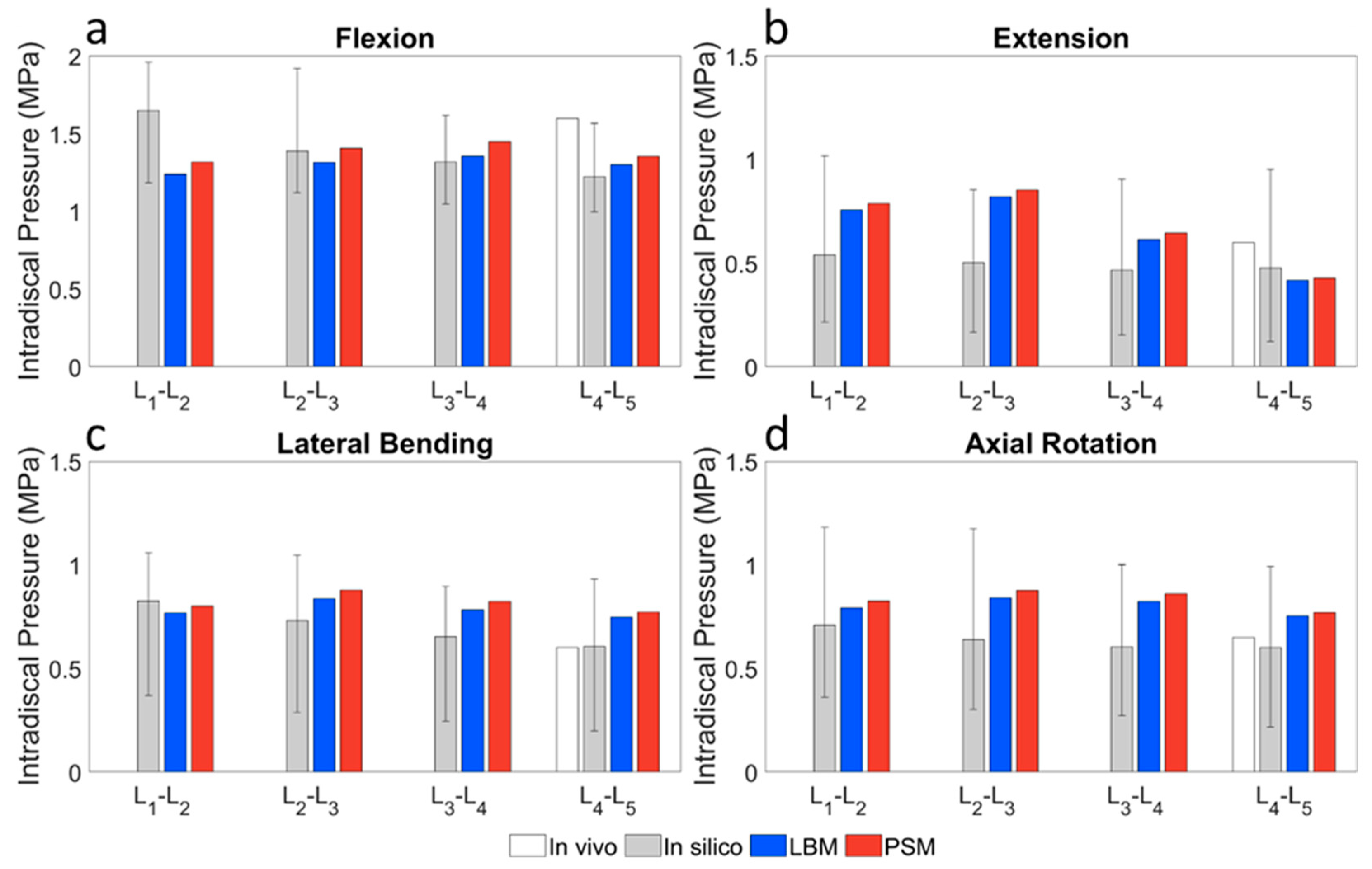
3.4. Stress Distributions

The ECDF plots of the estimated cumulative distribution showed noteworthy differences between the models developed by two bone material assignment strategies (Figure 7a–d). Generally, the cumulative distribution of stress values in the low-stress range, from 0 MPa to 1 MPa, shows the same characteristics. It is also observed that the stress values in the LBM are more spread out and have a less steep curve than in the PSM. This difference in the curve steepness also means that proportionally, the LBM contains more high-stress elements.
The strain values characterise the most compressed state of the bony tissues, as nodes with the smallest minimum principal (equivalent to highest compressive) strain were included in this analysis. In the LBM, the median compressive strain values were calculated as −0.0053, −0.0040, −0.0059, and −0.0023 for flexion, extension, lateral bending, and axial rotation, respectively. In contrast to the LBM, the PSM decreased median compressive strain values by 77.3%, 62.5%, 79.7%, and 39.1%, respectively (Figure 8). Although the outlier values reveals that the PSM spreads the strain values more evenly, as the box and whiskers are narrow, and contains more outliers than the LBM. While the median values are lower in the LBM, the outliers are even lower in the PSM, indicating that the PSM includes more nodes with higher compression.

4. Discussion

The current study presents and compares two different bone material assignment strategies commonly used in FE-based biomechanical investigations. Verification of the developed FE meshes was performed through a mesh convergence study to ensure proper simulation predictions. Then, the developed models were validated using numerous biomechanical parameters, such as ROM, IVR, IDP, and FJF. Furthermore, the required computational time, cumulative distribution of the stress values and the compressive strain values in the bony elements of the L2, L3, and L4 vertebra were assessed. The specificities, challenges, and limitations of these techniques were highlighted.

4.1. Locally Defined Material Properties

Clinical application of bone imaging for the in vivo assessment of structural properties involves, among others, dual X-ray absorptiometry (DXA), quantitative computed tomography (QCT), quantitative ultrasonometry (QUS), and high-resolution magnetic resonance (HR-MR) [62]. These non-invasive and non-destructive techniques are coupled with different advantages and disadvantages. DXA and QCT need ionising radiation, while HR-MR and QUS apply no radiation load on the patient [63]. Using the QUS technique in vivo, the number of measurement sites is limited; there is also little opportunity for calibration standardisation [63,64]. In contrast to QUS, the QCT technique can provide accurate data on the 3D BMD of the trabecular and cortical compartments via calibration. HR-MR acquisition takes much more time and is technically demanding, although, in contrast to DXA, the apparent microstructure of the bone is assessable, likewise with QCT [62,65].
In addition to these techniques, finite element models employing locally defined material properties have been used to evaluate fracture risk and ultimate strength and have shown superior results in comparison with densitometry measurements alone [62,65]. Due to the relative availability of QCT scans and the possibility of accurately modelling locally defined material properties in FE models, the current study employed QCT-derived materials in the patient-specific model.
Multiple studies have defined empirical relationships for assigning local material properties based on QCT for different anatomic sites by comparing the QCT-based bone density with the results of mechanical testing [40,66,67,68]. According to Carpenter et al. [69], the QCT-based bone density can be directly converted into local mechanical properties when using calibration phantoms, which approach has been used in several finite element studies in various anatomical areas [19,37,70,71,72]. The finite element models typically used voxel-based hexahedral elements [37,72,73,74] or tetrahedral elements that follow the smoothed geometry [19,36,70,71,75]. Density assignment is more directly implemented in voxel-based models, where voxels are directly converted into hexahedral elements, and thus the density of an element is equal to the density of the corresponding voxel of the QCT scan [37]. On the contrary, tetrahedral-based models better approximate the complex structure and geometry of vertebrae than hexahedral ones [76]. However, as Imai et al. [77] stated, in these models, the density of an element is the average density of the voxels contained in one element, which clearly shows why QCT resolution and mesh resolution is important [11]. Furthermore, Morgan et al. [40] concluded that modulus-density relationships depend on the anatomic site, which means there is no universal modulus–density relationship, so it is essential that the used relationship comes from the same anatomical site as the one being investigated. Accordingly, in our research, besides applying a thin-sliced QCT imaging protocol [22] and accurate tetrahedral mesh resolution [11], we implemented a commonly used, well-established correlation that has been determined based on in vitro measurements of vertebrae [40].

4.2. Mesh Convergence

Although in the literature, the displacement [78] and strain energy [52,76] are also used as parameters of mesh convergence, the von Mises stress was chosen since mesh resolution is more sensitive to internal mechanical parameters than displacement [52]. Based on the results, the PSM is more sensitive to the mesh resolution in terms of stress due to its element-based material assignment strategy (Figure S3). In contrast, in the LBM, relatively minor stress changes occurred due to the homogeneous modelling of different anatomical sections. Both the LBM and PSM gave results less than 10% at 1 mm element size, agreeing with the findings of Costa et al. [11], who applied an identical imaging protocol and similar bone material assignment strategy. The required computational time of the models with the finest mesh increased significantly compared to the 1 mm results, which also reinforced the choice of the 1 mm element since the elevated computational demand does not couple with higher accuracy (Figure S3).

4.3. Computational Times

In general, applying the literature-based modelling approach reduced the required CPU time since the PSM notably needed more time to complete for both the pure and combined loads. In the case of the patient-specific bone material assignment, the computational cost dramatically increased due to the different meshing algorithms applied for the two models. However, it is worth mentioning that the patient-specific model required less time to develop than the literature-based model considering the soft tissues are the same for both models. Since segmentation is required for both models, the difference is due to the design of the bony parts, as the calibration between Hounsfield Units and densities is based on segmented calibration phantoms that take less time than the separation of the cortical part, the trabecular part, the posterior elements, and the bony endplates for each vertebra.

4.4. Model Validation

Results of the current study were compared with available in vitro and in silico data from the literature. Dreischarf et al. described that the validation via diverse results increase the accuracy and reliability of the developed models’ predictions [2]. Therefore, validation was performed in the current study utilising several published experimental and in silico results. The LBM and PSM yielded similar ROM results against pure bending moment of 7.5 Nm indicating that the material assignment of the bony structures slightly influences the spinal kinematics of the spine. Similar findings were described by Vena et al., stating that for FE simulations, the material properties of the bony structures have a minor influence on the spinal kinematics; thus, vertebral bodies could be modelled as rigid bodies [79]. Moreover, Remus et al. presented, calibrated, and validated a hybrid finite element-multibody model with rigid vertebral bodies, indicating that the hybrid simulation model is powerful and efficient for providing valid mechanical responses. Their study confirmed that the soft tissues such as the spinal ligaments and the IVD have primarily influence the kinematic properties of the spine [29]. Thus, nonlinear modelling of such structures is crucial, and therefore in the current study, the spinal ligaments and components of the intervertebral discs were modelled with nonlinear materials. The two models were in a good agreement with the published in silico and in vitro studies in L1–L5 ROM of flexion-extension, lateral bending, and axial rotation. However, the nonlinear load-displacement curve (Figure 3b) demonstrates that in flexion, both the patient-specific and literature-based models are slightly outside the in vitro range, while in extension, the LBM is within, the PSM is slightly outside the range. The same trend is reported by Dreischarf et al. [2], that majority of their assessed FE models overestimate the motion in extension and underestimate it in flexion, moreover, good agreement was found with the reported in silico results for lateral bending and axial rotation as well [2].
The FJF depends on several patient-specific factors, such as the underlying geometry of the individual cartilage surfaces, the gap size between the adjacent surfaces, or the thickness of the cartilage layer [80]. There is limited data available in the literature on the in vitro measurement of FJF, and these studies have some limitations and uncertainties [51]. Nevertheless, in pure bending, the results of the current study show good agreement with the available in vitro [58] and in silico [2] data, although a slight overestimation of the in vitro result appeared in extension (Figure 3c). The current study results indicate that the FJF in lateral bending is notably lower than in extension and axial rotation, which may originate from the patient-specific anatomy of the current study’s FE model agreeing with the findings of Woldtvedt et al. [80]. In flexion, no force was transmitted due to the distancing cartilage surfaces during the load [34].
The IDP predictions of the FE models in pure compressive follower load showed excellent agreement with the median in vitro results at 300 N and 1000 N (Figure 3d). Among the published FE models in the literature, the NP is often modelled as incompressible fluid-filled cavity [25,49], which allows simulating the effect of the initial hydrostatic pressure in the IVD [81]. Nonetheless, as Dreischarf et al. pointed out, most NPs modelled with fluid-filled cavities neglect this effect since IDP values measured in the unloaded state are less significant [2].
The IVR values were obtained and evaluated for both pure and combined load cases (Figure 4a–h). Wilke et al. previously reported that 7.5 Nm pure bending moment is the most appropriate for simulating the loads on the lumbar section, including effects of muscle forces [48]. Panjabi et al. performed a human cadaveric test [60], while Remus et al. presented a hybrid FE-multibody analysis to investigate the biomechanical properties of the human lumbar spine [29]. Accordingly, the IVR results of these in vitro and in silico studies have been used as a basis for comparison in the case of pure bending load. The employed combined loads were determined by Rohlmann et al. and Dreischarf et al., using follower load and bending moment combination that most closely approximates the average of in vivo measurements reported in the literature [34,82,83]. In the case of the combined load, the average of three in vivo measurements [53,54,55] was used as a basis for comparison when evaluating the IVR results. In both load cases, the FE predictions of the current study agree with the experimental results in extension, lateral bending, and axial rotation, while the simulations underestimated the experimental results in flexion. The predictions of the current study are comparable to the in silico findings reported by Remus et al. and Dreischarf et al. [2,29].
The predicted IDP values for combined load were compared to the mean of eight well-accepted in silico results [2]. Moreover, Wilke et al. performed an in vivo analysis in a non-degenerative L4–L5 IVD [56]. Their study was designed to provide a validation dataset for in silico or in vitro investigations. Excellent agreement with the in vivo and in silico results indicates that both models can predict the intradiscal pressure values accurately.
In the case of combined load, the FJF values were compared only to those mean in silico results reported by Dreischarf et al. due to the lack of relevant experimental results [2]. In general, the validated in silico studies show a significant variance regarding the FJF’s magnitude, indicating that this force is sensitive to the FE modelling techniques and the patient-specific anatomy. This finding is also supported by Schmidt et al., who found that the FJF is highly dependent on the individual geometry of facet joint surfaces [84]. In flexion, no force occurred due to the lack of contact. In extension, the magnitude of the FJF increases caudally, agreeing to the results reported by Remus et al. [29]. In lateral bending, FJF occurred only at the L4–L5 spinal level, as it was reported in several models investigated by Dreischarf et al. [2].

4.5. Stress Distributions

The plot of the cumulative distribution of stress values highlights the fundamental difference between the LBM and PSM. The differences in the high-stress (above 1 MPa) range’s distribution indicate that the application of patient-specific bone materials yields substantially different internal mechanical properties. The difference in the slope between the distribution curves is the largest for axial rotation, which agrees with the findings of Ayturk. et al. [52], i.e., the stress distribution of finite element models is most sensitive to axial rotation. The analysis of the minimum principal strain values also concludes that the two models show significant differences in internal mechanical parameters under the same loading conditions. In the LBM model, the strain values cluster around a peak with only a few outliers, while in the PSM, no such strain peak is observed. The clustering effect explains why the LBM gave lower median values than the PSM; since investigating the outliers, one can see that the PSM contains bony tissues with higher compression. Based on these findings, using medical imaging-based bone material properties could be beneficial in biomechanical investigations where it is essential to analyze internal mechanical parameters, i.e., vertebral fracture risk or vertebral strength assessment [11,17,18]. These conclusions confirm the findings of Mosleh et al., who found a good correlation between the fracture loads estimated by QCT-based FE models and in-vitro fracture loads [85]. Moreover, a biomechanical study by Rezaei has shown how QCT combined FE simulations can estimate fracture outcomes in single vertebral models [86]. Analogously, literature-based linearly elastic homogeneous material models can only be used carefully in cases where bone material quality significantly influences the parameters to be investigated.

4.6. Limitations, Significance

Like most finite element analyses, the current study also has limitations and simplifications worth highlighting. By its very nature, the FE method cannot address biological or physiological phenomena, as it solely works on a mechanical principle. The viscoelastic and poroelastic characteristic of the IVD was not considered since a quasi-static analysis was performed, and different time-dependent behaviours, such as creep, were not the interest of the current study. Additionally, the presented models have the potential for further development, with considering the effect of muscle forces, increasing the number of material groups in patient-specific bone material assignment, or modelling the NP as an incompressible fluid cavity and include initial hydrostatic pressure field. Although the models could be improved by addressing these simplifications, we believe that the relationship between the models and their results would not change; thus, the presented and validated models are suitable for drawing conclusions and for further biomechanical investigations.

5. Conclusions

The current study aimed to present two commonly used bone material assigning techniques to develop a finite element model of the healthy human lumbar spine. Mesh resolution was investigated to ensure accurate model predictions. The results of the FE models were compared with in vivo, in vitro, and well-accepted in silico data from the literature to validate them. Validation was performed considering ROM, IVR, IDP, and FJF variables against pure, and combined loads. Based on the parameters and loads investigated, both the LBM and PSM can be used to model the biomechanical properties, such as ROM, IVR, FJF, and IDP of the lumbar spine, as they are in good agreement with the previously published results in most investigated variables. However, substantial differences in computational time and cumulative distribution of von Mises stress values were observed between the literature-based and the patient-specific models.

Supplementary Materials

The following supporting information can be downloaded at: https://www.mdpi.com/article/10.3390/app122010256/s1, Figure S1: The nonlinear stress-strain relationships of the six different annulus fibre layers in the intervertebral disc. Layer 1 is the outermost and layer 6 is the innermost layer; Figure S2: Schematic representation of the building steps to plot the empirical cumulative distribution functions; Figure S3. Von Mises stress and computational time of meshes with different edge lengths in the case of literature-based model (a) and patient-specific model (b); Figure S4: Required computational times for the LBM and PSM against (a) pure and (b) combined loads; Code S1: Calculation of the investigated variables.

Author Contributions

Conceptualization, P.E.E., A.L., G.S. and Z.H.; Methodology, P.E.E.; Software, A.J.P.; Validation, M.T.; Investigation, M.T. and A.J.P.; Data Curation: M.T., A.J.P., R.M.K. and P.E.E.; Writing—Original Draft Preparation, M.T., A.J.P. and P.E.E.; Writing—Review & Editing, A.L.; Visualization, M.T. and A.J.P.; Supervision, P.E.E. and A.L. All authors have read and agreed to the published version of the manuscript.

Funding

This work was supported by the Hungarian Scientific Research Fund grant Budapest, Hungary, (OTKA FK123884), and by the New National Excellence Program (ÚNKP-21-5) and the Doctoral Student Scholarship Program (C1014064) of the Co-Operative Doctoral Program of the Ministry of Innovation and Technology, Hungary, financed from the National Research, Development and Innovation Fund. The financial support from these funding bodies is gratefully acknowledged.

Institutional Review Board Statement

Ethical Approval was given by the National Ethics Committee of Hungary and the National Institute of Pharmacy and Nutrition (reference number: OGYÉI/163-4/2019).

Informed Consent Statement

Informed consent was obtained from all subjects involved in the study.

Data Availability Statement

The extracted data and the applied code of this investigation are appended as Supplementary Material to this article. In addition to the code, its detailed description, figures and file structure are shared for the sake of clarity and reproducibility. The authors believe that the “Materials and Methods” section, the appendices, and the developed in-house code cover the investigated topics satisfactorily.

Acknowledgments

The support of CAD-Terv Kft. in using Abaqus, especially of István Nadj and Gábor Brezvai, is highly acknowledged.

Conflicts of Interest

The authors declare no conflict of interest.

Appendix A

The attachment points and orientation of the elements modelling the ligaments were adopted from a previously published study, MySPINE [22]. All seven major spinal ligaments were modelled: anterior longitudinal ligament (ALL), posterior longitudinal ligament (PLL), ligamentum flavum (LF), interspinous ligament (ISL), supraspinous ligament (SSL), intertransverse ligament (ITL), and capsular ligaments (CL). In the current study the ligaments were modelled with multiple spring elements in either parallel-series connection (ALL, PLL) or in parallel connection only (ISL, CL, ITL, LF, PLL, SSL) (Table A1) [44].
Table A1. Nonlinear force-stiffness characteristics of the ligaments.
LigamentNo. ElementsLength of 1 Element (mm), LeLength of 1 Chain (mm), Lchain
ALL5 parallel, 4 in series10.3641.44
ISL24 in parallel6.866.86
CL20 in parallel6.546.54
ITL20 in parallel22.5022.50
LF7 in parallel14.0814.08
PLL5 parallel, 4 in series8.5634.24
SSL6 in parallel15.1415.14
Rohlmann et al. defined the nonlinear characteristic for each ligament with two variables, stiffness, and strain. Data from Rohlmann et al. can be rewritten in the following form and units [47] (Table A2).
Table A2. Number, connection type, and length of elements in the ligaments [47].
LigamentK1
(N/mm)
ε1
(-)
K2
(N/mm)
ε2
(-)
K3
(N/mm)
ALL3470.1227870.2031864
ISL1.40.1391.50.20014.7
CL360.2501590.300384
ITL0.30.1821.80.23310.7
LF7.70.0599.60.49058.2
PLL29.50.11161.70.230236
SSL2.50.2005.30.25034
As presented, Rohlmann et al. [47] defined the spring-like behaviour of the ligaments with strain dependent stiffness value of a single spring, describing the progressive characteristic. Nonlinear spring characteristic should be defined in Abaqus with force and elongation value pairs assigned to the corresponding SPRINGA element sets. To assign the material properties correctly, the following calculations were applied:
F ε = K 1 L 0 ε , i f     0 < ε ε 1 K 1 L 0 ε 1 + K 2 L 0 ε ε 1 ,   i f     ε 1 < ε ε 2 K 1 L 0 ε 1 + K 2 L 0 ε 2 + K 3 L 0 ε ε 2 , i f     ε 2 < ε 1
For the sake of simplicity, 1 was chosen as an upper limit of the ligament strains, since 100% strain is not reached during the simulation, thus the calculation remains stable. From this, the elementary force can be calculated (the force which is assigned to each element):
F e = 1 p F ε
Beside the force values Abaqus requires the corresponding elongation values (strain dependent and elementary) as well:
D ε = L c h a i n ε
D e = 1 s D ε = 1 s L c h a i n ε ,
where:
  • F —force (N)
  • p —number of parallel chains (-)
  • s —number of elements in a chain (-)
  • K n —stiffness (N/mm)
  • ε n —strain (-)
  • D —elongation (mm)
  • L 0 —average length of one element (mm)
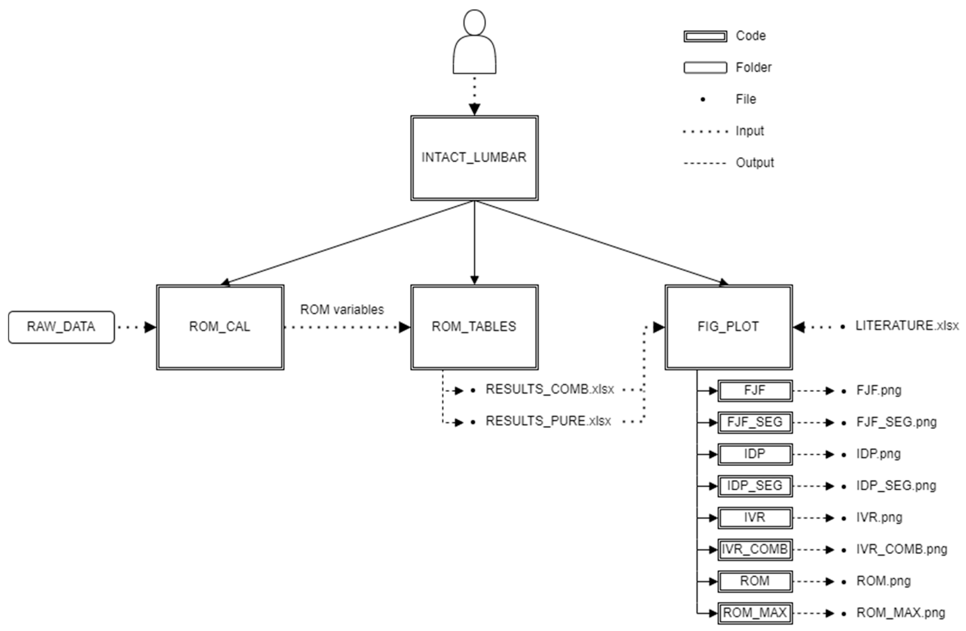
The applied material properties defined by Rohlmann [47] were plotted in Figure A1, where the progressive behaviour of the ligaments is visualised.
Figure A1. The nonlinear force-strain relationships of the seven spinal ligaments applied in the current study.
Applsci 12 10256 g0a1

Appendix B

Calculation of the investigated variables from the finite element analysis is challenging. The current study considered two force, two pressure, and four rotation variables. The force (FJF, FJF_SEG) and pressure (IDP, IDP_SEG) variables can be calculated using average and maximum calculations after summary of the exported data. The calculation of the rotation variables (IVR, IVR_COMB, ROM, ROM_MAX) was based on virtual markers. The markers were nodes coupled to the vertebrae with rigid coupling. Three markers were used for each vertebra: middle points of the upper and lower endplate and a point in the middle sagittal plane of the spinous process (Figure A2).
Figure A2. Markers on a vertebra (a) Posterior isometric view from below (b) Posterior isometric view from above (c) Front view (d) Transparent anterior isometric view, UP: Upper Point, LP: Lower Point, PP: Posterior Point.
Applsci 12 10256 g0a2
For each vertebra, the middle points of the endplates define an axis and the three markers define a plane, so a local coordinate system can be created according to Panjabi and White [30] (Figure A3). The definition of the axes means the sign of the rotations is as follows: positive: flexion, left rotation, right bending; negative: extension, right rotation, left bending.
Figure A3. Local coordinate system of a vertebra.
Applsci 12 10256 g0a3
The rotation variables were calculated based on these local coordinate systems (LCSs) of the vertebrae: the rotation of a segment (IVR, IVR_COMB) was calculated as the rotation of the upper vertebra’s LCS expressed in the lower vertebra’s LCS. The rotation of the whole lumbar spine (ROM, ROM_MAX) was calculated likewise: the rotation of the top vertebra’s LCS expressed in the bottom vertebra’s LCS. To calculate these rotations, the calculation of a rotation matrix for each LCS is necessary since the coordinates of the markers are given in the global coordinate system.
Code S1 contains a folder structure (Figure A4) and a MATLAB code structure (Figure A5) which help with the calculation and visualisation of the above-mentioned variables. The user should load data to the right places in the RAW_DATA folder based on its type and run INTACT_LUMBAR.m in the MATLAB folder. When the code finished, the figures can be found in the PICTURES folder.
Figure A4. Folder Structure.
Applsci 12 10256 g0a4
The purpose and content of the folders:
  • DIAG_TABLES: contains 3 tables: LITERATURE, RESULTS_PURE and RESULTS_COMB which contain data necessary for the plotting of the diagrams.
  • MATLAB: contains the main code INTACT_LUMBAR and folders below:
    ROM: contains the calculating and exporting codes, which use tables from RAW_DATA folder as input and write sheets in tables in DIAG_TABLES folder as output
    PLOT: contains the plotting codes
  • PICTURES: contains the figures of the investigated variables
  • RAW_DATA: contains tables of the raw data of the investigated variables
    COMBINED_LOADS: contains tables in the case of combined loads
    LBM: contains data of the literature-based model
    • IDP_DATA: contains rpt files exported from Abaqus for IDP calculation
    PSM: contains data of the patient-specific model
    • IDP_DATA: contains rpt files exported from Abaqus for IDP calculation
    PURE_LOADS: tables in the case of pure loads
    LBM: contains data of the literature-based model
    • IDP_DATA: contains rpt files exported from Abaqus for IDP calculation
    PSM: contains data of the patient-specific model
    • IDP_DATA: contains rpt files exported from Abaqus for IDP calculation
The code consists of four MATLAB files:
  • INTACT_LUMBAR: main code, handle data input and runs the three other main functions,
  • ROM_CAL: function for rotation calculation. Input: tables from RAW_DATA, Output: internal ROM variables,
  • ROM_TABLES: function for data arrangement and export. Input: internal ROM variables, Output: result tables,
  • FIG_PLOT: function for visualisation of the results. Input: result tables and a table containing literature results, Output: figures of the investigated variables.
Figure A5. Code Structure.
Applsci 12 10256 g0a5

References

  1. Schmidt, H.; Galbusera, F.; Rohlmann, A.; Shirazi-Adl, A. What Have We Learned from Finite Element Model Studies of Lumbar Intervertebral Discs in the Past Four Decades? J. Biomech. 2013, 46, 2342–2355. [Google Scholar] [CrossRef]
  2. Dreischarf, M.; Zander, T.; Shirazi-adl, A.; Puttlitz, C.M.; Adam, C.J.; Chen, C.S.; Goel, V.K.; Kiapour, A.; Kim, Y.H.; Labus, K.M.; et al. Comparison of Eight Published Static Finite Element Models of the Intact Lumbar Spine: Predictive Power of Models Improves When Combined Together. J. Biomech. 2014, 47, 1757–1766. [Google Scholar] [CrossRef] [Green Version]
  3. Fagan, M.J.; Julian, S.; Mohsen, A.M. Finite Element Analysis in Spine Research. Proc. Inst. Mech. Eng. Part H J. Eng. Med. 2002, 216, 281–298. [Google Scholar] [CrossRef]
  4. Little, J.P.; Adam, C.J. Geometric Sensitivity of Patient-Specific Finite Element Models of the Spine to Variability in User-Selected Anatomical Landmarks. Comput. Methods Biomech. Biomed. Eng. 2013, 18, 676–688. [Google Scholar] [CrossRef]
  5. Viceconti, M.; Pappalardo, F.; Rodriguez, B.; Horner, M.; Bischoff, J.; Tshinanu, F.M. In Silico Trials: Verification, Validation and Uncertainty Quantification of Predictive Models Used in the Regulatory Evaluation of Biomedical Products. Methods 2021, 185, 120–127. [Google Scholar] [CrossRef]
  6. Viceconti, M.; Henney, A.; Morley-Fletcher, E. In Silico Clinical Trials: How Computer Simulation Will Transform the Biomedical Industry. Int. J. Clin. Trials 2016, 3, 37. [Google Scholar] [CrossRef] [Green Version]
  7. Pappalardo, F.; Russo, G.; Tshinanu, F.M.; Viceconti, M. In Silico Clinical Trials: Concepts and Early Adoptions. Brief. Bioinform. 2019, 20, 1699–1708. [Google Scholar] [CrossRef]
  8. La Barbera, L.; Larson, A.N.; Rawlinson, J.; Aubin, C.-E. In Silico Patient-Specific Optimization of Correction Strategies for Thoracic Adolescent Idiopathic Scoliosis. Clin. Biomech. 2021, 81, 105200. [Google Scholar] [CrossRef]
  9. Agarwal, A.; Agarwal, A.K.; Jayaswal, A.; Goel, V.K. Outcomes of Optimal Distraction Forces and Frequencies in Growth Rod Surgery for Different Types of Scoliotic Curves: An in Silico and in Vitro Study. Spine Deform. 2017, 5, 18–26. [Google Scholar] [CrossRef]
  10. Vergari, C.; Gaume, M.; Persohn, S.; Miladi, L.; Skalli, W. From in Vitro Evaluation of a Finite Element Model of the Spine to in Silico Comparison of Spine Instrumentations. J. Mech. Behav. Biomed. Mater. 2021, 123, 104797. [Google Scholar] [CrossRef]
  11. Costa, M.C.; Eltes, P.; Lazary, A.; Varga, P.P.; Viceconti, M.; Dall’Ara, E. Biomechanical Assessment of Vertebrae with Lytic Metastases with Subject-Specific Finite Element Models. J. Mech. Behav. Biomed. Mater. 2019, 98, 268–290. [Google Scholar] [CrossRef]
  12. Xiao, Z.; Wang, L.; Gong, H.; Zhu, D.; Zhang, X. A Non-Linear Finite Element Model of Human L4-L5 Lumbar Spinal Segment with Three-Dimensional Solid Element Ligaments. Theor. Appl. Mech. Lett. 2011, 1, 064001. [Google Scholar] [CrossRef] [Green Version]
  13. Shirazi-Adl, A. Biomechanics of the Lumbar Spine in Sagittal/Lateral Moments. Spine 1994, 19, 2407–2414. [Google Scholar] [CrossRef]
  14. Park, W.M.; Kim, K.; Kim, Y.H. Effects of Degenerated Intervertebral Discs on Intersegmental Rotations, Intradiscal Pressures, and Facet Joint Forces of the Whole Lumbar Spine. Comput. Biol. Med. 2013, 43, 1234–1240. [Google Scholar] [CrossRef]
  15. Schmidt, H.; Galbusera, F.; Rohlmann, A.; Zander, T.; Wilke, H.J. Effect of Multilevel Lumbar Disc Arthroplasty on Spine Kinematics and Facet Joint Loads in Flexion and Extension: A Finite Element Analysis. Eur. Spine J. 2012, 21, 663–674. [Google Scholar] [CrossRef] [Green Version]
  16. Li, J.; Shang, J.; Zhou, Y.; Li, C.; Liu, H. Finite Element Analysis of a New Pedicle Screw-Plate System for Minimally Invasive Transforaminal Lumbar Interbody Fusion. PLoS ONE 2015, 10, e0144637. [Google Scholar] [CrossRef] [Green Version]
  17. Faulkner, K.G.; Cann, C.E.; Hasegawa, B.H. Effect of Bone Distribution on Vertebral Strength: Assessment with Patient-Specific Nonlinear Finite Element Analysis. Radiology 1991, 179, 669–674. [Google Scholar] [CrossRef]
  18. Crawford, R.P.; Cann, C.E.; Keaveny, T.M. Finite Element Models Predict in Vitro Vertebral Body Compressive Strength Better than Quantitative Computed Tomography. Bone 2003, 33, 744–750. [Google Scholar] [CrossRef]
  19. Groenen, K.H.J.; Bitter, T.; van Veluwen, T.C.G.; van der Linden, Y.M.; Verdonschot, N.; Tanck, E.; Janssen, D. Case-Specific Non-Linear Finite Element Models to Predict Failure Behavior in Two Functional Spinal Units. J. Orthop. Res. 2018, 36, 3208–3218. [Google Scholar] [CrossRef] [Green Version]
  20. O’Reilly, M.A.; Whyne, C.M. Comparison of Computed Tomography Based Parametric and Patient-Specific Finite Element Models of the Healthy and Metastatic Spine Using a Mesh-Morphing Algorithm. Spine 2008, 33, 1876–1881. [Google Scholar] [CrossRef]
  21. Sapin-De Brosses, E.; Jolivet, E.; Travert, C.; Mitton, D.; Skalli, W. Prediction of the Vertebral Strength Using a Finite Element Model Derived from Low-Dose Biplanar Imaging: Benefits of Subject-Specific Material Properties. Spine 2012, 37, E156–E162. [Google Scholar] [CrossRef] [PubMed]
  22. Van Rijsbergen, M.; Van Rietbergen, B.; Barthelemy, V.; Eltes, P.; Lazáry, Á.; Lacroix, D.; Noailly, J.; Tho, M.C.H.B.; Wilson, W.; Ito, K. Comparison of Patient-Specific Computational Models vs. Clinical Follow-up, for Adjacent Segment Disc Degeneration and Bone Remodelling after Spinal Fusion. PLoS ONE 2018, 13, e0200899. [Google Scholar] [CrossRef] [Green Version]
  23. Aryanto, K.Y.E.; Oudkerk, M.; van Ooijen, P.M.A. Free DICOM De-Identification Tools in Clinical Research: Functioning and Safety of Patient Privacy. Eur. Radiol. 2015, 25, 3685–3695. [Google Scholar] [CrossRef] [PubMed] [Green Version]
  24. Bereczki, F.; Turbucz, M.; Kiss, R.; Eltes, P.E.; Lazary, A. Stability Evaluation of Different Oblique Lumbar Interbody Fusion Constructs in Normal and Osteoporotic Condition—A Finite Element Based Study. Front. Bioeng. Biotechnol. 2021, 9, 749914. [Google Scholar] [CrossRef] [PubMed]
  25. Shirazi-Adl, S.A.; Shrivastava, S.C.; Ahmed, A.M. Stress Analysis of the Lumbar Disc-Body Unit in Compression. A Three-Dimensional Nonlinear Finite Element Study. Spine 1984, 9, 120–134. [Google Scholar] [CrossRef]
  26. Baroud, G.; Nemes, J.; Heini, P.; Steffen, T. Load Shift of the Intervertebral Disc after a Vertebroplasty: A Finite-Element Study. Eur. Spine J. 2003, 12, 421–426. [Google Scholar] [CrossRef] [Green Version]
  27. Finley, S.M.; Brodke, D.S.; Spina, N.T.; DeDen, C.A.; Ellis, B.J.; Finley, S.M.; Brodke, D.S.; Spina, N.T.; DeDen, C.A. FEBio Finite Element Models of the Human Lumbar Spine. Comput. Methods Biomech. Biomed. Eng. 2018, 21, 444–452. [Google Scholar] [CrossRef]
  28. Zeng, Z.L.; Zhu, R.; Wu, Y.C.; Zuo, W.; Yu, Y.; Wang, J.J.; Cheng, L.M. Effect of Graded Facetectomy on Lumbar Biomechanics. J. Healthc. Eng. 2017, 2017, 7981513. [Google Scholar] [CrossRef] [Green Version]
  29. Remus, R.; Lipphaus, A.; Neumann, M.; Bender, B. Calibration and Validation of a Novel Hybrid Model of the Lumbosacral Spine in ArtiSynth–The Passive Structures. PLoS ONE 2021, 16, e0250456. [Google Scholar] [CrossRef]
  30. Panjabi, M.M.; White, A.A. Clinical Biomechanics of the Spine; Lippincott: Philadelphia, PA, USA, 1990; ISBN 9780323026222. [Google Scholar]
  31. Noailly, J.; Wilke, H.J.; Planell, J.A.; Lacroix, D. How Does the Geometry Affect the Internal Biomechanics of a Lumbar Spine Bi-Segment Finite Element Model? Consequences on the Validation Process. J. Biomech. 2007, 40, 2414–2425. [Google Scholar] [CrossRef]
  32. Rohlmann, A.; Burra, N.K.; Zander, T.; Bergmann, G. Comparison of the Effects of Bilateral Posterior Dynamic and Rigid Fixation Devices on the Loads in the Lumbar Spine: A Finite Element Analysis. Eur. Spine J. 2007, 16, 1223–1231. [Google Scholar] [CrossRef] [PubMed] [Green Version]
  33. Lu, Y.M.; Hutton, W.C.; Gharpuray, V.M. Do Bending, Twisting, and Diurnal Fluid Changes in the Disc Affect the Propensity to Prolapse? A Viscoelastic Finite Element Model. Spine 1996, 21, 2570–2579. [Google Scholar] [CrossRef] [PubMed]
  34. Rohlmann, A.; Zander, T.; Rao, M.; Bergmann, G. Realistic Loading Conditions for Upper Body Bending. J. Biomech. 2009, 42, 884–890. [Google Scholar] [CrossRef] [PubMed]
  35. Shirazi-Adl, A.; Ahmed, A.M.; Shrivastava, S.C. Mechanical Response of a Lumbar Motion Segment in Axial Torque Alone and Combined with Compression. Spine 1986, 11, 914–927. [Google Scholar] [CrossRef] [PubMed]
  36. Tawara, D.; Sakamoto, J.; Murakami, H.; Kawahara, N.; Oda, J.; Tomita, K. Mechanical Evaluation by Patient-Specific Finite Element Analyses Demonstrates Therapeutic Effects for Osteoporotic Vertebrae. J. Mech. Behav. Biomed. Mater. 2010, 3, 31–40. [Google Scholar] [CrossRef]
  37. Nishiyama, K.K.; Gilchrist, S.; Guy, P.; Cripton, P.; Boyd, S.K. Proximal Femur Bone Strength Estimated by a Computationally Fast Finite Element Analysis in a Sideways Fall Configuration. J. Biomech. 2013, 46, 1231–1236. [Google Scholar] [CrossRef] [PubMed]
  38. Dragomir-Daescu, D.; Op Den Buijs, J.; McEligot, S.; Dai, Y.; Entwistle, R.C.; Salas, C.; Melton, L.J.; Bennet, K.E.; Khosla, S.; Amin, S. Robust QCT/FEA Models of Proximal Femur Stiffness and Fracture Load During a Sideways Fall on the Hip. Ann. Biomed. Eng. 2011, 39, 742–755. [Google Scholar] [CrossRef] [Green Version]
  39. Schileo, E.; Dall’Ara, E.; Taddei, F.; Malandrino, A.; Schotkamp, T.; Baleani, M.; Viceconti, M. An Accurate Estimation of Bone Density Improves the Accuracy of Subject-Specific Finite Element Models. J. Biomech. 2008, 41, 2483–2491. [Google Scholar] [CrossRef]
  40. Morgan, E.F.; Bayraktar, H.H.; Keaveny, T.M. Trabecular Bone Modulus-Density Relationships Depend on Anatomic Site. J. Biomech. 2003, 36, 897–904. [Google Scholar] [CrossRef]
  41. Mills, M.J.; Sarigul-Klijn, N. Validation of an In Vivo Medical Image-Based Young Human Lumbar Spine Finite Element Model. J. Biomech. Eng. 2019, 141, 031003. [Google Scholar] [CrossRef]
  42. Rezaei, A.; Carlson, K.D.; Giambini, H.; Javid, S.; Dragomir-Daescu, D. Optimizing Accuracy of Proximal Femur Elastic Modulus Equations. Ann. Biomed. Eng. 2019, 47, 1391–1399. [Google Scholar] [CrossRef] [PubMed]
  43. Schmidt, H.; Heuer, F.; Simon, U.; Kettler, A.; Rohlmann, A.; Claes, L.; Wilke, H.-J. Application of a New Calibration Method for a Three-Dimensional Finite Element Model of a Human Lumbar Annulus Fibrosus. Clin. Biomech. 2006, 21, 337–344. [Google Scholar] [CrossRef] [PubMed]
  44. Naserkhaki, S.; Arjmand, N.; Shirazi-Adl, A.; Farahmand, F.; El-Rich, M. Effects of Eight Different Ligament Property Datasets on Biomechanics of a Lumbar L4-L5 Finite Element Model. J. Biomech. 2018, 70, 33–42. [Google Scholar] [CrossRef] [PubMed]
  45. Schmidt, H.; Heuer, F.; Drumm, J.; Klezl, Z.; Claes, L.; Wilke, H.-J.J. Application of a Calibration Method Provides More Realistic Results for a Finite Element Model of a Lumbar Spinal Segment. Clin. Biomech. 2007, 22, 377–384. [Google Scholar] [CrossRef] [PubMed]
  46. Lu, Y.; Rosenau, E.; Paetzold, H.; Klein, A.; Püschel, K.; Morlock, M.M.; Huber, G. Strain Changes on the Cortical Shell of Vertebral Bodies Due to Spine Ageing: A Parametric Study Using a Finite Element Model Evaluated by Strain Measurements. Proc. Inst. Mech. Eng. Part H J. Eng. Med. 2013, 227, 1265–1274. [Google Scholar] [CrossRef] [PubMed]
  47. Rohlmann, A.; Bauer, L.; Zander, T.; Bergmann, G.; Wilke, H.J. Determination of Trunk Muscle Forces for Flexion and Extension by Using a Validated Finite Element Model of the Lumbar Spine and Measured In Vivo Data. J. Biomech. 2006, 39, 981–989. [Google Scholar] [CrossRef] [PubMed]
  48. Wilke, H.J.; Wenger, K.; Claes, L. Testing Criteria for Spinal Implants: Recommendations for the Standardization of In Vitro Stability Testing of Spinal Implants. Eur. Spine J. 1998, 7, 148–154. [Google Scholar] [CrossRef] [Green Version]
  49. Dreischarf, M.; Zander, T.; Bergmann, G.; Rohlmann, A. A Non-Optimized Follower Load Path May Cause Considerable Intervertebral Rotations. J. Biomech. 2010, 43, 2625–2628. [Google Scholar] [CrossRef] [PubMed]
  50. Patwardhan, A.G.; Havey, R.M.; Meade, K.P.; Lee, B.; Dunlap, B. A Follower Load Increases the Load-Carrying Capacity of the Lumbar Spine in Compression. Spine 1999, 24, 1003–1009. [Google Scholar] [CrossRef] [PubMed]
  51. Xu, M.; Yang, J.; Lieberman, I.H.; Haddas, R.; Lieberman, I.H.; Haddas, R. Lumbar Spine Finite Element Model for Healthy Subjects: Development and Validation. Comput. Methods Biomech. Biomed. Engin. 2017, 20, 1–15. [Google Scholar] [CrossRef] [PubMed]
  52. Ayturk, U.M.; Puttlitz, C.M. Parametric Convergence Sensitivity and Validation of a Finite Element Model of the Human Lumbar Spine. Comput. Methods Biomech. Biomed. Eng. 2011, 14, 695–705. [Google Scholar] [CrossRef]
  53. Pearcy, M.J.; Tibrewal, S.B. Axial Rotation and Lateral Bending in the Normal Lumbar Spine Measured by Three-Dimensional Radiography. Spine 1984, 9, 582–587. [Google Scholar] [CrossRef]
  54. Pearcy, M.; Portek, I.A.N.; Shepherd, J. Three-Dimensional X-ray Analysis of Normal Movement in the Lumbar Spine. Spine 1984, 9, 294–297. [Google Scholar] [CrossRef] [PubMed]
  55. Pearcy, M.J. Stereo Radiography of Lumbar Spine Motion. Acta Orthop. Scand. 1985, 56, 1–45. [Google Scholar] [CrossRef]
  56. Wilke, H.J.; Neef, P.; Hinz, B.; Seidel, H.; Claes, L. Intradiscal Pressure Together with Anthropometric Data—A Data Set for the Validation of Models. Clin. Biomech. 2001, 16, S111–S126. [Google Scholar] [CrossRef]
  57. Rohlmann, A.; Neller, S.; Claes, L.; Bergmann, G.; Wilke, H. Influence of a Follower Load on Intradiscal Pressure and Intersegmental Rotation of the Lumbar Spine. Spine 2001, 26, 557–561. [Google Scholar] [CrossRef] [PubMed]
  58. Wilson, D.C.; Niosi, C.A.; Zhu, Q.A.; Oxland, T.R.; Wilson, D.R. Accuracy and Repeatability of a New Method for Measuring Facet Loads in the Lumbar Spine. J. Biomech. 2006, 39, 348–353. [Google Scholar] [CrossRef] [PubMed]
  59. Brinckmann, P.; Grootenboer, H. Change of Disc Height, Radial Disc Bulge, and Intradiscal Pressure from Discectomy an In Vitro Investigation on Human Lumbar Discs. Spine 1991, 16, 641–646. [Google Scholar] [CrossRef]
  60. Panjabi, M.M.; Oxland, T.R.; Yamamoto, I.; Crisco, J.J. Mechanical Behavior of the Human Lumbar and Lumbosacral Spine as Shown by Three-Dimensional Load-Displacement Curves. JBJS 1994, 76, 413–424. [Google Scholar] [CrossRef]
  61. van der Vaart, A.W. Asymptotic Statistics; Cambridge University Press: Cambridge, UK, 1998; p. 443. [Google Scholar]
  62. Ito, M. Recent Progress in Bone Imaging for Osteoporosis Research. J. Bone Miner. Metab. 2011, 29, 131–140. [Google Scholar] [CrossRef] [PubMed]
  63. Wüster, C.; Heilmann, R.; Pereira-Lima, J.; Schlegel, J.; Anstätt, K.; Soballa, T. Quantitative Ultrasonometry (QUS) for the Evaluation of Osteoporosis Risk: Reference Data for Various Measurement Sites, Limitations and Application Possibilities. Exp. Clin. Endocrinol. Diabetes 1998, 106, 277–288. [Google Scholar] [CrossRef] [PubMed]
  64. Rinaldo, N.; Pasini, A.; Donati, R.; Belcastro, M.G.; Gualdi-Russo, E. Quantitative Ultrasonometry for the Diagnosis of Osteoporosis in Human Skeletal Remains: New Methods and Standards. J. Archaeol. Sci. 2018, 99, 153–161. [Google Scholar] [CrossRef]
  65. Cody, D.D.; Gross, G.J.; Hou, F.J.; Spencer, H.J.; Goldstein, S.A.; Fyhrie, D.P. Femoral Strength Is Better Predicted by Finite Element Models than QCT and DXA. J. Biomech. 1999, 32, 1013–1020. [Google Scholar] [CrossRef]
  66. Kaneko, T.S.; Bell, J.S.; Pejcic, M.R.; Tehranzadeh, J.; Keyak, J.H. Mechanical Properties, Density and Quantitative CT Scan Data of Trabecular Bone with and without Metastases. J. Biomech. 2004, 37, 523–530. [Google Scholar] [CrossRef] [PubMed]
  67. Kopperdahl, D.L.; Morgan, E.F.; Keaveny, T.M. Quantitative Computed Tomography Estimates of the Mechanical Properties of Human Vertebral Trabecular Bone. J. Orthop. Res. 2002, 20, 801–805. [Google Scholar] [CrossRef]
  68. Les, C.M.; Keyak, J.H.; Stover, S.M.; Taylor, K.T.; Kaneps, A.J. Estimation of Material Properties in the Equine Metacarpus with Use of Quantitative Computed Tomography. J. Orthop. Res. 1994, 12, 822–833. [Google Scholar] [CrossRef]
  69. Carpenter, R.D. Finite Element Analysis of the Hip and Spine Based on Quantitative Computed Tomography. Curr. Osteoporos. Rep. 2013, 11, 156–162. [Google Scholar] [CrossRef] [PubMed]
  70. Matsuura, Y.; Kuniyoshi, K.; Suzuki, T.; Ogawa, Y.; Sukegawa, K.; Rokkaku, T.; Thoreson, A.R.; An, K.N.; Takahashi, K. Accuracy of Specimen-Specific Nonlinear Finite Element Analysis for Evaluation of Radial Diaphysis Strength in Cadaver Material. Comput. Methods Biomech. Biomed. Eng. 2015, 18, 1811–1817. [Google Scholar] [CrossRef] [Green Version]
  71. Xin, P.; Nie, P.; Jiang, B.; Deng, S.; Hu, G.; Shen, S.G.F. Material Assignment in Finite Element Modeling: Heterogeneous Properties of the Mandibular Bone. J. Craniofacial Surg. 2013, 24, 405–410. [Google Scholar] [CrossRef]
  72. Mirzaei, M.; Zeinali, A.; Razmjoo, A.; Nazemi, M. On Prediction of the Strength Levels and Failure Patterns of Human Vertebrae Using Quantitative Computed Tomography (QCT)-Based Finite Element Method. J. Biomech. 2009, 42, 1584–1591. [Google Scholar] [CrossRef]
  73. Lee, C.H.; Landham, P.R.; Eastell, R.; Adams, M.A.; Dolan, P.; Yang, L. Development and Validation of a Subject-Specific Finite Element Model of the Functional Spinal Unit to Predict Vertebral Strength. Proc. Inst. Mech. Eng. Part H J. Eng. Med. 2017, 231, 821–830. [Google Scholar] [CrossRef] [PubMed]
  74. Dall’Ara, E.; Pahr, D.; Varga, P.; Kainberger, F.; Zysset, P. QCT-Based Finite Element Models Predict Human Vertebral Strength in Vitro Significantly Better than Simulated DEXA. Osteoporos. Int. 2012, 23, 563–572. [Google Scholar] [CrossRef]
  75. Anitha, D.P.; Baum, T.; Kirschke, J.S.; Subburaj, K. Effect of the Intervertebral Disc on Vertebral Bone Strength Prediction: A Finite-Element Study. Spine J. 2020, 20, 665–671. [Google Scholar] [CrossRef]
  76. Imai, K.; Ohnishi, I.; Yamamoto, S.; Nakamura, K. In Vivo Assessment of Lumbar Vertebral Strength in Elderly Women Using Computed Tomography-Based Nonlinear Finite Element Model. Spine 2008, 33, 27–32. [Google Scholar] [CrossRef] [PubMed]
  77. Imai, K.; Ohnishi, I.; Matsumoto, T.; Yamamoto, S.; Nakamura, K. Assessment of Vertebral Fracture Risk and Therapeutic Effects of Alendronate in Postmenopausal Women Using a Quantitative Computed Tomography-Based Nonlinear Finite Element Method. Osteoporos. Int. 2009, 20, 801–810. [Google Scholar] [CrossRef] [PubMed]
  78. Eltes, P.E.; Bartos, M.; Hajnal, B.; Pokorni, A.J.; Kiss, L.; Lacroix, D.; Varga, P.P.; Lazary, A. Development of a Computer-Aided Design and Finite Element Analysis Combined Method for Affordable Spine Surgical Navigation With 3D-Printed Customized Template. Front. Surg. 2021, 7, 176. [Google Scholar] [CrossRef]
  79. Vena, P.; Franzoso, G.; Gastaldi, D.; Contro, R.; Dallolio, V. A Finite Element Model of the L4-L5 Spinal Motion Segment: Biomechanical Compatibility of an Interspinous Device. Comput. Methods Biomech. Biomed. Eng. 2005, 8, 7–16. [Google Scholar] [CrossRef]
  80. Woldtvedt, D.J.; Womack, W.; Gadomski, B.C.; Schuldt, D.; Puttlitz, C.M. Finite Element Lumbar Spine Facet Contact Parameter Predictions Are Affected by the Cartilage Thickness Distribution and Initial Joint Gap Size. J. Biomech. Eng. 2011, 133, 061009. [Google Scholar] [CrossRef] [PubMed]
  81. Noailly, J.; Lacroix, D. Finite Element Modelling of the Spine. In Biomaterials for Spinal Surgery; Elsevier: Amsterdam, The Netherlands, 2012; pp. 144–234. [Google Scholar]
  82. Dreischarf, M.; Rohlmann, A.; Bergmann, G.; Zander, T. Optimised In Vitro Applicable Loads for the Simulation of Lateral Bending in the Lumbar Spine. Med. Eng. Phys. 2012, 34, 777–780. [Google Scholar] [CrossRef] [PubMed]
  83. Dreischarf, M.; Rohlmann, A.; Bergmann, G.; Zander, T. Optimised Loads for the Simulation of Axial Rotation in the Lumbar Spine. J. Biomech. 2011, 44, 2323–2327. [Google Scholar] [CrossRef]
  84. Schmidt, H.; Heuer, F.; Claes, L.; Wilke, H.J. The Relation between the Instantaneous Center of Rotation and Facet Joint Forces—A Finite Element Analysis. Clin. Biomech. 2008, 23, 270–278. [Google Scholar] [CrossRef]
  85. Mosleh, H.; Rouhi, G.; Ghouchani, A.; Bagheri, N. Prediction of Fracture Risk of a Distal Femur Reconstructed with Bone Cement: QCSRA, FEA, and in-Vitro Cadaver Tests. Phys. Eng. Sci. Med. 2020, 43, 269–277. [Google Scholar] [CrossRef]
  86. Rezaei, A.; Tilton, M.; Li, Y.; Yaszemski, M.J.; Lu, L. Single-Level Subject-Specific Finite Element Model Can Predict Fracture Outcomes in Three-Level Spine Segments under Different Loading Rates. Comput. Biol. Med. 2021, 137, 104833. [Google Scholar] [CrossRef] [PubMed]
Figure 1. Workflow of the FE model development. (a) The geometry of the LBM and the PSM was defined by segmentation based on QCT scans. The smoothed and remeshed surface mesh was used for the volume meshing. For the LBM, the applied material properties were taken from the literature, while for the PSM, the bone material was assigned according to the HUs, using multiple sets of equations. (b) The FE model of the intervertebral disc includes the cartilaginous endplate, the nucleus pulposus, the annulus fibrosus ground substance, and the collagen fibres. (c) Ligaments are illustrated on the L4–L5 FE model in sagittal and posterior views.
Applsci 12 10256 g001
Figure 2. Finite element models of the lumbar spine with loads and constraints: (a) the literature-based model and (b) the patient-specific model.
Applsci 12 10256 g002
Figure 3. Results of the FE models against pure bending of 7.5 Nm. (a) Predicted total ROM values in flexion-extension, lateral bending, and axial rotation for the LBM and LSP models. The white bars and their ranges correspond to the median and the range of an in vitro measurement [57]. The grey bars and their range represent the median and the range of multiple published FE results [2]. (b) Load-deflection curves of the LBM and PSM. The median results of an in vitro experiment are shown with a black dashed line, while the black error bars represent the range of results at 7.5 Nm [57]. The minimum and maximum values of the in silico results are shown as a grey band [2]. (c) The mean FJF values at all spinal levels for the LBM and the LSP models. The black error bars correspond to the range of facet joint forces measured in vitro [58]. The grey bars and their ranges show the median, the minimum, and maximum values of the in silico results [2]. (d) IDP values of the nucleus pulposus at L4–L5 against compressive follower load for both FE models. The black dashed line shows the median result of an in vitro measurement, while the black error bars represent the minimum and maximum values for 0 N, 300 N, and 1000 N [59]. The range of validated FE results is shown as a grey band [2].
Applsci 12 10256 g003
Figure 4. IVR results of the LBM and PSM at different spinal levels. (a) Pure bending of 7.5 Nm in flexion, (b) extension, (c) lateral bending and (d) axial rotation. The white bars and their range correspond to the median, minimum and maximum values of an in vitro measurement [60]. The grey bars and their range correspond to the median and range of results of a calibrated FE simulation [29]. (e) IVR results of the LBM and PSM at different spinal levels against combined loads in flexion, (f) extension, (g) lateral bending, and (h) axial rotation. The white bars and their range correspond to the median, the minimum, and maximum values of multiple in vivo measurements [53,54,55]. The grey bars and their range correspond to the median and range of multiple validated FE models result [2].
Applsci 12 10256 g004
Figure 5. Predicted IDP values at different spinal levels for combined loads in (a) flexion, (b) extension, (c) lateral bending, and (d) axial rotation. The white bars correspond to the median values of an in vivo measurement [56]. The grey bars and their range illustrate the median and range of multiple validated and published FE models result [2].
Applsci 12 10256 g005
Figure 6. Predicted FJF values at different spinal levels for (a) extension, (b) lateral bending, and (c) axial rotation for the FE models. The grey bars and their range illustrate the median, the minimum, and maximum results of multiple FE models [2].
Applsci 12 10256 g006
Figure 7. Empirical Cumulative Distribution Functions of the von Mises stress values against pure (a) flexion, (b) extension, (c) lateral bending, and (d) axial rotation in the bony elements of the L2, L3, and L4 vertebra.
Applsci 12 10256 g007
Figure 8. The boxplot figure includes 1% of the nodes with the highest compressive strain values of LBM and PSM bony regions.
Applsci 12 10256 g008
Publisher’s Note: MDPI stays neutral with regard to jurisdictional claims in published maps and institutional affiliations.

